A 3D-CTM with detailed online PSC-microphysics: analysis of the Antarctic winter 2003 by comparison with satellite observations

(1)

HAL Id: hal-00296188

https://hal.archives-ouvertes.fr/hal-00296188

Submitted on 10 Apr 2007

HAL is a multi-disciplinary open access

archive for the deposit and dissemination of

sci-entific research documents, whether they are

pub-lished or not. The documents may come from

teaching and research institutions in France or

abroad, or from public or private research centers.

L’archive ouverte pluridisciplinaire HAL, est

destinée au dépôt et à la diffusion de documents

scientifiques de niveau recherche, publiés ou non,

émanant des établissements d’enseignement et de

recherche français ou étrangers, des laboratoires

publics ou privés.

analysis of the Antarctic winter 2003 by comparison

with satellite observations

F. Daerden, N. Larsen, S. Chabrillat, Q. Errera, S. Bonjean, D. Fonteyn, K.

Hoppel, M. Fromm

To cite this version:

F. Daerden, N. Larsen, S. Chabrillat, Q. Errera, S. Bonjean, et al.. A 3D-CTM with detailed online

PSC-microphysics: analysis of the Antarctic winter 2003 by comparison with satellite observations.

Atmospheric Chemistry and Physics, European Geosciences Union, 2007, 7 (7), pp.1755-1772.

�hal-00296188�

(2)

www.atmos-chem-phys.net/7/1755/2007/ © Author(s) 2007. This work is licensed under a Creative Commons License.

Chemistry

and Physics

A 3D-CTM with detailed online PSC-microphysics: analysis of the

Antarctic winter 2003 by comparison with satellite observations

F. Daerden1, N. Larsen2, S. Chabrillat1, Q. Errera1, S. Bonjean1, D. Fonteyn3, K. Hoppel4, and M. Fromm4

1_{Belgian Institute for Space Aeronomy BIRA-IASB, Brussels, Belgium} 2_{Danish Meteorological Institute, Copenhagen, Denmark}

3_{Belgian Federal Science Policy, Brussels, Belgium} 4_{Naval Research Laboratory, Washington D.C., USA}

Received: 13 June 2006 – Published in Atmos. Chem. Phys. Discuss.: 12 September 2006 Revised: 13 February 2007 – Accepted: 28 March 2007 – Published: 10 April 2007

Abstract. We present the first detailed microphysical sim-ulations which are performed online within the framework of a global 3-D chemical transport model (CTM) with full chemistry. The model describes the formation and evolu-tion of four types of polar stratospheric cloud (PSC) particles. Aerosol freezing and other relevant microphysical processes are treated in a full explicit way. Each particle type is de-scribed by a binned size distribution for the number density and chemical composition. This set-up allows for an accu-rate treatment of sedimentation and for detailed calculation of surface area densities and optical properties. Simulations are presented for the Antarctic winter of 2003 and compar-isons are made to a diverse set of satellite observations (opti-cal and chemi(opti-cal measurements of POAM III and MIPAS) to illustrate the capabilities of the model. This study shows that a combined resolution approach where microphysical pro-cesses are simulated in coarse-grained conditions gives good results for PSC formation and its large-scale effect on the chemical environment through processes such as denitrifica-tion, dehydration and ozone loss.

1 Introduction

Polar stratospheric clouds (PSCs) play a double key role in springtime polar ozone depletion, see e.g. Solomon (1999); WMO (1999); Dessler (2000); Tolbert and Toon (2001) and references therein. The surface of the PSC particles serves as a catalyzing substrate for heterogenous reactions which transfer chlorine from reservoir species to active species. Upon photolysis these active species release atomic chlorine

Correspondence to: F. Daerden

(frank.daerden@aeronomie.be)

which in its turn ignites catalytic ozone destruction cycles. The process of chlorine activation would be severely under-estimated without taking into account the catalyzing role of PSCs.

The second key role of PSCs in ozone depletion is indirect in the way that they control the nitrogen budget of the polar stratosphere, at first temporarily through the uptake of nitric acid, a process called denoxification. Then when the parti-cles grow large enough to reach substantial fall velocities, they will sediment and permanently remove the absorbed ni-trogen from the stratosphere, this process is called denitrifi-cation. Such a situation in which the polar stratosphere be-comes permanently depleted from nitrogen throughout the polar winter and spring will delay the deactivation of active chlorine back into the reservoir species and as a consequence prolong the ozone depletion conditions.

As liquid PSC particles (supercooled ternary solutions, STS) are not expected to grow very large the current gen-eral view is that only solid particles can cause denitrification. Besides ice particles, which freeze out of STS at very low temperatures, nitric acid trihydrate (NAT) has progressively been regarded as a second important type of solid PSC parti-cle (Voigt et al., 2000; Fahey et al., 2001). Not only is NAT a remnant of evaporation of ice particles, but recent research indicates that NAT can also form out of metastable nitric acid dihydrate (NAD) which may freeze out of STS at tempera-tures above the ice frost point (Tabazadeh et al., 2002). This means that NAT may nucleate and grow at higher tempera-tures than ice.

In the past various models have been developed to under-stand how PSCs form and evolve and to study their influence on the chemical environment. Most of these models are de-fined as Lagrangian box models, e.g. the DMI microphysical

(3)

model used in the present study (Larsen, 2000) has been ex-tensively used for studies of PSC evolution on trajectories (Larsen et al., 2002, 2004; Svendsen et al., 2005; H¨opfner et al., 2006b). The IMPACT model (Drdla, 1996; Drdla et al., 2003) couples a detailed microphysical description and a full chemistry approach on trajectories. Various mod-els estimate the effect of PSCs on the chemical fields by using a simplified growth and sedimentation scheme. The CLaMS model (Grooß et al., 2002; Konopka et al., 2004) follows such an approach combined with a full chemical de-scription on trajectories. A difficulty with trajectory models concerns the handling of sedimentation. In the mentioned models various approaches have been used to deal with this problem. The most common solution consists in determin-ing the fall velocity of the largest particles and derivdetermin-ing from this a downward flux for H2O and HNO3, eventually

com-bined with a parametrization for particle evaporation. The IMPACT model uses a more complex approach based on the flexible grid concept of M¨uller and Peter (1992). A differ-ent approach aimed specifically at the study of denitrification is used in Carslaw et al. (2002). In this study a denitrifica-tion scheme (DLAPSE) is defined on trajectories in which the sedimentation of particles is treated analytically. This scheme is coupled to the SLIMCAT 3-D chemical transport model (CTM) (Chipperfield, 1999). This approach has been successful in determining the magnitude and spatial distribu-tion of denitrificadistribu-tion in several Arctic winters (Mann et al., 2003; Davies et al., 2006). A recent version of the CLaMS model also incorporates this DLAPSE scheme (Grooß et al., 2005). More simplified efforts to estimate the effect of PSCs on chlorine and hence ozone chemistry are used by many 3D-CTMs which incorporate PSC parametrizations based on the thermodynamical conditions. Such approaches seem to be sufficient for what concerns the large-scale effect of PSCs on the chemistry. A problem is that important processes such as denitrification have to be parametrized in some way in such models.

The model presented in this paper is, to the best of our knowledge, the first Eulerian 3D-CTM to incorporate de-tailed PSC microphysics, including an explicit treatment of sedimentation. It is a more generalized continuation of the work of Fonteyn and Larsen (1996) which studied PSC for-mation in a 2-D context. The microphysical model we use studies ensembles of particles in detail by following their evolution through a fixed binned size distribution in which the number densities and the chemical composition of all particle types are stored. This detailed microscopical infor-mation allows for the explicit calculation of various quanti-ties both microscopic (e.g. surface area densiquanti-ties) and macro-scopic (such as optical properties of clouds, e.g. extinction). The binned ensemble of particles is treated as a full part of the CTM and is advected in a similar way as the gas-phase chemical species. The bin structure also allows for an ex-plicit description of sedimentation. Indeed, for each size bin the fall velocity can be calculated and hence the number of

particles falling out of that bin over one model time step. Be-cause fixed size bins are used in the model, the sedimenting particles can take their appropriate place in the size bins at the lower vertical model level.

All this makes it possible to compare the model output to various simultaneous observational datasets as diverse as optical properties and chemical concentrations. Because the model treats ice as well as NAT particles in a general way, it is applicable to both Arctic and Antarctic winters. In this pa-per we will present results for the Antarctic winter of 2003, and compare them to observations of MIPAS/Envisat (tracer evolution, denitrification, dehydration and ozone depletion) and POAM III (aerosol and PSC extinction, dehydration, ozone depletion).

Section 2 resumes the key facts of the PSC and CTM mod-els. In Sect. 3 the results for the Antarctic winter 2003 will be presented, followed by a discussion in Sect. 4. Summary and conclusions are presented in Sect. 5.

2 The PSC and CTM models

The coupled PSC-CTM model is developed at BIRA-IASB. This model is the core model of the four-dimensional vari-ational (4D-VAR) chemical data assimilation system BAS-COE, the Belgian Assimilation System of Chemical Obser-vations from Envisat (Errera and Fonteyn, 2001; Fonteyn et al., 2002, 2004). The PSC part is described in Larsen (2000). Here we will briefly summarize the main charac-teristics of the model.

2.1 The 3D-CTM

This 3D-CTM integrates in time the volume mixing ratios of 57 gas-phase species relevant for stratospheric chemistry. The horizontal resolution is variable and for the present study two resolutions have been used:

– low resolution: 3.75◦in latitude and 5◦in longitude – high resolution: 1.875◦in latitude and 2.5◦in longitude This means that for the higher resolution the latitudinal size of a model grid cell is about 200 km and the longitudinal size ranges in the polar region from 140 km at 60◦to e.g. 25 km at 85◦. (We will comment later in this paper on the influence of model resolution.)

The model is defined on 37 vertical levels, of which the 28 upper levels are identical to the ECMWF stratospheric pressure levels and the remaining 9 levels are a subset of the ECMWF hybrid tropospheric levels (in the 60-level prod-uct). The model’s vertical range is from 0.1 hPa down to the surface. To give an impression of the vertical resolution in the region of interest for the present study, i.e. the lower stratosphere, there are 10 vertical levels between 10 hPa and 100 hPa, the resolution at 50 hPa is about 10 hPa. In May in the Antarctic, the vertical resolution in altitude is 1.25 km

(4)

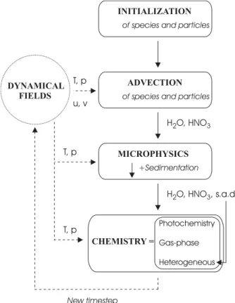
CHEMISTRY = Photochemistry Gas-phase Heterogeneous MICROPHYSICS +Sedimentation H O, HNO , s.a.d.₂ ₃ ADVECTION

of species and particles

H O, HNO₂ ₃

INITIALIZATION

of species and particles

DYNAMICAL FIELDS New timestep T, p u, v T, p T, p

Fig. 1. Schematical presentation of the model, illustrating the cou-pling between the chemical and microphysical modules.

above 21 km, and decreasing below to 1 km at 15 km. At the same time and place, the vertical resolution in potential tem-perature is around 25 K or less below 550 K.

The advection scheme is the flux form semi-Lagrangian transport (FFSLT) algorithm of Lin and Rood (1996), with monotonicity constraints that allow no undershoots or over-shoots in the horizontal directions, and only overover-shoots in the vertical direction. This choice is necessary when the vertical resolution around the tropopause is coarse, as is the case for our model. This is also discussed in detail for the GMI model in Rotman et al. (2001), a model which is comparable to our CTM.

The model uses the short-term forecasts of temperature, horizontal winds and surface pressure issued by the ECMWF operational system (cycle 25r3 and 25r4) with a 6-h time res-olution. Manney et al. (2005) showed that these operational, high-resolution products are well suited for detailed studies of stratospheric polar processes. These ECMWF products are downloaded on a 1◦_×1◦ _{horizontal grid, averaged in a}

mass-conservative way to the model grid and linearly inter-polated in time to the timestep of the CTM. The model inte-gration timestep is 30 min in the low resolution and 15 min in the high resolution case. The vertical velocity is computed by the FFSLT scheme in order to ensure mass conservation with the ECMWF horizontal wind fields, taking into account the time evolution of surface pressure.

Table 1. Particle types described in the model.

Label Description State

STS Sulfate aerosols, which become Liquid supercooled ternary

solutions at low temperatures SAT Sulfuric acid tetrahydrate particles Solid NAT Nitric acid trihydrate particles Solid

ICE Solid ice particles Solid

The chemistry module is built by the Kinetic PreProces-sor (Damian et al., 2002) and is integrated using a third-order Rosenbrock solver (Hairer and Wanner, 1996). The 57 chemical species interact through 143 gas-phase reac-tions, 48 photolysis reactions and 9 heterogeneous reacreac-tions, all listed in the 2003 Jet Propulsion Laboratory compilation (Sander et al., 2003). It is important to note that the chemistry module includes the heterogeneous reactions and that photo-chemical, gas-phase and heterogeneous reactions are solved as one chemical system, in which the surface area densities are provided by the microphysical module.

2.2 The PSC module

The PSC module of DMI (Larsen, 2000) is interactively cou-pled to the 3D-CTM. It describes the evolution in size dis-tribution of the number density and chemical composition of 4 types of particles, listed in Table 1. The size distribution of all particle types is binned on a geometrically increasing volume scale. For the present study the range in particle ra-dius of the bins is 0.002–36 µm and the number of bins is 36. In each bin 4 quantities are stored: the particle num-ber density and the masses per particle of respectively con-densed sulfuric acid, nitric acid and water. Besides the am-bient air temperature and pressure, the PSC module uses the model partial pressures of water vapor and nitric acid as in-puts. These model fields can be changed by the PSC module, as the particles may take up or release water or nitric acid as a consequence of their microphysical evolution. The com-bined surface area density of all particles on a model grid-point is used to calculate the heterogeneous reaction rates which are served as an input to the chemistry module. This illustrates the interactive nature of the coupling between the 3D-CTM and the PSC module, which is schematically pre-sented in Fig. 1. The PSC module has an internal timestep because the microphysical processes may require computa-tional timescales much smaller than the CTM timestep. This internal timestep is made variable to gain computing time and is determined by the smallest timescale involved in the mi-crophysical processes relevant in a specific call to the mod-ule.

(5)

The microphysical processes described by the module are, schematically (see Larsen (2000) for a detailed discussion):

1. homogeneous volume dependent nucleation of ICE out of STS 3–4 K below the ice frost point temperature Tice

(Koop et al., 2000), and homogeneous surface depen-dent nucleation of nitric acid dihydrate (NAD) out of STS (Tabazadeh et al., 2002) above Tice, followed by

(assumed) instantaneous conversion of NAD to NAT. The NAD homogeneous nucleation rates have been re-duced by a factor of 100 following recent studies (Knopf et al., 2002; Voigt et al., 2005; H¨opfner et al., 2006b). 2. nucleation of NAT by vapor deposition of HNO3 and

H2O on pre-activated SAT (Zhang et al., 1996), and

nu-cleation of ICE by vapor deposition of H2O on NAT;

3. dissolution of SAT into STS at low temperatures in the presence of high HNO3 concentrations in the gas

phase, followed by uptake of H2O and HNO3 (Koop

and Carslaw, 1996), and melting of SAT into liquid sul-fate aerosols particles at temperatures above 216 K; 4. condensation and evaporation of HNO3and H2O to and

from STS, NAT and ICE, using the basic vapor diffusion equation and applying a full kinetic approach;

5. mass balance calculations of HNO3and H2O between

gas and condensed phase;

6. sedimentation of particles (Pruppacher and Klett, 1997; Fuchs, 1964). As the size bins are the same everywhere in the model, particles sedimenting from one model layer to the lower one can fall into the appropriate size bin.

To compare with extinction measurements the extinction of the aerosols and PSCs are calculated in the model. This is done using by Mie scattering theory for the spherical par-ticles (STS) and the T-matrix technique (Mishchenko and Travis, 1998) for the non-spherical particles (SAT, NAT, ICE). For the T-matrix calculations a database of expansions of the elements of the scattering matrix in generalised spher-ical functions is used. The recommendations of Mishchenko and Travis (1998) for input parameter settings have been fol-lowed. The database used is for volume-equivalent sizes and an imaginary refractive index of 10−8. The real refractive in-dices used are taken from Krieger et al. (2000) and Scarchilli et al. (2005). For the non-spherical particles an aspect ratio of 1.05 is assumed.

3 Antarctic winter 2003

In this section we present results of simulations for the Antarctic winter of 2003 and comparisons to satellite obser-vations.

3.1 Observational datasets and methodology

For this study of the Antarctic winter 2003 we will com-pare model results to observations from MIPAS/Envisat and POAM III. Here we will shortly present the instruments and their datasets, and the methodology followed for the compar-isons.

MIPAS, or the Michelson Interferometer for Passive At-mospheric Sounding, is a limb-scanning Fourier transform infrared spectrophotometer (Fischer and Oelhaf, 1996; ESA, 2000) onboard Envisat. Envisat’s orbit time is 101 min re-sulting in about 14 orbits per day. There are usually around 1000 MIPAS profiles available per day. Each profile has at most 17 points ranging from about 6 km to about 60 km. The chemical species observed by MIPAS are O3, HNO3, H2O,

NO2, N2O and CH4. We use the offline reprocessed data

version 4.61 for our comparisons.

POAM III is a visible/near infrared solar occultation pho-tometer onboard the French Spot-4 satellite which measures the chemical stratospheric constituents O3, H2O and NO2,

and aerosol extinction in the polar regions (Lucke et al., 1999; Lumpe et al., 2002). Here we use the POAM III ver-sion 4 data. Throughout this text we will denote POAM III by POAM. POAM profiles have a vertical resolution of 1 km. The aerosol extinction profiles reach up to 25 km. The chemical species profiles have a wider altitude range. The POAM line of sight is about 230 km. POAM measures at most 15 profiles per day in each hemisphere, all these pro-files are located at a fixed latitude and with a longitude spac-ing of about 25◦. The latitude at which the profiles are taken varies slowly throughout the year, but remains in the po-lar region. In Antarctic winter periods, the latitude varies smoothly between about 65◦S (winter solstice) and about 87◦S (equinox).

To provide a uniform set-up for the comparison of model results to measured profiles the following methodology will be applied. The model fields have been interpolated in space and time (co-located) to the observed profiles. This inter-polation occurs online, i.e. at the model timestep where a profile is available. This way of working guarantees an op-timal comparison, e.g. in the case of rapidly changing PSC fields. In a practical sense it allows for a considerable lim-itation in model output and hence disk space usage. Then the observed and co-located model profiles, as well as the observational errors, are interpolated to 3 isentropic levels: 425 K, 475 K and 525 K (corresponding to pressure values of approximately 70 hPa, 50 hPa and 40 hPa, and to altitudes of approximately 18 km, 21 km and 23 km). Higher altitude levels were not considered because they are too close to the top POAM retrieval altitude (see also end of Sect. 3.2). Of the interpolated data at these levels the error-weighted aver-age is calculated over 5-day intervals. Since we concentrate on polar winter processes only profiles within the polar vor-tex are taken into account, with the vorvor-tex edge being calcu-lated following the definition of Nash et al. (1996) using the

(6)

dynamical fields interpolated to the high-resolution model grid (see Sect. 2.1). Although we will call the quantities ob-tained in this way error-weighted mean vortex values, it is important to note that they can not be regarded as properly vortex-averaged values, but merely as averages of available values within the vortex.

When POAM samples a water ice cloud, the large solar extinction prevents POAM from performing a measurement. Such points have been removed in the corresponding model data as well before taking the average. Also observations with a negative error have been removed in both the observed and model profiles before taking the average. Negative data, e.g. some POAM extinction measurements, have not been removed because they are meaningful observations as long as their absolute value is smaller than the retrieval random error.

We have chosen to present 5-day averages because they result in much clearer plots than e.g. daily averages. For ex-ample, variability in the POAM extinction data is a convolu-tion of the zonal asymmetry of PSC occurrence and compo-sition, seasonal evolution of PSC forcing, and POAM sam-pling. Here we list a number of issues which could lead to a difference in variability between the model and the observa-tions. POAM has a long line of sight in which various PSC particles could be sampled at various distances (within the same atmospheric layer) rather than that they would all be located at the tangent point, which is where the model cal-culations are done. Furthermore the model produces clouds which are limited by the model’s grid size in coarse-grained conditions and which have uniform properties inside a grid cell. But as an occultation instrument, and even though its retrieval region is comparable to the model’s horizontal grid size, POAM could well sample small localized clouds of high extinction. These will then spuriously be considered as being uniformly distributed over the effective absorption region near the tangent point, leading to an increased ex-tinction value which will be underestimated by the coarse-grained model. Also as an occultation instrument, POAM has a much higher vertical resolution than the model. And finally it is obvious that the coarse-graining of the tempera-ture to the model resolution will have some influence. The aim of the present study is however not to analyze and even-tually correct for this detailed variability (e.g. by introducing sub-grid scale mountain wave parametrizations) but rather to test the overall performance in polar winter processes of the PSC model in the coarse grained model conditions. For this 5-day averages are sufficient. For an further overview of PSC detection by POAM see e.g. Fromm et al. (1999).

In MIPAS observations, cloud-contaminated profiles will lead to uncertainties in the retrieved gas-phase concentra-tions. These profiles can be excluded by examination of the MIPAS cloud index (Spang et al., 2005). However as cloud-contaminated profile retrievals will lead to large er-rors, the error-weighted averaging method proposed here is expected to largely deal with this issue by attributing less

weight to the contaminated profiles. We have verified this us-ing temperature-based profile selection criteria, which indi-cate no qualitative influence in the model-observations com-parisons of profiles with low temperatures, where cloud con-tamination can be expected.

Besides these vortex averaged values, which serve as a quantitative measure for the comparisons, we will also show model fields and superimposed observational data interpo-lated to the 475 K isentropic level for various dates through-out the winter and spring. These 2-D maps add to the quali-tative understanding of the geographical structure of several fields and to the spatial distribution of the observations. 3.2 Initializations

The simulations start on 1 April 2003 and run until 15 De-cember 2003. The model’s chemical fields are initialized from an assimilation of MIPAS/Envisat observations with the 4D-VAR chemical data assimilation system BASCOE (Er-rera and Fonteyn, 2001; Fonteyn et al., 2002, 2004). An ex-ception has been made for polar water vapor, which has been roughly tuned to POAM values. This was done after the ob-servation that there is a substantial systematic difference in polar water vapor as observed by MIPAS and by POAM, with MIPAS water lower by up to about 25% as compared to POAM in the lower stratosphere. MIPAS v4.61 H2O data

are validated so far only outside of the polarhoods (Oelhaf et al., 2004). In the recent validation study by Lumpe et al. (2006) it is found that POAM sunset measurements of wa-ter vapor show a systematic high bias of about 25% in the lower Antarctic stratosphere relative to HALOE, but the bias is considerably lower for the sunrise measurements. HALOE is suggested to have a 5% low bias (Harries et al., 1996; Kley et al., 2000). The latter study also shows that HALOE can show low biases of up to 15–20% with in-situ measure-ments. Because the differences between POAM and MIPAS are comparable to the POAM-HALOE bias, and given the suggested biases in the HALOE data, we assume that tuning the model’s initial state to POAM water vapor is justifiable for the purposes of this paper. The scaling of the initial (as-similated MIPAS) water vapor field is done by deriving scal-ing factors from a 10-day mean POAM water vapor profile in April 2003 and the corresponding mean model profile. Then these scaling factors are applied to the initial model state ev-erywhere poleward of 60◦latitude.

The initial sulfate aerosol size distributions are described by a lognormal function, defined by a median radius rm,

geo-metrical standard deviation σ and number density Nt

(Pin-nick et al., 1976). We estimated these parameters on the condition that the initial lognormal distribution should re-produce the Unified POAM reference background 1 µm ex-tinction monthly means (Fromm et al., 2003). This condi-tion leaves a lot of arbitrariness in fixing the lognormal pa-rameters. We have chosen to take a set of parameters that follows a smooth profile and deviates not too far from the

(7)

0.06 0.1 0.14 15 20 25 r_m [µm] Altitude [km] 1.35 1.45 1.55 15 20 25 σ 9 10 11 12 13 15 20 25 N_t

Fig. 2. Estimated lognormal parameters of the background aerosol size distribution in the Antarctic in April 2003 used to initialize the Antarctic simulations. From left to right: median radius rm,

geometric standard deviation σ and number density Nt.

measurements made by the University of Wyoming’s opti-cal particle counter (Deshler et al., 2003) on balloon flights in the Antarctic over the past decade (T. Deshler, private communication). Our estimated parameters are shown in Fig. 2. Above 23 km, an altitude which corresponds roughly to 525 K, the background aerosol extinction becomes close to zero and the POAM retrieval is dealing with very small signals. Also most of the measurements by T. Deshler do not exceed 23 km. This means that our estimate of the lognormal parameters above 23 km is highly unsure, and this is conse-quently also the case for the background aerosol field used to initialize the model at these altitudes. This is the reason why we restrict the presentation of results to the 525 K level and not higher up.

3.3 Chemical tracers

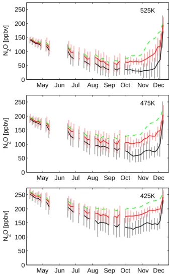
In order to check how well the model calculates the atmo-spheric transport, and more specifically the adiabatic descent of air in the vortex and the dynamical isolation of the vortex, we have compared the evolution of inactive tracer species in the vortex with observational data. A badly performing trans-port would have significant influence on the chemical evolu-tion. Here we compare to the temporal evolution of N2O and

CH4as observed by MIPAS following the methodology

de-scribed in Sect. 3.1. The results are shown in Figs. 3 and 4.

The simulations indicate that the numerical diffusion be-tween the N2O depleted vortex and the surrounding areas is

very large and disturbs the isolation of the vortex consider-ably. This numerical effect is resolution-dependent and is present in all chemical and particle fields with a large gra-dient over the vortex edge (e.g. O3, PSCs). When the

res-olution is too low model grid cells located over the vortex edge sample regions of air both inside and outside the vortex and replace them by a single average value. This increases the values in the region where they are the lowest and vice versa (e.g. for N2O: increase inside the vortex and decrease

outside). The effect decreases with increasing resolution. In

N 2

O [ppbv]

525K

May Jun Jul Aug Sep Oct Nov Dec

0 50 100 150 200 250 N 2 O [ppbv] 475K

0 50 100 150 200 250 N 2 O [ppbv] 425K

0 50 100 150 200 250

Fig. 3. 5-day error-weighted mean vortex N2O mixing ratios of

MIPAS (black) and co-located model results after interpolation of profiles to isentropic levels (red full: high resolution, green dashed: low resolution). The grey-shaded area is the 5-day MIPAS variabil-ity (1 error-weighted standard deviation) while the red-shaded area is the 5-day variability of the high resolution simulation. For all time-series plots in this paper the horizontal axis represents months of 2003. The ticks indicate the first day of each month.

our high resolution simulations the vortex mean N2O values

remain acceptable close to the observations – i.e. well within the MIPAS variability – until the second half of September. By this time most of the polar winter processes are over and the vortex starts to weaken. After this period the model ba-sically overestimates the mixing of polar air when the vortex disappears. It is expected that this could be solved by using a still higher resolution but such a study was beyond the limits of the present computing power.

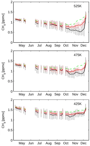
For CH4the model remains much closer to the MIPAS

ob-servations than for N2O (Fig. 4). In the high resolution case

there is nearly a perfect match until October. This differ-ence with the N2O plot is remarkable because of the strong

(8)

Sankey and Shepherd, 2003) from which one would expect both species to follow the same trend under e.g. numerical diffusion. Therefore we think that this difference is likely due to the MIPAS data. Indeed we have verified the N2

O-CH4 correlation in the MIPAS data in the polar vortex (not

shown). We find that the MIPAS data show a considerable amount of scatter, and while on average the correlation fol-lows the fit found in the literature in the beginning of the winter, it deviates from this during mid-winter by overesti-mating CH4. The model preserves the correlations

through-out the simulation period. As there is to our knowledge not yet an published validation of MIPAS data available, it is im-portant to remind that several differences between model and observations presented in this paper could be partially due to inaccuracies in the data.

Of course it can not be ruled out that problems in the verti-cal transport are responsible for part of the deviations in these fields. However the strong resolution dependence seems to indicate that the largest contribution is due to numerical dif-fusion. In this context, we would also like to mention the study of Strahan and Polansky (2006), who showed that a resolution of 2◦×2.5◦is sufficient to isolate the Antarctic po-lar vortex well enough for popo-lar chemistry studies.

3.4 Extinction

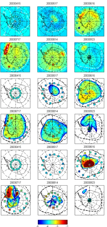
Figure 5 shows the evolution of the high resolution model ex-tinction for STS, NAT and water ice on several dates through-out the winter and spring. Superimposed are the POAM total extinction observations on the same dates. Figure 6 shows the comparison of the calculated extinction at 1020 nm to the extinction as measured by POAM following the methodol-ogy described in Sect. 3.1. The agreement between model and observations is good. The correspondence is excellent on the lowest two levels. The model follows the general trend of the observations with the onset of enhanced extinction in June, the maximum in July and August, and the end of en-hanced extinction in September 2003. The dashed blue line is the evolution of the initial climatological background aerosol extinction, which is treated as a tracer in the model. The im-pact of PSC formation can be seen from the elevation of the extinction above the background level.

A first observation from Fig. 6 is that the horizontal res-olution has not much influence on the calculated extinction. There is only a slight increase in the high resolution results. From this we conclude that the main contribution to the to-tal extinction comes from PSC fields with horizonto-tal scales larger or at least comparable to the grid size of the low reso-lution model grid (see Sect. 2.1).

A general discussion of the differences in variability be-tween POAM and the model was already held in Sect. 3.1. As already mentioned there 5-day averages remove much of the small time-scale and inter-profile variability, and here they indicate that the model produces an acceptable average ex-tinction.

CH

4

[ppmv]

525K

0 0.5 1 1.5 2 CH 4 [ppmv] 475K

0 0.5 1 1.5 2 CH 4 [ppmv] 425K

0 0.5 1 1.5 2

Fig. 4. 5-day error-weighted mean vortex CH4mixing ratios of

MIPAS and co-located model results after interpolation of profiles to isentropic levels. Colors as in Fig. 3.

On the 525 K level the model predicts the onset of en-hanced extinction in the second half of May which is about two weeks too early compared with the observations. From Fig. 6, which also shows the contribution of the various par-ticle types to the total model extinction, it is clear that this problem is not caused by an overestimated early NAT for-mation, but is entirely related to STS. This problem can be caused by the uncertainty in our estimate for the lognormal parameters of the background aerosol distribution at this alti-tude (see Sect. 3.2), or by biases in the temperatures. Gobiet et al. (2005) and H¨opfner et al. (2006b) have reported consid-erable temperature biases in ECMWF analyses in this period (up to 3.5 K). The forecast fields which we use are initialized by these analyses and it is likely that these temperature biases propagate in the forecast fields.

To check this issue we have applied the monthly mean bias corrections which H¨opfner et al. (2006a) derived for the McMurdo station, and which were kindly provided by

(9)

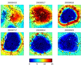
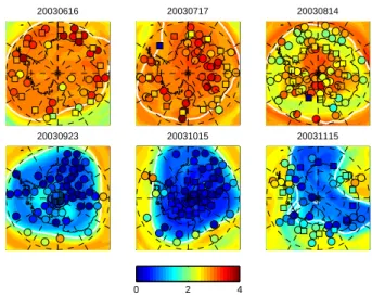
Fig. 5. STS (top), NAT (middle) and ICE (bottom) extinction (km−1, log10 color scale) from the high resolution simulations, interpolated to the 475 K isentropic level, for several dates dur-ing winter and sprdur-ing, always at 12:00 UT. Overimposed are all POAM (squares) total extinction observations of the same day at 475 K±20 K. Transparant squares are locations where no POAM measurement is available, e.g. over the ICE cloud on 17 July. The white (black) dashed line is the polar vortex edge as calculated fol-lowing Nash et al. (1996).

M. H¨opfner, to the entire polar region, and separately we have also applied latitude-resolved monthly mean bias cor-rections derived from CHAMP radio occultation

measure-Extinction [km

−1

] 525K

10−4 10−3 10−2 Extinction [km −1 ] 475K

10−4 10−3 10−2 Extinction [km −1 ] 425K

10−4

10−3

10−2

Fig. 6. 5-day error-weighted mean vortex 1020 nm extinction of POAM (black) and co-located model results (red dashed: low res-olution, red full: high resolution) after interpolation of profiles to isentropic levels. Also shown are the co-located model extinction contributions of the different particle types: STS (green), NAT (ma-genta), and ICE (cyan) for the high resolution simulation. The SAT extinction does not exceed the axis range. The grey-shaded area is the 5-day MIPAS variability (1 error-weighted standard deviation) while the red-shaded area is the 5-day variability of the high reso-lution simulation. Also shown is the model’s background aerosol extinction (dashed blue line).

ments, which were kindly provided by U. Foelsche (Foelsche et al., 2006). Our conclusion from these studies is that for a 3-D Eulerian system such as the one presented here, tem-perature bias corrections need to be more detailed than the monthly averages which are currently available. The latitude resolved data from Foelsche et al. (2006) are already a step forward but both the temporal as well as longitudinal resolu-tion need to be increased for them to have any positive effect on the results. We observe that applying these coarse correc-tions can improve the situation on one location but worsen

(10)

it on another one. This is possibly due to the nature of the biases in the ECMWF fields, and of course deviations may arise because we apply these bias corrections to ECMWF short-term forecast fields while they were derived from the ECMWF analyses.

We want to stress that this problem is intrinsic to our ap-proach. The difference with studies on trajectories is that trajectories are relatively short in time (10 days) and are all independent to some degree (in some approaches the box models on different trajectories can interact). In a full 3-D approach the entire polar region is interacting through the transport, and eventual errors created in the simulations, e.g. too early PSC creation due to a bias in the temperature, can propagate throughout the system, both in space and time. The combination of diffusive transport and complex micro-physics makes the system very sensitive.

Figure 6 illustrates that in the model the main NAT for-mation period occurs at the top levels in the early winter, in the second half of June, while STS is the major PSC type af-ter that period. It is however important to remind here that POAM is prevented from making measurements of optically thick water ice clouds so Fig. 6 does not give an indication of the actual water ice presence. It is clear from Fig. 5 that water ice is the predominant PSC type throughout the winter. On 17 July at ∼315◦longitude there is an example of an obser-vation where POAM was prevented from making an actual measurement. This location coincides perfectly with a large water ice cloud in the model. Where the model finds water ice at the location of the non-excluded POAM observations (see Fig. 6), its contribution is always small compared to the total extinction, which is consistent with the POAM data.

Regarding the first appearance of NAT, H¨opfner et al. (2006b) derived a date of 10 June from MIPAS observations. The model used in that study is basically the same model as the one used here, but in the Lagrangian version, and with the inclusion of mountain wave temperature corrections. The conclusion of H¨opfner et al. (2006b) is that to comply with the MIPAS observations, the NAT freezing mechanism above Tice should not be used in the model. Model studies

in H¨opfner et al. (2006b) with inclusion of this mechanism yield a much earlier date for the first appearance of NAT (23 May).

Although we indeed find that NAT forms already during May, this NAT presence is however very limited. This in-dicates that generally the clouds have a mixed composition, with STS the predominant particle type and only very small amounts of NAT. The NAT extinction becomes comparable to the STS extinction between 6 and 10 June, a few days too early to coincide with the result of H¨opfner et al. (2006b). We have also done simulations with the NAT freezing mech-anism above Ticeturned off, and although the first formation

of NAT in the model is delayed to the beginning of June now, the situation becomes very quickly comparable to the case with this mechanism included, i.e. first appearance of ele-vated NAT extinction between 6 and 10 June. This makes us

20030415 20030517 20030616

20030717 20030814 20030923

0 5 10 15

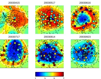
Fig. 7. High resolution model HNO3 field (in ppbv)

interpo-lated to 475 K for several dates during winter and spring, always at 12:00 UT. Superimposed are all MIPAS observations of the same day at 475 K±20 K. The white line is the polar vortex edge as calcu-lated following Nash et al. (1996). The development of denitrifica-tion and the extent of the denitrified region within the polar vortex can be followed.

conclude that the influence of temperature biases and the un-certainties in the background aerosol initialization are domi-nant in this problem, and that no conclusion on the freezing mechanism can be drawn at this stage.

3.5 Denitrification

Figure 7 shows the evolution of the model HNO3 field on

several dates throughout the winter and spring. Superim-posed are MIPAS observations on the same dates. Figure 8 shows the comparison of HNO3between the model and

MI-PAS in the vortex-averaged view as explained earlier. The model overestimates the removal of HNO3everywhere from

mid-June onwards, but this overestimation is much larger on the highest level, while on the lowest two levels the corre-spondence between model and the observations is acceptable (i.e. they remain within each other’s variability). The ex-cessive removal of HNO3during June on the 525 K level is

consistent with an overestimation of the PSC extinction in this period (see Fig. 6) which is likely due to the background aerosol initialization at this level and above (see Sect. 3.2), and also possibly due to the biases in the temperature (see Sect. 3.4).

Figure 7 seems to indicate that the model’s underestima-tion of MIPAS at 475 K originates mainly from contribu-tions in the vortex boundary, where MIPAS sometimes shows some rather elevated values. In the vortex core, which is also the severely HNO3-depleted region of the vortex, the model

values correspond very well with the MIPAS data.

At 525 K, the differences between model and observed HNO3 have a very different cause from mid July onwards.

(11)

HNO

3

[ppbv]

525K

0 5 10 15 HNO 3 [ppbv] 475K

0 5 10 15 HNO 3 [ppbv] 425K

0 5 10 15

Fig. 8. 5-day error-weighted mean vortex HNO₃mixing ratios of MIPAS and co-located model results after interpolation of profiles to isentropic levels. Colors as in Fig. 6.

During the Antarctic winter 2003 high abundances of NOy

of mesospheric/lower thermospheric (MLT) origin were de-posited into the polar stratospheric vortex. Funke et al. (2005) have shown from MIPAS observations that from May to August 2003 high volume mixing ratios of NOx (up to

200 ppbv during the polar night) were transported down-wards from the mesosphere/lower thermosphere into the stratosphere. From this, Stiller et al. (2005) have shown, also from MIPAS observations, that the deposition of MLT NOx caused the formation of a second HNO3 maximum

in the upper stratosphere with volume mixing ratios up to 14 ppbv around 34 km (∼1000 K). This second upper strato-spheric HNO3maximum was transported downwards during

the winter, giving rise to elevated HNO3volume mixing

ra-tios (increases by up to 5 ppbv) around 585 K and below from mid July on. Because the CTM used here does not include a description of the MLT NOxsources, it will not reproduce

the second peak in HNO3. This explains why even from mid

[ppbv] 15 Apr 2003 100 200 300 0 5 10 15 20 25 15 Apr 2003 100 200 300 0 5 10 15 20 25 [ppbv] 16 Jun 2003 100 200 300 0 5 10 15 20 25 16 Jun 2003 100 200 300 0 5 10 15 20 25 [ppbv] 14 Aug 2003 100 200 300 0 5 10 15 20 25 14 Aug 2003 100 200 300 0 5 10 15 20 25 [ppbv] [ppbv] 15 Oct 2003 100 200 300 0 5 10 15 20 25 [ppbv] 15 Oct 2003 [K] 100 200 300 0 5 10 15 20 25 300 400 500 600 700

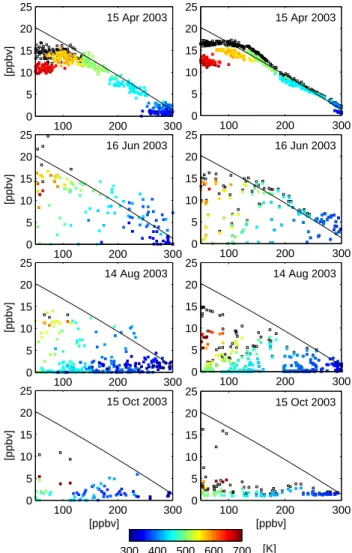
Fig. 9. Scatterplots of HNO₃vs. N₂O for MIPAS data inside the polar vortex (left) and the co-located model data (right) for the high resolution simulation on four dates. The colorshading is the poten-tial temperature. The black line is a fit based on model data of 15 April. In the MIPAS plots the small black squares are HNO3+NO2

and in the model plots the small black squares are the total model NOy.

July onwards HNO3 values observed by MIPAS remain

el-evated over model values throughout the rest of the winter. The differences between model and observations at 525 K can reach up to about 5 ppbv, a value which is comparable to the one mentioned in Stiller et al. (2005).

In the following we will use the correlation between the chemical tracer species N2O and the total amount of reactive

nitrogen NOyto study the denitrification in the model. In a

denoxified and denitrified situation the total NOywill deviate

from this correlation with N2O. This makes this correlation

a useful tool to check the influence of PSCs on the nitrogen budget of the stratosphere. The only NOyspecies measured

in the standard MIPAS product are HNO3and NO2, but the

(12)

In fact as was demonstrated in Kawa et al. (1992) in polar winter conditions NOyconsists almost entirely of HNO3, so

for the observations of MIPAS we can approximate the NOy

-N2O correlation by a correlation between HNO3and N2O. In

Fig. 9 we show scatterplots of HNO3versus N2O of MIPAS

and co-located high resolution model data for four different days throughout the winter and spring: 15 April, 16 June, 14 August, 15 October.

The plot of 15 April illustrates the pre-winter background situation. Only above ∼525 K the deviations between HNO3

and NOy become considerable in the model data. The

ef-fect of ongoing denitrification is clear in the next plots, and a state of nearly total denitrification is visible in the plots for 15 October. Then mixing of extra-vortex air with a higher po-tential temperature starts to occur, and also the repartitioning of nitrogen within the NOyfamily is illustrated in the figure.

From our data on 15 April we derive the following fit for the tracer relation:

NOy=23.5963−0.0661 × N2O−2.6786.10−5× N2O2

(with the NOy and N2O mixing ratios in ppbv). The

lin-ear coefficient of 0.0661 is very comparable to previously re-ported values for the Antarctic, see e.g. Fonteyn and Larsen (1996) and references therein.

The amount of denitrification can be calculated as the dif-ference between NOy under polar winter and early

spring-time conditions and the estimated pre-winter NOy

concen-tration given by this tracer relation. An approximative value for denitrification as observed by MIPAS can then be calcu-lated as the difference between the observed HNO3and NOy

as derived from the observed N2O (Davies et al., 2006).

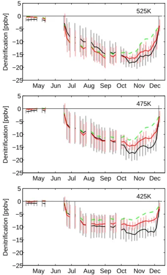
We use this approximative denitrification quantity to com-pare the model to the MIPAS data in a similar set-up as be-fore, see Fig. 10. During April the MIPAS data are slightly negative but this is due to the fact that the curve fit is based on model NOy data, and for MIPAS NOy is only

approxi-mated by HNO3+NO2. The effects of the overestimated

re-moval of HNO3in June and underestimation of HNO3from

mid July onwards, as discussed in the previous section, are visible in the 525 K level. On the lowest two levels the cor-respondence between model and data is exceptionally good. The deviations during late winter and early springtime orig-inate mainly from the problem with N2O (see Fig. 3) due to

numerical diffusion. 3.6 Dehydration

Figure 11 shows the evolution of the model H2O field on

several dates throughout the winter and spring. Superim-posed are MIPAS and POAM observations on the same dates. Figures 12 and 13 show the evolution of water vapor in the vortex-averaged view. The differences in polar water vapor data from both instruments which were already mentioned in Sect. 3.2 are obvious from these plots.

Denitrification [ppbv]

525K

−25 −20 −15 −10 −5 0 5 Denitrification [ppbv] 475K

−25 −20 −15 −10 −5 0 5 Denitrification [ppbv] 425K

−25 −20 −15 −10 −5 0 5

Fig. 10. 5-day error-weighted mean vortex approximative denitri-fication, calculated as the difference between HNO3 and NOy as

calculated from N2O using the fit cited in the text, from MIPAS

ob-servations (black) and co-located model results after interpolation of profiles to isentropic levels. Color legend as in previous figures.

Dehydration occurs because water-rich ice particles sedi-ment when they have grown sufficiently large. The MIPAS data (Fig. 12) show very little variation in the polar vortex water field throughout the winter. The POAM data of Fig. 13 show much more variability and the effect of dehydration is clearly visible. This difference between the two instruments is related to their coverage. While dehydration starts within the polar vortex core, MIPAS samples over the entire vortex and mixes depleted values within the vortex core and still el-evated H2O values in the vortex edge. Because POAM

mea-sures each day at a fixed latitude, which slowly changes in time, the evolution of the data in Fig. 13 is rather a combina-tion of dehydracombina-tion and POAM sampling geometry.

Dehydration starts slowly in June 2003, some weeks later than denitrification which is consistent with earlier studies,

(13)

20030415 20030517 20030616

20030717 20030814 20030923

1 3 5 7

Fig. 11. High resolution model H2O field (in ppmv)

interpo-lated to 475 K for several dates during winter and spring, always at 12:00 UT. Overimposed are all MIPAS (circles) and POAM (squares) observations of the same day at 475 K±20 K. The white line is the polar vortex edge as calculated following Nash et al. (1996).

e.g. Tabazadeh et al. (2000). Then it continues increasingly rapidly throughout July until the beginning of August, when the polar stratospheric water vapor reaches a minimum. At this point about 60% of the initial water vapor amount has been removed. From then on the water vapor starts to in-crease again very slowly with the rise of temperatures, the evaporation of PSCs, the weakening of the vortex and the mixing with extra-vortex air. Substantial dehydration is only present below ∼525 K. All these results are consistent with a recent study of dehydration during the 1998 Antarctic winter using the IMPACT trajectory model (Benson et al., 2006).

At the 475 K level the correspondence between the model and the MIPAS observations is very good during August and September in Fig. 12, while the maps of Fig. 11 show some very elevated values in the MIPAS data. These observations are likely contaminated by clouds because they are excep-tionally high (10 up to 50 ppmv) and have very large errors (over ∼5 ppmv and up to 50% for the highest values). The error-weighting procedure smooths out these outliers and in-dicates that the model corresponds well to the MIPAS data within their error bars.

At the 525 K level the model predicts some dehydration but this is not consistent with the observations. This level is the location of a strong vertical gradient in the water va-por field. The deviations between the model and the POAM observations may well be a consequence of the coarse ver-tical model resolution, which may lead to an overestimated smoothing of the water vapor gradient at this level. But the origin of this problem lies also partially in the initial condi-tions at high altitudes. Although the initial model water va-por field was tuned to the POAM water vava-por (see Sect. 3.2),

H 2

O [ppmv]

525K

0 2 4 6 8 10 H 2 O [ppmv] 475K

0 2 4 6 8 10 H 2 O [ppmv] 425K

0 2 4 6 8 10

Fig. 12. 5-day error-weighted mean vortex H2O mixing ratios of

MIPAS (black) and co-located model results after interpolation of profiles to isentropic levels. Color legend as in previous figures.

this tuning was done rather conservatively at altitudes above 25 km. Differences of 1.5 ppmv or more exist in the initial (tuned) model field and the POAM data at altitudes between 35 km and 40 km. Due to downward motion within the vor-tex, these differences have descended to the 525 K level by August.

It is likely that the deviations in water vapor, especially during August, are partly responsible for the underestimation in the model extinction during this period (Fig. 6).

3.7 Ozone depletion

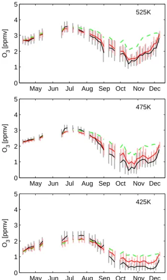
Finally we have compared the evolution of model polar ozone to observations of MIPAS and POAM. The results are shown in Figs. 14, 15 and 16. The model reproduces the ob-servations very well. When in the springtime the polar vortex becomes depleted with ozone due to chemical destruction, and the surrounding area, in full sunlight and in absence of

(14)

H 2

O [ppmv]

525K

0 2 4 6 8 10 H 2 O [ppmv] 475K

0 2 4 6 8 10 H 2 O [ppmv] 425K

0 2 4 6 8 10

Fig. 13. 5-day error-weighted mean vortex H2O mixing ratios of

POAM (black) and co-located model results after interpolation of profiles to isentropic levels. Color legend as in previous figures.

active chlorine, becomes enhanced with ozone, the numeri-cal diffusion will play an important role. During the maxi-mum of the ozone hole conditions (second half of September and throughout October) the low resolution simulation stays about 0.5-1 ppmv above the observations. The high resolu-tion simularesolu-tion improves these deviaresolu-tions by ∼50% at the lowest levels, and it nearly matches the MIPAS data at the 525 K level.

It is obvious from the plots that horizontal resolution is a major factor in an accurate simulation of the ozone deple-tion of the vortex. This indicates that the PSC modelling and the related chemical processes are performing well. Good agreement is most difficult to reach at the lowest levels be-cause the observed ozone concentrations on those levels are nearly zero, making the simulations very sensitive to numer-ical diffusion. It concerns here not only a problem due to the numerical diffusion of ozone alone across the vortex edge but

20030616 20030717 20030814

20030923 20031015 20031115

0 2 4

Fig. 14. High resolution model O3 field (in ppmv)

interpo-lated to 475 K for several dates during winter and spring, always at 12:00 UT. Overimposed are all MIPAS (circles) and POAM (squares) observations of the same day at 475 K±20 K. The white line is the polar vortex edge as calculated following Nash et al. (1996).

an accumulated effect of the numerical diffusion in various fields with strong cross-vortex edge gradients such as HNO3

(Fig. 8, and the resulting denitrification, Fig. 10), the PSCs, and active chlorine.

Our conclusion is consistent with the study of Hoppel et al. (2005), which demonstrated that accurate dynamics is a key ingredient for correctly modeling the spatial distribution of Antarctic ozone loss.

4 Discussion

4.1 Conditions of model coupling

Addressing the mathematical and numerical conditions for the coupling of the two models, i.e. the global CTM and the microphysical model, is a nontrivial issue. It is obvious that we have not entered yet a rigorous discussion of this prob-lem, but hope to have reached some empirical insight with the case study presented in the previous section. Moreover we have tested the robustness of the coupling with some ad-ditional sensitivity tests which have not yet been presented above. We think that the main numerical control parame-ters in the coupling of the models are threefold: the horizon-tal and temporal resolution, the size bin resolution, and the transport scheme.

For what concerns the horizontal resolution, it is some-what surprising that increasing the resolution by 4 has only a small influence on the calculated extinction (Fig. 6). We can conclude that even in the lower resolution case, the polar grid cells are already smaller or at least comparable in size to the typical scale of PSCs. Increasing the horizontal resolution

(15)

O 3

[ppmv]

525K

0 1 2 3 4 5 O 3 [ppmv] 475K

0 1 2 3 4 5 O 3 [ppmv] 425K

0 1 2 3 4 5

Fig. 15. 5-day error-weighted mean vortex O3mixing ratios of

MIPAS (black) and co-located model results after interpolation of profiles to isentropic levels. Color legend as in previous figures.

by 4 may lead to local temperature refinements, but will not lead to major changes in the PSC field. Therefore we could conclude empirically that a resolution of 3.75◦ by 5◦ is in principle sufficient to study at least synoptic-scale PSCs in the Antarctic. However as stated before the main benefit of the resolution increment lies in the improvement in numeri-cal diffusion.

We have increased the number of bins up to 96, but no sig-nificant improvements have been found, indicating that 36 size bins is a sufficient resolution for the studies presented here. Because even 36 size bins is computationally quite de-manding (adding 4 types × 36 bins × 4 quantities = 576 extra tracers to the model) we also have checked the influence of lowering the number of size bins. In simulations using 12 bins the accuracy of the results decreased. For all fields still a comparable behaviour was found as in the 36 bin case, but most results were worse compared to the 36 bin case by some

O 3

[ppmv]

525K

0 1 2 3 4 5 O 3 [ppmv] 475K

0 1 2 3 4 5 O 3 [ppmv] 425K

0 1 2 3 4 5

Fig. 16. 5-day error-weighted mean vortex O3mixing ratios of

POAM (black) and co-located model results after interpolation of profiles to isentropic levels. Color legend as in previous figures.

percents. This can indicate that some detailed microphysical behavior can not well be simulated when the number of size bins becomes too small.

Perhaps the main problem with our present approach lies in the fact that clouds are not treated as entities but that all size bins are treated independently under transport. This leads to numerical diffusion which will have an impact on the microphysical evolution. Indeed particles in a specific size bin which after advection end up divided over several grid cells will undergo a different microphysical evolution than if they all would have been transported into one grid cell.

This illustrates again the differences of the present ap-proach with those using Lagrangian models, an issue which had already been addressed in the introduction. Such mod-els are not confronted with the problems regarding diffusive transport. However the only trajectory-based models with a

(16)

complete description of sedimentation, i.e. DLAPSE and the recent version of CLaMS, are at present only designed for the description of NAT particles.

4.2 Model sensitivities

Besides the sensitivity studies mentioned in the previous sec-tion, several other factors play a role in the performance of the model. E.g. the influence of the choice of parameters for the lognormal background aerosol distribution (see Fig. 2) has also been studied to some extent. The main conclusion of this study is that when the initial total number density of aerosols is too small, these few particles grow too large in size since they have all nitric acid at their disposal. The sedimentation occurs too fast and the polar stratosphere be-comes nearly depleted with aerosols by mid-winter. Then from mid-winter onwards the PSC extinction is severely un-derestimated and as a consequence the model fails to repro-duce the springtime ozone depletion.

From the CTM point of view, a major influence on the PSC formation is the water vapor in the model. The issue of initial water vapor has been discussed before (Sect. 3.2). Initializing the model with the MIPAS water vapor which is about 20% or more lower reduces the calculated extinction by a comparable amount (not shown). As mentioned already in Sect. 3.6 also biases in the water vapor initialization at high altitudes have an impact in the later stages of the winter because of the adiabatic descent of air inside the vortex.

And finally there is the impact of the biases in the ECMWF temperatures during this Antarctic winter. In this respect we can mention the study of Benson et al. (2006) again which showed that temperature biases are the main sensitiv-ity parameter in modelling Antarctic extinction and dehydra-tion. Nevertheless the model performed acceptably well on an overall scale although uncorrected temperature data were used. In detailed issues, such as the formation of the first PSCs in the early stages of the winter, the temperature bi-ases undoubtedly have an important impact, see Sect. 3.4. As mentioned in that section we have applied several coarse temperature bias-correction schemes, but these did not im-prove the results. Much more detailed correction schemes, both in space and time, are needed for them to have any pos-itive influence on the model results.

4.3 NAT freezing mechanism

The question of a freezing mechanism for NAT above Tice

has been addressed numerous times already in the literature. For a previous discussion see e.g. Svendsen et al. (2004). It is our opinion that currently we are not able to assess details of the NAT nucleation. There is observational evidence in the Arctic that NAT can form at temperatures above Tice(Larsen

et al., 2004; Voigt et al., 2005). However, we cannot say if this occurs through heterogeneous nucleation, through NAD and (rapid) conversion to NAT, or directly to NAT. We use

the parametrisation of Tabazadeh et al. (2002) with the ap-plied corrections because this is presently the only available parametrisation, based on laboratory measurements. The fact that MIPAS does not see NAD, as found by H¨opfner et al. (2006b), could be due either to the absence of NAD forma-tion, or to a very fast transition from NAD to NAT – too quick to be detected.

Finally it is interesting to mention the actual freezing rates we have found in the simulations, using the rates of Tabazadeh et al. (2002) reduced by 100. The highest values we obtain are of order ∼10 m−2s−1× surface area. These are somewhat smaller but not too different from the ones measured by Larsen et al. (2004) and Voigt et al. (2005), i.e. ∼10−6cm−3h−1for NAT particles of a few µm radius.

5 Summary and conclusions

We have shown that the combined approach of a detailed microphysical model running online in the coarse-grained conditions of a global CTM with full chemistry gives excel-lent results for polar winter processes. By simultaneously comparing PSC extinction, denitrification, dehydration and ozone depletion to a diverse set of observational data we have shown that this approach leads to acceptable and consistent results, leaving mainly the horizontal model resolution, the background aerosol initialization, and the temperature accu-racy as key ingredients for further improvements in ozone depletion.

As explained before the resolution of 1.875◦_×2.5◦_{is our}

current computational limit because of the demanding micro-physical module with 36 size bins. Although in the past de-tailed microphysics in a 3D-CTM has not been considered at-tractive because of the considerable computational demands, we have illustrated that such an approach is feasible. On a recent 32 CPU machine the low resolution runs take about 10 min walltime per simulated day, while the high resolution runs take about 50 min walltime per simulated day, which means simulating a month in the high resolution case takes about one day walltime.

The present approach is suited to the study of the four main PSC particle types: STS, SAT, NAT and water ice particles. It includes a full description of size distribution and composi-tion as well as transport of liquid binary and ternary aerosols and the solid PSC particles, and treats sedimentation in a cor-rect and straightforward way. The integrated approach allows for a full online coupling between the PSC microphysics and the stratospheric chemistry. Finally, the detailed microphys-ical information of the model allows for the calculation of optical properties and in this way model results can be com-pared simultaneously to optical and chemical observational data.

Acknowledgements. The authors wish to thank the Belgian Federal Science Policy for providing the funding in the framework of the Belgian Prodex Program. N. Larsen is supported by the EU project

(17)

SCOUT-O3. The authors greatly acknowledge the European Centre for Medium-Range Weather Forecasts for providing the dynamical forecasts. We thank U. Foelsche and M. H¨opfner for providing temperature bias corrections, and G. Stiller for commenting on the influence of MLT NOxon our results.

Edited by: U. P¨oschl

References

Benson, C. M., Drdla, K., Nedoluha, G. E., Shettle, E. P., Hop-pel, K. W., and Bevilacqua, R. M.: Microphysical modeling of southern polar dehydration during the 1998 winter and compari-son with POAM III observations, J. Geophys. Res., 111, D07201, doi:10.1029/2005JD006506, 2006.

Carslaw, K. S., Kettleborough, J., Northway, M. J., Davies, S., Gao, R.-S., Fahey, D. W., Baumgardner, D. G., Chipperfield, M. P., and Kleinbohl, A.: A Vortex-Scale Simulation of the Growth and Sedimentation of Large Nitric Acid Hydrate Particles, J. Geo-phys. Res., 107, 8300, doi:10.1029/2001JD000467, 2002. Chipperfield, M. P.: Multiannual Simulations with a

Three-Dimensional Chemical Transport Model, J. Geophys. Res., 104, 1781–1805, 1999.

Damian, V., Sandu, A., Damian, M., Potra, F., and Carmichael, G.: The Kinetic PreProcessor KPP – A Software Environment for Solving Chemical Kinetics, Computers and Chemical Engineer-ing, 26, 1567–1579, 2002.

Davies, S., Mann, G. W., Carslaw, K. S., Chipperfield, M. P., Reme-dios, J. J., Allen, G., Waterfall, A. M., Spang, R., and Toon, G. C.: Testing our understanding of Arctic denitrification us-ing MIPAS-E satellite measurements in winter 2002/3, Atmos. Chem. Phys., 6, 3149–3161, 2006,

http://www.atmos-chem-phys.net/6/3149/2006/.

Dessler, A. E.: The chemistry and physics of stratospheric ozone, Academic Press, London, San Diego, 214 pp, 2000.

Deshler, T., Hervig, M. E., Hofmann, D. J., Rosen, J. M., and Liley, J. B.: Thirty years of in situ stratospheric aerosol size distribution measurements from Laramie, Wyoming (41◦N), us-ing balloon-borne instruments, J. Geophys. Res., 108(D5), 4167, doi:10.1029/2002JD002514, 2003.

Drdla, K.: Applications of a Model of Polar Stratospheric Clouds and Heterogeneous Chemistry, Ph.D. thesis, Univ. of California, Los Angeles, Los Angeles, 1996.

Drdla, K., Schoeberl, M. R., and Browell, E. V.: Microphysical modeling of the 1999–2000 Arctic winter, 1, Polar stratospheric clouds, denitrification, and dehydration, J. Geophys. Res., 107, 8312, doi:10.1029/2001JD000782, 2003.

Errera, Q. and Fonteyn, D.: Four-dimensional variational chemi-cal assimilation of CRISTA stratospheric measurements, J. Geo-phys. Res., 106, 12 253–12 265, 2001.

European Space Agency (2000): Envisat: MIPAS, An instrument for atmospheric chemistry and climate research, ESA SP-1229, Noordwijk, Netherlands, 2000.

Fahey, D. W., Gao, R. S., Carslaw, K. S., Kettleborough, J., Popp, P. J., Northway, M. J., Holecek, J. C., Ciciora, S. C., McLaugh-lin, R. J., Thompson, T. L., Winkler, R. H., Baumgardner, D. G., Gandrud, B., Wennberg, P. O., Dhaniyala, S., McKinney, K., Pe-ter, Th., Salawitch, R. J., Bui, T. P., Elkins, J. W., WebsPe-ter, C. R., Atlas, E. L., Jost, H., Wilson, J. C., Herman, R. L., Kleinb¨ohl,

A., and von K¨onig, M.: The detection of large HNO3-containing particles in the winter Arctic stratosphere, Science, 291, 1026– 1031, 2001.

Fischer, H. and Oelhaf, H.: Remote sensing of vertical profiles of atmospheric trace constituents with MIPAS limb emission spec-trometers, Appl. Opt., 35(16), 2787–2796, 1996.

Foelsche, U., Borsche, M., Steiner, A. K., Pirscher, B., Lackner, B. C., Gobiet, A., and Kirchengast, G.: CHAMP Radio Occul-tation Based Climatologies for Global Monitoring of Climate Change, WegCenter Rep. for FFG-ALR No. 3/2006, 52p., We-gener Center, Univ. of Graz, Austria, http://www.uni-graz.at/ igam-arsclisys/ – Publications, 2006.

Fonteyn, D. and Larsen, N.: Detailed PSC formation in a two-dimensional chemical transport model of the stratosphere, Ann. Geophys., 14, 315–328, 1996,

http://www.ann-geophys.net/14/315/1996/.

Fonteyn, D., Bonjean, S., Chabrillat, S., Daerden, F., and Errera, Q.: 4D-VAR chemical data assimilation of ENVISAT chemical products (BASCOE): validation support issues, in: Proceedings of the “ENVISAT validation workshop” held at ESRIN, Frascati, Italy, 9–13 December 2002.

Fonteyn, D., Lahoz, W., Geer, A., Dethof, A., Wargan, K., Stajner, L., Pawson, S., Rood, R. B., Bonjean, S., Chabrillat, S., Daerden, F., and Errera, Q.: MIPAS Ozone Assimilation, Proceedings of the Second Workshop on the Atmospheric Chemistry Validation of ENVISAT (ACVE-2), 3-7 May 2004, ESA-ESRIN, Frascati, Italy (ESA SP-562), edited by: Danesy, D., p. 19.1–19.6, pub-lished on CDROM, 2004.

Fromm, M., Bevilacqua, R. M., Hornstein, J., Shettle, E., Hoppel, K., and Lumpe, J. D.: An analysis of Polar Ozone and Aerosol Measurement (POAM) II Arctic polar stratospheric cloud obser-vations, 1993–1996, J. Geophys. Res., 104(D20), 24 341–24 357, 1999.

Fromm, M., Alfred, J., and Pitts, M.: A unified, long-term, high-latitude stratospheric aerosol and cloud database using SAM II, SAGE II, and POAM II/III data: Algorithm description, database definition, and climatology, J. Geophys. Res., 108(D12), 4366, doi:10.1029/2002JD002772, 2003.

Fuchs, N. A.: The mechanics of aerosols, Pergamon Press, New York, 408 pp, 1964.

Funke, B., Lopez-Puertas, M., Gil-Lopez, S., von Clarmann, T., Stiller, G. P., Fischer, H., and Kellmann, S.: Down-ward transport of upper atmospheric NOx into the polar strato-sphere and lower mesostrato-sphere during the Antarctic winter 2003 and Arctic winter 2002/2003, J. Geophys. Res., 110, D24308, doi:10.1029/2005JD006463, 2005.

Gobiet, A., Foelsche, U., Steiner, A. K., Borsche, M., Kirchengast, G., and Wickert, J.: Climatological validation of stratospheric temperatures in ECMWF operational analyses with CHAMP radio occultation data, Geophys. Res. Lett., 32, L12806, doi:10.1029/2005GL022617, 2005.

Grooß, J.-U., Günther, G., Konopka, P., Müller, R., McKenna, D. S., Stroh, F., Vogel, B., Engel, A., Müller, M., Hoppel, K., Bevi-acqua, R., Richard, E., Webster, C. R., Elkins, J. W., Hurst, D. F., Romashkin, P. A., and Baumgardner, D. G.: Simulation of ozone depletion in spring 2000 with the Chemical Lagrangian Model of the Stratosphere (CLaMS), J. Geophys. Res., 107(D20), 8295, 10.1029/2001JD000456, 2002.