Anisotropy development during HDPE necking studied at the microscale with in situ continuous 1D SAXS scans

HAL Id: hal-01652805

https://hal.archives-ouvertes.fr/hal-01652805

Submitted on 30 Nov 2017

HAL is a multi-disciplinary open access

archive for the deposit and dissemination of sci-entific research documents, whether they are pub-lished or not. The documents may come from teaching and research institutions in France or abroad, or from public or private research centers.

L’archive ouverte pluridisciplinaire HAL, est destinée au dépôt et à la diffusion de documents scientifiques de niveau recherche, publiés ou non, émanant des établissements d’enseignement et de recherche français ou étrangers, des laboratoires publics ou privés.

Anisotropy development during HDPE necking studied

at the microscale with in situ continuous 1D SAXS scans

Laurent Farge, Julien Boisse, Isabelle Bihannic, Ana Diaz, Stéphane André

To cite this version:

Laurent Farge, Julien Boisse, Isabelle Bihannic, Ana Diaz, Stéphane André. Anisotropy development during HDPE necking studied at the microscale with in situ continuous 1D SAXS scans. Journal of Polymer Science Part B: Polymer Physics, Wiley, 2017, 56 (2), pp.170-181. �10.1002/polb.24527�. �hal-01652805�

Anisotropy development during necking of HDPE studied at the

microscale with in situ continuous 1D SAXS scans.

FARGE Laurent

1

_,

_{BOISSE Julien}

1

_{, BIHANNIC Isabelle}

2

_,

DIAZ Ana

3

_{, ANDRE Stéphane}

1*

1_{LEMTA – CNRS – University of Lorraine, 2 avenue de la forêt de Haye, TSA 60604,}

54518 VANDOEUVRE-LES-NANCY, FRANCE

2 _{LIEC – CNRS – University of Lorraine, 15 Avenue du Charmois}

54500 VANDOEUVRE-LES-NANCY, France

3 _{Paul Scherrer Institut, CH-5232 Villigen PSI, Switzerland}

* Corresponding author

[email protected]

Abstract:

Quantitative information about microstructural reorganizations which occur during mechanical solicitation is important to increase our knowledge on the rheology of semi-crystalline polymers. This point is investigated here on High Density Polyethylene through the measurement of an anisotropy index calculated from small-angle X-ray scattering (SAXS) patterns. These were obtained in situ on a coherent synchrotron beamline with a very fast scanning of the specimen under tensile test. This allows the anisotropy development of many material points which undergo different deformation paths to be followed, thanks to necking development and propagation. With this field information, the microstructural anisotropy observable is shown to have a given value at a given true strain, meaning that strain pilots the bulk topology. Results apparently departing from that premise are shown indeed to be an experimental artifact: true strains are measured on the specimen surface, necking introduces strain heterogeneities in thickness, and the SAXS technique probes the full volume producing averaging.

Keywords: synchrotron, small angle X-ray scattering experiments, microstructural

anisotropy, plasticity, kinematics of necking, semi-crystalline polymers, High Density Polyethylene.

Pre-refereeing

version

published

in JPSB

1. INTRODUCTION

Predicting the mechanical behavior of complex materials like semi-crystalline Polymers (SCP) is still challenging especially when dealing with high deformation states beyond the development of plastic instabilities. Numerous recent industrial concerns and trends such as environmental issues show an interest in a massive use of thermoplastics in all type of composite materials as well as for bio-based thermoplastics. Regarding the latter, the chemical modifications needed, if only to achieve the same mechanical properties as petroleum-based thermoplastics, are currently determined by trial and error. An extended understanding of the basic strain-driven phenomena proceeding in a semi-crystalline structure is probably the key for more guidance in the development of such materials with more or less targeted properties.

In brief, the challenge now is the elucidation of the sequence of micromechanisms of deformation which range from an initial architecture of spherulitic packing to a fibrillar microstructure [Galeski, 2003]. Spherulite is a complex heterogeneous structure made of crystal lamellae and amorphous domains. All scales are concerned, which raises experimental complexities due to both the limited range of scale probed by the various available techniques and the interpretation and establishment of quantitative observables from the measured data. Looking at the researchers' practices in material sciences, a review of the literature shows immediately that the vast variety of studies (different selected aims and materials) form an additional obstacle to obtain a unified and complete view of the subject.

Among contemporary studies on SCPs, especially on polyethylene, which can introduce the topic, we favor the most recent ones or those where small angle X-ray scattering (SAXS) experiments are conducted under in situ conditions using a synchrotron X-ray beam. One can cite first the works of Butler and coll. [Butler et al., 1995] on Polyethylene specimens with thicknesses ranging from 0.9 to 1.9 mm subjected to tensile loading. Their studies produced a wide experimental collection of WAXS/SAXS patterns from which they established (and/or confirmed) the sequence of micro-mechanisms that the material underwent in the q-range [0.05-0.6] nm-1 where q is the modulus of the scattering vector. They essentially showed that the onset of a phase transformation in the crystalline phase

Pre-refereeing

version

published

in JPSB

(WAXS analysis) occurred simultaneously with the onset of cavitation (SAXS analysis), that a loss of isotropy accompanied deformation, and that inter-lamellar shear occurred in the amorphous phase. Next, studies [Butler et al., 1997a, 1997b] brought additional insights related to these experimental facts and specimens thermal history as well as their material macromolecular parameters. Schneider and al. [2006] used such experiments to study the nanocavitation phenomenon occurring during the necking of HDPE (High Density Polyethylene) under tensile testing up to true strains of 2. They proceeded more or less in the same way as we did in the present work, but only monitored what happened to the central point of their specimen and for a narrower q-range [0.08-0.8 nm-1]. They focused mainly on the qualitative analysis of intensity profiles obtained both on WAXS and SAXS images, to discuss the synopsis of nanovoid deformation supported by their observations. While the authors commented on the anisotropy effect observed on SAXS patterns, especially the favored transversal orientation in the first plastic regime, they did not set up a quantitative observable from the data. Humbert et al. [2010] carried out the same study on HDPE for different specimens having controlled different microstructures. SAXS measurements were also performed in situ thanks to a synchrotron X-ray source for a wider q-range of [0.05-0.95] nm-1. The study was restricted to true strains below 0.6. SAXS patterns were quantitatively analyzed through the form factor of scatterers assumed to have a cylindrical geometry. The scatterers are clearly considered as one-body voids due to cavitation, of size limited to a few tens of nm. Although very qualitative, bringing this phenomenon together with whitening of the specimen is not strictly possible. Unfortunately neither intensity profiles nor information about the inverse process leading to estimate the microstructural parameters from them were provided. Focusing only on SAXS experimental investigations, most studies on SCPs were interested in following the development of the nanocavitation phenomenon [Rozanski et al., 2011, Schneider K., 2010]. The study of the effect of temperature, or of an annealing treatment of the microstructure under stretching, is another example of specific studies aimed in the present case to understand the close relation between the lamellar stack organization evolution and stress or temperature [Jiang et al., 2007, Xiong, 2014]. In a recent paper of Zhao [Zhao et al., 2016], experimental SAXS investigation is used to understand more clearly the fibrillar state, at high true strains (about 1.3) with respect to the hardening or elasticity reinforcement.

Pre-refereeing

version

published

in JPSB

Concerning our motivations, it is worthy of mention that our main initial interest was to capture the kinetics of various individual phenomena during the deformation process. The final motivation was to identify any recursive or fractal behavior of microstructural events (for a homogeneizable bulk microstructure). On the one hand, behavior models that are based on a recursive or fractal spectrum of relaxation times were proved pertinent to describe the kinetics of micromechanisms of deformation through a modal approach [Andre et al., 2003, Blaise et al., 2016]. On the other hand, physical evidence of a kind of similarity in the scale-spreading sequence of micromechanisms of deformation have been obtained that are quasi inexistent in polymer science [Farge et al, 2013]. They were gathered by monitoring an observable quantitative and measuring the anisotropy which develops in bulk at all scales.

In this paper, we focus on SAXS experiments for an [0.01-1] nm-1 q-range which means that the range of scale lengths investigated runs approximately from 1nm to some 100 nm. Quantitative post-treatments of SAXS data collected on an extensively studied HDPE allow an anisotropy index from the recorded 2D scattering patterns to be calculated. Based on this observable, we now address the following question: is it possible to consider that the topological characteristics of a given deformed microstructure are ruled solely by the current true strain (independently of the strain or load path)? The answer will be obtained by investigating what happens to different material points subjected to a different strain path in a tensile test. This difference in strain path occurs automatically within the plastic instability that develops once the yield stress is reached and necking occurs.

In Section 2, the material, experimental technique, and methodology of post-treatment will be presented. SAXS patterns were recorded continuously and in-situ with high-speed scanning at very high spatial resolution. This allows for 1-D cartography of the specimen during tension. Precise calibration of the deformation kinematic was obtained through Digital Image stereo-Correlation (DIC) measurements. The relationships between time, material coordinate, Eulerian position and local true strain will be clearly given through calibration curves. They ensure the quality of the analysis.

In section 3, the results are given, showing the evolution of the anisotropy of the microstructure for different material points and different levels of strain. The intrinsic

Pre-refereeing

version

published

in JPSB

character of this variable (absolutely determined by the microstructure topological organization) will be checked against results obtained on two different specimens of different thicknesses. These results will be commented within the frame of our current knowledge on the subject. Thanks to this methodology, the intensity profile sequences will be given as a function of the strain in both the tensile and transverse directions with extremely high statistics, as a result of the original scanning methodology used in this study.

In section 4, a qualitative 3-D analysis of the mechanical behavior of the necking phenomenon is produced thanks to Finite Element (FE) simulations. Although not perfect, it quantifies the slight heterogeneity in longitudinal strain that exists along the beam path. In view of the average bulk probing that results from X-ray scattering, it explains naturally the apparent small departure of our anisotropy measurements from being set to a constant value for a given strain, when this latter is considered as the surface strain for evident experimental reasons. This analysis justifies our conclusive statement.

Pre-refereeing

version

published

in JPSB

2. MATERIAL AND METHODS Material

The material under investigation is a HDPE produced by Röchling Engineering Plastics KG ("Natural 500" grade). Considered as a "model" SCP, this material has been studied at all scales for more than 15 years. The material is supplied as sheets obtained from an industrial scale extrusion process and specimens were all cut with the extrusion direction corresponding to the tensile test axis. Bone-shaped specimens (see Fig. 1, Blaise et al., 2011) were designed to have a small central cubic part - the Representative Volume Element (RVE) - in order to control the localization and development of the plastic instability exactly in the middle of the specimens. The loading path that the specimens underwent was pure tension but up to very large true strains (a Hencky strain of nearly 2 was reached in RVE, the most deformed central part). Two geometries of specimen are considered here with a central cubic part of either 3mm or 6mm gauge (hereinafter referred to as HDPE3 and HDPE6 respectively). As a result of these two different gauge sizes, the shapes of the specimen (curvature radii) differ slightly. This is interesting for the study as it allows (i) to subject the specimen material points to different loading and strain paths and (ii) to check the consistency of the SAXS results for two different thicknesses of material crossed by the beam.

The main characteristics of this polymer are: molecular weight of 500,000 g/mol , density of 0.935 g/cm3, crystallinity index of 67% (DSC and WAXS assessment), microstructural dimensions of 26.8 nm for the long period of the stack, 18.5 nm for the crystalline phase thickness and 8.2 nm for the amorphous layer thickness (SAXS characterization). A census of our main studies where complementary information can be found in the various characterizations made at all scales, from the Å to the mm, can be read in [Farge et al., 2013 and 2015].

SAXS measurements at PSI cSAXS beamline and experimental conditions.

SAXS data were acquired at the coherent small angle X-ray scattering beamline (cSAXS) at the Swiss Light source (SLS) in the Paul Scherrer Institut in Villingen, Switzerland, for a photon light energy of 11.2 keV corresponding to a wavelength of 1.106Å. The

Pre-refereeing

version

published

in JPSB

approximate beam size at the specimen was 150x200m. SAXS patterns were recorded with a 2M-Pilatus detector [Heinrich et al., 2009] with 1475 × 1679 pixels (horizontal  vertical) of 172 × 172 μm2 resulting in an active area of 253.7 × 288.8 mm. It consists of 3 × 8 detector modules each of 487 × 195 pixels, separated by the equivalent of 7 pixels horizontally and 17 pixels vertically. The area between the modules is not sensitive to X-rays and is not considered for quantitative analyses. Standard calibration procedures were performed using AgBeOH, Glassy Carbon, Si and LaB6 reference materials. With AgBeOH, the detector-specimen distance has been determined to be 7168 mm, which gives a q-range of [0.017-1] nm-1, corresponding to length scales ranging approximately from 10 to 350 nm. The SLS synchrotron has operated in a top-up mode for many years with an injection efficiency from the booster to the storage ring that is close to 100%. This ensured good flux stability at the exit beam pipe and combined to the high performance of the Pilatus detector, signals are of very high quality.

Figure 1: View of the experimental setup at the cSAXS beamline

Experiments were performed using a Kammrath & Weiss mini-machine to perform the tensile tests in situ under the beam. The machine subjects specimens to drawings at constant displacement rates. The central point remains fixed as the two grips move apart from each other thanks to two contra-rotative screws. The machine was mounted on two linear translation stages (see Fig. 1) allowing for in-plane displacement at a maximum velocity of 10mm/s to produce 1D or 2D scans.

Concerning the scanning parameters, the integration time of the detector was 33 ms, and the read out time 3ms, which made a spatial resolution of 360m at the 10mm/s

Pre-refereeing

version

published

in JPSB

displacement rate used in the scanning process. At the same time, the tensile machine proceeded with a displacement rate of 20 m/s, corresponding to a negligible displacement of the material points on the specimen during a full scan along the specimen central axis. The scan's initial and final position were modified automatically according to the length increase of the specimen gauge. This meant that the number of measurement points where intensity patterns were recorded increased with the experiment time. The dots of Fig. 2 following a repeated N-shaped path along the horizontal time axis gave all SAXS pattern positions in the fixed laboratory reference frame (Eulerian positions). As an example, if at a given time of the experiment a 20 mm length had to be scanned, it would be done in 2 seconds. During this time the grips of the tensile machine only moved apart from a 40m distance, while more than 50 SAXS images were taken. The acquisition time of each SAXS pattern allowed the corresponding spatial position on the specimen to be given, thanks to a calibration procedure which is presented next.

Figure 2: Correspondences between SAXS pattern positions and acquisition times and DIC data as a result of the calibration procedure – Gray dots correspond to the positions where

SAXS images were recorded.

Pre-refereeing

version

published

in JPSB

At this stage, one must bear in mind that during a single test, approximately 208 scans are performed, with about 17000 SAXS patterns being recorded. This suggests dedicated data processing to deal with this huge amount of data.

Conversion between Eulerian and Lagrangian configurations

To investigate microstructural mechanisms of deformation, it is important to be able to connect observed quantities to the exact material point or local volume where they are measured. We speak of a material "grain" when the material point of view is associated with the idea that measurements are taken on a small representative elementary volume centered on a given material point. Because in the present case the tensile grips (and the specimen) are moved with respect to a fixed reference point, there is also a need to follow the Eulerian position of different specimen points during the test. The procedure is straightforward:

(i) A reference point is considered which sets the 0-position in the Eulerian (machine) framework. This is the geometrical mid-distance between the two yokes of the tensile machine. These latter are moved by two lead screws with threads of opposite pitch, which turn in strict synchronization and make them move away from or towards each other at the exact same velocity. As a result, the 0-position at the center of the specimen is always maintained. The beam axis is aligned to this point before each experiment.

(ii) The whole system (machine + specimen) is moved in front of the fixed exit beam pipe to produce the scans (see picture of Fig. 1). The displacement of the stages is precisely measured with respect to the reference point and therefore, a position in the Eulerian framework of the machine can be attributed to each pattern. (iii) A material point can be attributed to any Eulerian position thanks to a precisely

resolved set of calibration curves established using a stereo-Digital Image Correlation system (ARAMIS from GOM Instruments) for a given tensile test (Figs. 2,3,4).

Pre-refereeing

version

published

in JPSB

Fig. 3 shows the Eulerian position of different material points (i.e. by definition selected in the initial configuration, before the experiment starts, at time t₀ 0s on the Fig.). It can be used for example in this way: at a given time t_i after the experiment starts, a SAXS pattern is recorded. According to this time and the velocity/position recordings from the translation stage, xi Eulerian coordinates can be attributed to the point where

this SAXS pattern was obtained. According to the information in Fig. 3, the material point of X coordinates which was at time ti at the position xi can be found. In Fig. 3, the

different symbols correspond to 3 repeated tests and the longitudinal or tensile direction is referenced as the x-axis.

Figure 3: Eulerian position of 11 selected material points as a function of time: reproducibility for three tests.

The reproducibility of the measurements is extremely good. It can be seen from Fig. 3 that the central material point is perfectly identified: it does not move during the whole tensile test. The perfectly symmetric character of these curves is also an illustration of the perfect geometrical symmetry of the physical experiment. The approximate positions of the material points selected to plot the curves are shown on the pictures of the specimen on the left (un-deformed state) and right (final state) sides of the figure.

Pre-refereeing

version

published

in JPSB

Figure 4: Strain path of different material points X with respect to time (tensile test at

1 20

u μm×s ) – Curves plotted for 3 repeated tests.

The next step is to measure the local tensile true strain as a function of time for different material points. This information is available from DIC monitoring of the specimen under the same tensile tests as those carried out at the beam line. Fig. 4 gives the true strain seen by 6 different material points located in the central cubic part of the specimen (

X3mm) and in the specimen shoulder. The point located exactly in the middle of the specimen at the beginning of the test (curve X0) follows the path which exhibits the maximum strain. During previous synchrotron SAXS/WAXS experiments [Farge et al., 2013, 2015], microstructural quantitative conclusions concerning deformation mechanisms were raised from the strain path followed by this point only. Thanks to the scanning opportunity at the cSAXS beamline, the present study will be able to follow microstructural evolution during the development of plastic instability. It is interesting to note that if a true strain of nearly 2 is achieved at the end of the test for the material points within 1.3mm from the central position, true strains of below 0.5 are only reached by the material points initially situated in the shoulder of the specimen ( X 3mm). Also of interest is the fact that at low

deformation (t 80s corresponding roughly to a displacement of the yokes of 1.6mm and a

Pre-refereeing

version

published

in JPSB

true strain of 0.05), the different material points follow the same path, as a result of not yet being involved in the development of necking. Each curve of the figure is actually made of three superimposed results, once again showing the excellent reproducibility of the data. The maximum difference in strain between two tests can be evaluated and is found to be less than 0.05. The Lagrangian monitoring of strain rates in the necking region is fully documented [Ye et al., 2015].

Anisotropy Index definition for quantitative analysis of SAXS patterns

The easiest microstructural observable that we can obtain from the SAXS pattern is related to the anisotropy classically shown by the X-ray patterns obtained for HDPE (Schneider et al. 2006, Pawlak, 2007, Humbert et al. 2010, Farge et al., 2010, 2013) or other SCP's, for example : PVDF [Castagnet et al. 2000], PP [Pawlak, 2008], or PLA [Zhang, 2012]. An anisotropy index can be defined in different ways (see for example discussions in [Farge et al., 2010, 2013]). For consistency reasons with what was carried out earlier with X-ray tomography and light scattering image treatment, the following definition of the anisotropy index is used in this work:







tt



I I A I I    (1) , t

I I correspond to the integrated intensities measured along the ℓongitudinal (tensile) and transverse directions, which in the experimental configuration of Fig. 1 makes I (respectively I_t) correspond to the intensity along the vertical (resp. horizontal) axis of the image frames. They are measured directly on the patterns, by considering angular sectors of 10° centered on one of these axis and averaging over all intensity data covering the



pxstart,pxend



pixel range along the radial direction.pxstart is determined by the first fully

available allowable pixels in the 2 angle out of the beam-stop. px_start 22 in our case and

end

px is determined to avoid pixels which carry only noisy components of the signal and correspond to high values of the q-scattering vector (pxend 850 in our case). The 2 angle

is divided into 72 sectors of 5° each so that, for example, we calculate the integrated I

Pre-refereeing

version

published

in JPSB

(respectively It) as the summation for all pixels in a 10° angular sector centered on the 90°

(respectively 0°) radial direction and for all pixels in the



px_start,px_end



range. Fig. 5 shows the anisotropy evolution for the central material point during the tensile test. As was discussed above and observed at all scales, the anisotropy reflected through the interactions of nanometric objects shows:

 an initial slight orientation along the longitudinal specimen direction due to the extrusion process,

 a negative anisotropy evolution when crossing the yield point up to a true strain of about 0.55, showing that objects are shaped and develop firstly in the transverse direction,

 an isotropic configuration at 110.55 which is called the Strain of ISOtropic

configuration recovery or SIso point. (The word isotropic is used here with the

meaning "equal integrated scattered intensity" in both directions. This does not really mean a locally isotropic state of microstructure).

 a growing positive anisotropy index up to a value of 1 that is obtained in the fully oriented configuration, which results here from the extension of a fully fibrillar state of the material.

The most important and first original result of this study is that the anisotropy curves shown here were obtained for the two types of specimen HDPE3 and HDPE6, having different thicknesses and shape (central cubic part of the specimen is either 3mm or 6mm). This result proves that the observable microscopic element under interest is truly intrinsic to the material.

Additionally, the experiment time versus true strain curves are given for both specimens. A strong slope of these curves indicates a weak strain rate and the inverse is also true. This information helps firstly to measure that the same anisotropy signal is obtained even if the imposed strain path is different. For the strain path followed by the central material grain, this means that the anisotropy, in terms of revealing the topology evolution of the microstructure, is fully determined by the true strain. Secondly, regarding the strain path, this shows that the material grain reaches the maximum strain rate (initiation and development of plastic instability) when the microstructure is at its maximum of

Pre-refereeing

version

published

in JPSB

development in the transverse direction (anisotropy of -0.7). Then the microstructure is ready to be progressively reoriented in the tensile direction. Above a strain value of 1.4, the fibrillar state is fully achieved (anisotropy tends to a value of 1) and hardening takes place. To fulfill the same displacement rate, the RVE in fibrillar state must deform more rapidly, which corresponds to a propagation of instability. At other scales and through the visualization of voids of micrometric sizes by X-ray tomography, the same scenario was also highlighted and quantified on Polyamide 6. The micrometric voids observed are also anisotropic and initially transversally oriented. Next, when the strain increases, they become elongated in the longitudinal direction (Laiarinandrasana, 2016).

Figure 5: Anisotropy index for the central material point X0 (dotted lines-left-hand axis) and time of the experiment (solid lines-right hand axis)

as a function of true strain for two specimen sizes.

Pre-refereeing

version

published

in JPSB

3. RESULTS AND DISCUSSION

Anisotropy index monitoring

In this section, we will mainly present the results in terms of an anisotropy index. Fig. 6 shows the evolution of the anisotropy index AX

 



as a function of the local strain for

different material points taken along the specimen central axis (see the un-deformed specimen in the left part of Fig. 3). All the curves show the same trends and are very close to each other. This proves that overall the current longitudinal strain value is the main parameter governing the evolution of the microstructure state during the test. However, a careful examination of Fig. 6 shows that it is it possible to go further and to make specific comments for the different parts of the curve. In the strain range of0.20.8, the curves

are not perfectly superimposed but are mixed with no apparent logical sequence. In contrast, for the 0.05  0.2 range (insert of the figure), the curves are positioned according to a sequence clearly depending on

X

. The anisotropy index decreases towards the extreme value AX

 



 0.7 when

X

decreases (when material points are close to the

center of the specimen). The same comment can be made in the 0.8  1.5 strain range.

At the end of the test, for high strain values (1.5), the curves are nearly superimposed. To

summarize the findings relative to Fig. 6, we can conclude that the current longitudinal true strain clearly seems to be the main factor governing the evolution of the microstructure during the test. However, the fact that in certain parts of the figure the curves are not perfectly superimposed, but are placed according to a logical sequence, shows that it is necessary to go further and complete our analysis. To this end, we have chosen to present our data in another way.In Fig. 7 the anisotropy index A x_

 

is plotted against the Eulerian position x for different values of the longitudinal strain  . Practically, for a given strain  ,

 

A x_ profiles are obtained from the SAXS patterns collected along the iso-strain curves of

Fig. 2.

Firstly, we will begin our analysis of Fig. 7 by studying the curves that correspond to the strain range where the anisotropy index profiles increase (0.22). In this range, the

curves are perfectly sequenced: Curves associated with increasing  values show higher A

values. A difference of behavior is noticeable through x -dependency. When 1.2, the

Pre-refereeing

version

published

in JPSB

Figure 6: Anisotropy Index evolution AX

 

 with respect to strain for different material

points (HDPE6 specimen).

Figure 7: Anisotropy index evolution A x_

 

with respect to Eulerian positions for a set of selected strains (HDPE6 specimen).

Pre-refereeing

version

published

in JPSB

anisotropy index values remain nearly constant throughout the x interval. On the other hand, in the 0.21.2 interval the curves show clear variations but are still perfectly

sequenced. We verified that the ordering of the curves is preserved if we place in the same figure, the 19 curves that can be obtained in the 0.22 interval with a 0.1 path for the 

value associated associated with each plot. Furthermore, we made sure that these 19 curves are distributed over distinct A intervals. In other words a given A value can only be found on one of the 19 curves. This can also be seen in Fig. 6 in a possibly more straightforward way. In the increasing part of the curves (strain range: 0.22) and for a given A value, the maximum horizontal separation between the curves corresponding to different material points is slightly smaller than   0.1, which gives the level under which discrimination would be difficult (see the box in Fig. 6 for  0.6). Synthetically, for the curves obtained in

the 0.22 interval, the main result that can be obtained from Fig. 7 can be expressed as

follows: If for a material point X at time t, the anisotropy A is the same as for another

material point X' at time 't, then: 



X t,

 

  X t,



. More precisely, the difference between

 

X ,t

 and 



X t,



will always be smaller than 0.1. However, the symmetry of the curves

with respect to the center of the specimen (left and right profiles corresponding to the lower and upper part of the specimen) proves that variations observed on the anisotropy profiles for 0.5,0.6, 0.8, or  1 cannot be attributed exclusively to measurement

uncertainies. This point is discussed in the last section of the paper.

Secondly, we analyze the curves corresponding to the strain range 0  0.2where the anisotropy index profiles decrease. The three curves are also logically sequenced but in the opposite order compared to the curves taken in the 0.22 range: curves associated

with rising  values show higher negative Avalues. In this strain range, we have seen that the anisotropy develops in the transverse direction. However, when x tends towards 0, in

the vicinity of the specimen's center, a strong decrease of the curve associated with 0.1

can be observed in the



5,5



mm range. The same information can be drawn from the representation of our data given in the insert of Fig. 6 for material points below 5mm. The decrease of the curve is also observable on the plot corresponding to 0.15. It should be

noted that the opposite trend can be seen in the 0.21.2 strain range where A increases

in



5,5



mm intervals. In the last section, Finite Element Modelling (FEM) has been performed to explain these observations.

Pre-refereeing

version

published

in JPSB

Figure 8: A_(x) profiles for HDPE6 (left) and HDPE3 (right).

For a given material point, indexed through its Lagrangian coordinate

X

, the kinematics of deformation is completely different for HDPE3 (

3 3



mm area for the central 2 cross-section) and for HDPE6 specimens (central cross-section of

6 6



mm ). Fig. 8 is aimed 2 at checking whether the microstructure state that can be associated with a given value of the longitudinal strain is the same for HDPE3 and HDPE6 as was shown in Fig. 5 but for the central material grain only. In this figure, anisotropy profiles A_(x) for both specimen are shown, in the same way as in Fig. 7. For HDPE3 (left part of Fig. 8) as well as for HDPE6 (right part of Fig. 8), the profiles shown result from averaging the symetrical profiles of both sides of the specimen with respect to the center (

x

 

X 0

). The curves upon which the average was determined are in light grey. In the case of HDPE6, two tests were considered and the mean profile was obtained by averaging 4 curves. For all strain levels, the profiles show the absolute same trends for both specimens. For high strain levels (0.8), the profiles

associated withboth HDPE3 and HDPE6 have constant and identical values. This confirms that in that strain range, the microstructure characterized by the anisotropy index only

Pre-refereeing

version

published

in JPSB

depends on the current value of the local longitudinal strain. For smaller strain levels, the profiles are less flat but the anisotropy index A_(x) is the same for HDPE3 and HDPE6 for each  value. As previously noted, anisotropy departures A from a constant value can be associated with very small  strain variations. It should be noted however that in the 0 to 5 mm range, the profile corresponding to  0.1 differs significantly between HDPE6 and HDPE3. This difference in behavior will also be explained in the final section.

I(q) Intensity curves

As previously mentionned in the material and methods section, the large amount of data resulting from the SAXS scan experiment requires processing procedures to be implemented that will deliver an observable quantitative. In the previous section, this was performed by replacing a whole SAXS pattern by a unique scalar variable A , the anisotropy index, which apparently represents the material microstructure state without ambiguity. From the A definition of Eq.1, it is clear that the I q( ) information contained in SAXS patterns was used only in the horizontal and vertical directions of the images. The question may arise as to whether an infinite number of profile couples



I q I q_h

   

, _v



could lead to the same A value. To make sure of the validity of the comments that were made in the previous section from the analysis of the A_

 

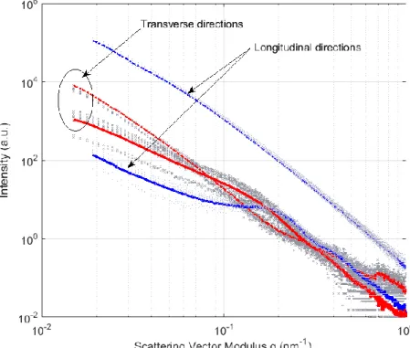
x profiles shown in Figs. 7 and 8, this question has been addressed. In what follows, I q( ) profiles are indexed according to the SAXS image axis that corresponds either to the longitudinal (tensile) or transverse directions to make interpretations more straightforward.

In Fig. 9 we have placed the average I q( ) profiles extracted from the SAXS patterns associated with different material points but for which the strain was almost exactly 0.15

and 1.5. Going back to Fig. 2 where the SAXS patterns are represented by dots, those

which were selected for Fig. 9 are comprised between envelope curves corresponding respectively to 0.150.02 and 1.50.02. For each strain level, about 50 SAXS patterns

were found in this uncertainty range. The intensity curves taken along the longitudinal direction are in blue and those associated with the transverse directions are in red (identified by arrows). The curves associated with 0.15 are shown as full lines and those

corresponding to 1.5 are shown as dotted lines. To make this figure clearer, we only show

in light grey a few representative profiles chosen among the 50 curves used to calculate the

Pre-refereeing

version

published

in JPSB

average curve. At a high strain level (1.5), all the curves lie very close together and are

centered around the average curve. This demonstrates that the constant values observable for the A x_

 

curves at high strain levels in Fig. 7 or Fig. 8 are indeed the signatures of a unique anisotropy state. For lower strain levels (0.15), all the curves are very similar but

are more scattered around the average profiles. This is logical when one considers that material points with a small strain level can be found at various positions but systematically in regions straight ahead of strong specimen curvatures (in the center of the specimen at the beginning of the test, in the shoulder at the end of the test). This will be demonstrated as a triaxiality effect in the final section and explains the moderate variations that can be seen on the A x_

 

curves at low strain levels in Fig. 7 or Fig. 8.

Figure 9: Average longitudinal and transverse intensity curves versus reciprocal vector magnitude for two strain levels 0.15 (solid lines) and 1.5(dotted lines). Gray curves are

for a few representative examples of those profiles obtained for different material points X at same strains, which enter into the averaging; see text for details.

Thanks to the large amount of data obtained in a single experiment, and with the same procedure, it is possible to produce noise reduced I

 

q profiles for a multiple strain state. Depending on a given strain level  defined at 0.02, an amount between 15-50

Pre-refereeing

version

published

in JPSB

SAXS images can be associated with this strain level but for different material points. considering the undeformed state ( 0), the I

 

q profile was obtained by averaging over 516 patterns corresponding to the first and the last acquistion during each of the 208 scans. These patterns correspond to material grains in quasi-undeformed areas of the specimen all over the tensile test. In Fig. 10 and Fig. 11 we show the averageI

 

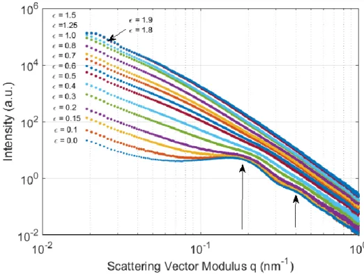
q curves respectively taken along the longitudinal (Fig. 10) and the transverse (Fig. 11) directions for different strain levels. By comparing with the non averaged curves (light grey in Fig. 9), the noise reduction appears clearly at low strain levels in particular in the region of high q values.

For  0, we obtained the long period of lamellae stacks by calculating the central

position of the peaks in the



q q2I



, representation (see Fig.1 in supplementary information file) with the equation: peak

q

d2 . From the longitudinal profiles, the calculated value corresponds to the peridiocity measured for the stacks of lamellae with a normal vector perpendicular to the tensile direction. From the transverse profiles we recover the long period associated with the stacks of lamellae which are oriented with a normal vector along the tensile direction.

In the longitudinal direction (Fig. 10), the intensity profiles are placed according to a logical sequence depending on the strain level  . At low strain levels, the peak associated with the long period of the lamellae stack is clearly visible in Fig. 10 (arrows). The secondary correlation peak is also easy to detect, which can be problematic in the presence of high noise levels (Schneider, 2006). It can also be seen that when the strain increases, the peak moves towards a higher q value, which corresponds to a decrease of the long period of the

stacks of lamellae that are parallel to the tensile axis: the lamellae come close to each other.

Pre-refereeing

version

published

in JPSB

Figure 10: Intensity versus reciprocal vector magnitude in the longitudinal direction plotted for different strain levels

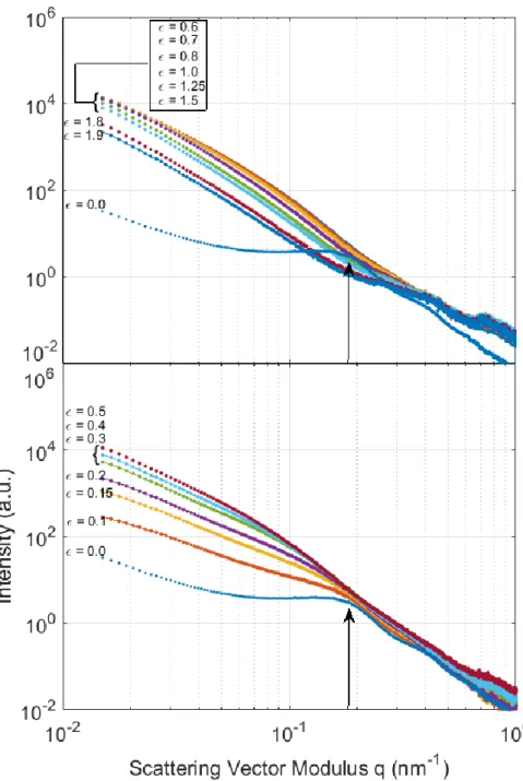
In the transverse direction (Fig. 11), intensity profiles show the same peak for  0

provided that for 0.1, because of intense scattering coming from the nanovoids, the peak

is partly blurred and replaced by a shoulder. This shoulder moves towards lower q values

with increasing strain (Fig. 11 lower panel); the long period of the stacks of lamellae oriented perpendicularly to the the tensile axis increases when the strain increases. All the curves are perfectly ordered with an overall increase in intensity. For  0.5 0.6 (Fig.11 upper panel), the profiles do not evolve in shape and they are perfectly ordered with overall decreasing intensity.

For 0.4, no peak or shoulder is distinguishable on any profile because: i) the

lamellar morphology has begun to be destroyed and ii) the intensity scattering resulting from the lamellae/amorphous density difference becomes very small relative to the scattering coming from nanovoids. Comparable results have been observed previously (Xiong, 2014; Schneider, 2006; Butler, 1997).

Pre-refereeing

version

published

in JPSB

Figure 11: Intensity versus reciprocal vector magnitude in the transverse direction plotted for different strain levels (lower panel 0  0.5 , upper panel 0.6  1.9).

Pre-refereeing

version

published

in JPSB

4. ANALYSIS OF THE THICKNESS DEPENDENCY OF THE DEFORMATION STATE

The major objective of this section is to demonstrate that variations of the A x_

 

profiles, observable in Fig. 7 for the curves corresponding to 1.2, can be consistently

explained by considering that the strain is not constant along the thickness direction when the specimen shows a local significant curvature. The curved parts of the specimen are first situated in the neighborhood of the neck center at the beginning of the plastic deformation process. Next, the central part of the specimen becomes flat, with a strain of 2 and the

most curved regions are situated in the neck shoulders (see Fig. 3, this paper and Fig. 10 Ye et al., 2015).The DIC technique can only provide a surface measurement, while the anisotropy index is a volume measurement since the X-ray beam crosses the specimen thickness.

First we will focus on significant variations of A_

 

x that take place in the



5,5



mm range with the specific features that can be described as follows:

 At low strain levels



0.1



, a strong decrease of the A0.1

 

x curve associated with a strong slope change can be observed in the x range considered:





0.1 5 0.4

A_ x  mm   , while A0.1

 

x0 0.65.

 When the strain increases, the curve drop becomes less pronounced: it is still visible for



0.15



but the curve is nearly flat at 0.2.

 Next, for 0.3, the trend is clearly in the opposite direction: the A0.3

 

x curve

increases for x 3mm and reaches a maximum at x0. For 0.5 or 0.6, the

curve increases in the central region ( x 3mm) being very pronounced.

 For larger strain levels, the effect is progressively less marked to become hardly noticeable for 1.

In the following section, we show that Finite Element (FE) modelling of the experiment can provide interesting information to interpret this set of observations. We used the Abaqus® software with C3D10 elements (quadratic tetrahedral elements). Using symetries, it was possible to only model 1/8th of the specimen. The meshing is shown in Fig. 12a for the HDPE6 geometry. The plastic behavior of the material was deduced through the true stress/true strain curve (see Fig.2 in supplementary information file) that was measured in

Pre-refereeing

version

published

in JPSB

the center of the neck (see Farge et al. 2013 for the procedure). In this work, the FE modelling of the tensile experiment was only carried out up to moderate strain levels. The complete FE modelling of the deformation process of a semi-crystalline polymer specimen up to very large strain levels (e.g 2) would be a very challenging task that, as far as we

know, has never been achieved. In particular, it would be necessary to describe correctly the second plastic instability occurring during the deformation process at 1.2 in the specimen

center for our material (Ye et al., 2015). Physically, the second plastic instability corresponds to the propagation of the neck towards the nondeformed region of the specimen in response to the grip displacement. This step is necessary to allow the progressive stabilization of the deformation process with finally cte2 in the specimen center. Our FE

results are shown in Fig. 12b,c for Smax0.10 and 0.3

max_

S

 . max

S

 is the maximum longitudinal strain on the specimen front face where the DIC measurement is performed. Note that this is not the maximum strain over the whole specimen: the strain can be larger in the specimen core.

Figure 12: (a) Meshing of the HDPE6 specimen - FE results obtained for a maximum longitudinal strain of Smax0.10 (b) and 0.30

max_

S

 (c) on the front specimen face (DIC measurement surface).

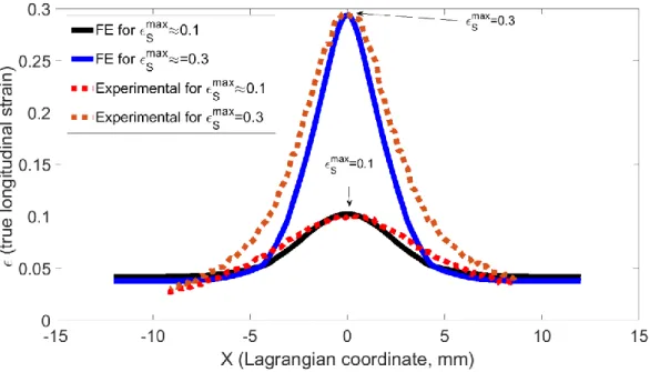
To compare the FE results with those of the DIC experiments, we have plotted in Fig. 13 the strain along a longitudinal central line (x-axis). For Smax0.3, the obtained

Pre-refereeing

version

published

in JPSB

experimental and FE curves show the same trends but it can be seen that the width of the neck given by the FE modelling is somewhat underestimated. For max0.1

S

 , the agreement between the experimental results and the simulation is much better. This allows us to consider that our FE results show sufficient agreement with the experimental results that they can be used to perform a semi-quantative analysis of SAXS measurements.

Figure 13: Longitudinal 

 

X profiles along longitudinal path L (see Fig 12-a)

In Fig. 14, we show two strain profiles plotted, respectively, along path A (Fig. 12a,

0

x ) and path B (Fig. 12b, x3.5mm). For the surface points belonging to these two paths, where the DIC measurement is obtained, the strain level is the same: 0.10. The following

points can be noted:

 In the case of path A, the strain in the material core is significantly higher than on its surface; the mean value calculated over path A is 0.117

A

  . This strain heterogeneity with the exact same trend has been shown by numerous authors and also using FE methods, when modelling plastic deformation processes of ductile materials (Mikkelsen, 1999; Li, 2010). As a result, when the X-ray beam travels along path A, it probes a strain larger than that “measured” at this time by DIC. In Fig. 7, the anisotropy factor corresponding to this strain is A_0.1



x0



0.65.

Pre-refereeing

version

published

in JPSB

 In contrast, along path B situated at x 3.5mm, the mean strain is smaller than 0.10:

0.073

B

  and A_0.1



x 3.5mm



 0.56. This corresponds to a drop in the anisotropy index 0.09

A

   , which we attribute to the difference of the mean  value between the two cases. For 0.073  0.117, the anisotropy curves are clearly in their decreasing zone (see

Figs. 5 or 6). As an illustration, in Fig. 6 for

X



0

and for    _A the anisotropy index is roughly A_{X 0}



0.073



 0.6. In contrast, for

B 

  the anisotropy index is roughly





0 0.117 0.7

X

A _    . This corresponds to a drop of the anisotropy index A0.10,

which fits approximately with the anisotropy index drop that we observe between

3.5

x  mm and x0 in Fig. 7 for the 0.1 curve.

 Along Path C taken at x0 (Fig. 12c), the surface strain is 0.3 but in the core, it can be

seen that it is slightly higher 0.4. The average strain along Path C is then  _C0.37. In that case, again the mean strain probed by the X-ray beam when it passes through the center of the neck (x0) is larger than that measured at this time and used to index the

anisotropy curves. For this strain level (0.3) the anisotropy curve is clearly in its

increasing region (Figs. 5 or 6). This explains the anisotropy index increase that is observed for 0.3 in the part of the curve close to x0 (Fig. 7). The same explanation

holds for explaining the anisotropy index increase in the x 3mm that is observable up to 1.2 in Fig. 7.

Pre-refereeing

version

published

in JPSB

Figure 14: Through-thickness 

 

Z profiles along path A and B (see Fig 12(b and c)).

Pre-refereeing

version

published

in JPSB

At this point of the analysis, the strain heterogeneity calculated by FE modelling for low strain values fully explains all specific features of the A

 

x curves of Fig. 7: transition from a strong decrease of the anisotropy index for x5mm and for 0.2 to an increase for 0.2.

This highlights the importance of the point of the maximum transverse anisotropy, at 0.2

in our case and clearly put forward the role of triaxiality to explain the scattering of the data presented before. As has already been discussed, for higher strains the neck becomes very flat in its center. There the stress state is “quasi-uniaxial” and the strain is nearly constant when the X-ray beams cross the specimen. Furthermore, at high strain levels, the dependence of anisotropy index variations on the strain becomes much less pronounced (Fig. 5). As a result, for 1.2 the anisotropy profiles become constant (Figs. 7 and 8).

FE modelling was also performed for the HDPE3 specimen and we again observed that at the beginning of the deformation process, the strain was significantly larger in the specimen core than on its surface. For HDPE3, the mean strain value is  _C0.36 along a path corresponding to path C (i.e path in the neck center with 0.3 on the surface). This value is very close to the  _C0.37 value found for HDPE6 along path C. The same applies to paths corresponding to paths A and B, where we found respectively for HDPE3 the values

0.076

A

 and  _B0.113. This explains that the curves are nearly perfectly superimposed for HDPE3 and HDPE6 in Fig.5.

Lastly, concerning the x5mm region where the A( x) curves also exhibit some variations, the same explanation holds. These points correspond during a great part of the tensile test to material grains in the neck shoulder where strain heterogeneities and stress triaxiality are present. For example, if we focus on a point at x7mm with 0.6, the running time of the experiment is t700s. Re-examining Fig. 4 shows that at this time, the central RVE is almost in the maximum deformed state of 2. Hence this point is clearly in the neck

shoulder where strain heterogeneities are present. In light of this analysis, the variations of the A_( x) curves for all strains below 1.2 and the whole x-range both result from the

different cross-section averaged strain values probed by the beam.

Pre-refereeing

version

published

in JPSB

5. CONCLUSION

Our results can be summarized as follows. The different material points of tensile deformed HDPE specimens are subjected to various deformation paths as a consequence of plastic instability onset and development in a dog-bone shaped specimen. However, based on full field 1D SAXS measurements, we show that the true (Hencky) strain governs the current topology of the microstructure characterized through an anisotropy index. This index is the reflection of the complex reorganizations occurring in the bulk, to pass from the randomly oriented lamellar stack organization to a fibrillar state, as imposed by the drawing. It shows an anisotropy that develops first in the transverse direction (up to a strain of 0.15) and then reverses to recover an isotropy state around a strain of 0.6 and further develops toward a fully fibrillar state. This path is shown to hold for any material point, irrespective of its deformation path. The proof is given through the analysis of two distinct behaviors as highlighted by anisotropy profiles. At high strain levels, namely 1.2, anisotropy profiles are completely flat; the microstructure state is completely independent of the deformation path and depends only on current longitudinal strain. For the lower strain levels, anisotropy profiles can depart from this flat behavior. These small deviations have been characterized approximately, thanks to a FE solution. They are obviously shown as the result of strain heterogeneities or triaxiality effects that exist only at these special times and positions where the beam crosses regions with strong specimen curvatures. As the anisotropy profiles are indexed by the strain measured at the surface specimen, but are produced from SAXS bulk investigations, apparent discrepancies result. Realistic FE simulations in the presence of plastic instabilities are still a challenging task, but in the light of this work would be of prime importance to define average bulk strains in an exact manner to define deformation states which are not characterized by a surface measurement only.

Pre-refereeing

version

published

in JPSB

REFERENCES

Galeski, A. Strength and toughness of crystalline polymer systems. Prog. Polym. Sci. 2003, 28 (12), 1643-1699.

Butler, M.F.; Donald, A.M.; Brass, W.; Mant, G.R.; Derbyshire, G.E.; Ryan, A.J. A Real-Time simultaneous small- and wide-angle X-ray scattering study of In-Situ deformation of isotropic polyethylene Macromolecules 1995, 28, 6383-6393.

Butler, M.F.; Donald, A.M.; Ryan, A.J. Time resolved simultaneous small- and wide-angle X-ray scattering during polyethylene deformation – I Cold drawing of ethylene--olefin copolymers Polymer 1997, 38 (22), 5521-5538.

Butler, M.F.; Donald, A.M. Deformation of spherulitic polyethylene thin films. J. of Materials

Science 1997, 32, 3675-3685.

Schneider, K.; Trabelsi, S.; Zafeiropoulos, N.E.; Davies, R.; Riekel, Chr.; Stamm, M. The Study of Cavitation in HDPE Using Time Resolved Synchrotron X-ray Scattering During Tensile Deformation. Macromol. Symp. 2006, 236, 241–248.

Humbert, S.; Lame, O.; Chenal, J.M.; Rochas, C.; Vigier, G. New Insight on Initiation of Cavitation in Semicrystalline Polymers: In-Situ SAXS Measurements Macromolecules 2010, 43, 7212–7221.

Rozanski, A.; Galeski, A.; Debowska, M. Initiation of Cavitation of Polypropylene during tensile drawing Macromolecules 2011, 44(1), 20–28.

Schneider, K. Investigation of Structural Changes in Semi-Crystalline Polymers During Deformation by Synchrotron X-Ray Scattering. J. Polymer Sc. Part B-Polymer Physics 2010, 48(14), 1574-1586.

Jiang, Z.; Tang, Y.; Men, Y. Structural evolution of tensile-deformed high-density polyethylene during annealing: Scanning synchrotron small-angle X-ray scattering study.

Macromolecules 2007, 40(20), 7263-7269.

Xiong, B.; Lame, O.; Chenal, JM.; Rochas, C.; Seguela, R.; Vigier, G. In-situ SAXS study of the mesoscale deformation of polyethylene in the pre-yield strain domain: Influence of microstructure and temperature Polymer 2014, 55(5), 1223–1227.

Zhao, J.; Sun, Y.; Men, Y. Elasticity Reinforcement in Propylene-Ethylene Random Copolymer Stretched at Elevated Temperature in Large Deformation Regime Macromolecules 2016, 49 (2), 609-615.

Pre-refereeing

version

published

in JPSB

André, S.; Meshaka, Y.; Cunat, C. Rheological constitutive equation of solids : a link between models based on irreversible thermodynamics and on fractional order derivative equations

Rheologica Acta, 2003, 42, 500-515.

Blaise, A.; André, S.; Delobelle, P.; Meshaka, Y.; Cunat, C. Advantages of a 3-parameter Reduced Constitutive Model for the Measurement of Polymers Elastic Modulus using Tensile Tests. Mechanics of Time-Dependent Materials 2016, 20(4), 553-577.

Farge, L.; André, S.; Meneau, F.; Dillet, J.; Cunat, C. A common multiscale feature of the deformation mechanisms of a semi-crystalline polymer Macromolecules 2013, 46(24), 9659-9668.

Blaise, A.; Baravian, C.; Dillet, J.; Michot, L.J.; André, S. Characterization of the mesostructure of HDPE under “in-situ” uniaxial tensile test by incoherent polarized steady-light transport, Journal of Polymer Science B: Polymer Physics 2011, 50(5), 328–337.

Farge, L.; Boisse, J.; Dillet, J.; André, S.; Albouy, P-A; Meneau, F. WAXS study of the lamellar/fibrillar transition for a semi-crystalline polymer deformed in tension in relation with the evolution of volume strain Journal of Polymer Science, B Polymer Physics 2015, 53, 1470–1480.

Henrich, B.; Bergamaschi, A.; Broennimann, C.; Dinapoli, R.; Eikenberry, E. F.; Johnson, I.; Kobas, M.; Kraft, P.; Mozzanica, A.; Schmitt, B., PILATUS: A single photon counting pixel detector for X-ray applications Nuclear Instruments and Methods in Physics Research Section

A 2009, 607 (1), 247-249 (10.1016/j.nima.2009.03.200).

Blaise, A.; Baravian, C.; André, S.; Dillet, J.; Michot, L.J.; Mokso, R. Investigation of the mesostructure of a mechanically deformed HDPE by synchrotron microtomography,

Macromolecules, 2010, 43, 8143-8152.

Ye, J.; Andre, S.; Farge, L. Kinematic Study of Necking in a SemiCrystalline Polymer through 3D Digital Image correlation Int. J. Solids & Structures 2015, 59, 48-72.

Pawlak, A. Cavitation during tensile deformation of high-density polyethylene. Polymer 2007,

48, 1397-1409.

Castagnet, S.; Girault, S.; Gacougnolle, J.L.; Dang, P. Cavitation in strained polyvinylidene fluoride: mechanical and X-ray experimental studies. Polymer 2000, 41, 7523-7530.

Pawlak, A.; Galeski, A. Cavitation during Tensile Deformation of Polypropylene.

Macromolecules 2008, 41, 2839-2851.

Zhang, X.; Schneider, K.; Liu, G.; Chen, J.; Brüning, K.; Wang, D.; Stamm, M. Deformation-mediated superstructures and cavitation of poly (L-lactide): In situ small-angle X-ray scattering study. Polymer 2012, 53, 648-656.

Pre-refereeing

version

published

in JPSB

Laiarinandrasana, L.; Klinkova, O.; Nguyen, F.; Proudhon, H.; Morgeneyer, T.F.; Ludwig, W. 2016, Three dimensional quantification of anisotropic void evolution in deformed semi-crystalline polyamide 6, International Journal of Plasticity 2016, 83, 19-36.

Xiong, B.; Lame, O.; Chenal, J. M.; Rochas, C.; Seguela, R.; Vigier, G. In-situ SAXS study and modeling of the cavitation/crystal-shear competition in semi-crystalline polymers: Influence of temperature and microstructure in polyethylene. Polymer 2013, 54(20), 5408-5418.

Mikkelsen, L.P. Necking in rectangular tensile bars approximated by a 2-D gradient dependent plasticity model. Eur. J. Mech.A/Solids 1999, 18, 805-818.

Li, H.X.; Buckley, C.P. Necking in glassy polymers: Effect of intrinsic anisotropy and structural evolution kinetics in their viscoplastic flow. International Journal of Plasticity 2010, 26, 1726-1745.

Pre-refereeing

version

published

in JPSB

Supplementary information

Figure 1: related to section "I(q) Intensity curves" which gives a



q,q2I



plot to determine the

position of correlation peaks.

Pre-refereeing

version

published

in JPSB

Figure 2: related to section 4 which gives the true stress-true strain curve of the HDPE material studied in the paper.

Pre-refereeing

version

published

in JPSB