Comparison of Artificial Intelligence Techniques for river flow forecasting

(1)

HAL Id: hal-00305124

https://hal.archives-ouvertes.fr/hal-00305124

Submitted on 30 Jan 2008

HAL is a multi-disciplinary open access

archive for the deposit and dissemination of

sci-entific research documents, whether they are

pub-lished or not. The documents may come from

teaching and research institutions in France or

abroad, or from public or private research centers.

L’archive ouverte pluridisciplinaire HAL, est

destinée au dépôt et à la diffusion de documents

scientifiques de niveau recherche, publiés ou non,

émanant des établissements d’enseignement et de

recherche français ou étrangers, des laboratoires

publics ou privés.

flow forecasting

M. Firat

To cite this version:

M. Firat. Comparison of Artificial Intelligence Techniques for river flow forecasting. Hydrology and

Earth System Sciences Discussions, European Geosciences Union, 2008, 12 (1), pp.123-139.

�hal-00305124�

(2)

Hydrol. Earth Syst. Sci., 12, 123–139, 2008 www.hydrol-earth-syst-sci.net/12/123/2008/ © Author(s) 2008. This work is licensed under a Creative Commons License.

Hydrology and

Earth System

Sciences

Comparison of Artificial Intelligence Techniques for river flow

forecasting

M. Firat

Research Assistant (PhD), Pamukkale University Civil Engineering Department, Denizli, Turkey Received: 15 May 2007 – Published in Hydrol. Earth Syst. Sci. Discuss.: 6 June 2007

Revised: 15 October 2007 – Accepted: 20 December 2007 – Published: 30 January 2008

Abstract. The use of Artificial Intelligence methods is

be-coming increasingly common in the modeling and forecast-ing of hydrological and water resource processes. In this study, applicability of Adaptive Neuro Fuzzy Inference Sys-tem (ANFIS) and Artificial Neural Network (ANN) methods, Generalized Regression Neural Networks (GRNN) and Feed Forward Neural Networks (FFNN), and Auto-Regressive (AR) models for forecasting of daily river flow is investigated and Seyhan River and Cine River was chosen as case study area. For the Seyhan River, the forecasting models are es-tablished using combinations of antecedent daily river flow records. On the other hand, for the Cine River, daily river flow and rainfall records are used in input layer. For both stations, the data sets are divided into three subsets, training, testing and verification data set. The river flow forecasting models having various input structures are trained and tested to investigate the applicability of ANFIS and ANN and AR methods. The results of all models for both training and test-ing are evaluated and the best fit input structures and methods for both stations are determined according to criteria of per-formance evaluation. Moreover the best fit forecasting mod-els are also verified by verification set which was not used in training and testing processes and compared according to criteria. The results demonstrate that ANFIS model is supe-rior to the GRNN and FFNN forecasting models, and ANFIS can be successfully applied and provide high accuracy and reliability for daily river flow forecasting.

1 Introduction

In last decades, the forecasting and modeling of river flow in hydrological processes is quite important to deliver the sustainable use and effective planning and management of Correspondence to: M. Firat

(mfirat@pamukkale.edu.tr)

the water resources. In order to estimate hydrological pro-cesses such as precipitation, runoff and change of water level by using existing methods, some parameters such as the physical properties of the watershed and river network and observed detail data are necessary. In the literature, there have been many approaches such as, Box and Jenkins (1970) methods of autoregressive (AR), auto-regressive moving av-erage (ARMA), auto-regressive integrated moving avav-erage (ARIMA), autoregressive, moving average with exogenous inputs (ARMAX), generally used for modeling of river flow. Some of the earliest examples of the AR type of stream flow forecast models include Thomas and Fiering (1962) and Yev-jevich (1963). These approaches have employed conven-tional methods of the time series forecasting and modeling (Owen et al., 2001; BuHamra et al., 2003; Zhang, 2003; Mo-hammadi et al., 2006; Arena et al., 2006; Komornik et al., 2006; Toth et al., 2000). Artificial neural networks (ANN) have been recently accepted as an efficient alternative tool for modeling of complex hydrologic system to the conventional methods and widely used for prediction. Some specific ap-plications of ANN to hydrology include modeling rainfall-runoff process (Sajikumar et al., 1999), river flow forecast-ing (Dibike et al., 2001; Chang et al., 2002; Sudheer and Jain; 2004; Dawson et al., 2002), sediment transport predic-tion (Firat and G¨ung¨or, 2004), and sediment concentrapredic-tion estimation (Nagy et al., 2002). The ASCE Task Commit-tee reports (2000) did a comprehensive review of the appli-cations of ANN in hydrological forecasting context. Jain and Kumar (2007) proposed a new hybrid time series neu-ral network model that is capable of exploiting the strengths of traditional approaches and ANN. Tingsanchali and Gau-tam (2000) applied ANN and stochastic hydrologic models to forecast the flood in two river basins in Thailand. GRNN method have also been used for many specific studies (Ci-gizoglu, 2005; Cigizoglu and Alp, 2006; Kim et al., 2004; Ramadhas et al., 2006; Celikoglu and Cigizoglu, 2007; Ce-likoglu, 2006). On the other hand, Fuzzy Logic (FL) method

(3)

OUTPUT Fuzzification Decision System Defuzzification Database Rulebase Knowledge Base INPUT

Fig. 1: The General Structure of fuzzy Inference System

∏ ∏ + = + = μ μ μ μ

Fig. 1. The general structure of the Fuzzy Inference System.

was first developed to explain the human thinking and de-cision system by Zadeh (S¸en, 2001). Several studies have been carried out using fuzzy logic in hydrology and water resources planning (Chang et al., 2001; Liong et al., 2000; Mahabir et al., 2000; Nayak et al., 2004a; S¸en and Altunkay-nak, 2006). Recently, Adaptive Neuro-fuzzy inference sys-tem (ANFIS), which consists of the ANN and FL methods, have been used for several application such as, database man-agement, system design and planning/forecasting of the wa-ter resources (Chen et al., 2006; Chang et al., 2006; Nayak et al., 2004b; Firat, 2007; Firat and G¨ung¨or, 2007; Kisi, 2006). The main purpose of this study is to investigate the ap-plicability and capability of ANFIS, ANN and AR methods for modeling of daily river flow. To verify the application of these approaches, two case study areas, Seyhan River and Cine River, were chosen. For the Seyhan River, daily river flow records measured at the time period 1986–2000 years are used to establish the river flow forecasting models. For the Cine River, daily river flow and rainfall records measured between 1992–2000 years are used. For both case study, all models are trained and tested and performances of mod-els are compared with observation records. The best fit in-put structure and method is determined according to perfor-mances. Then the best fit models for Seyhan River and Cine River is verified using verification data set to evaluate the performances of models.

2 Adaptive Neuro Fuzzy Inference System (ANFIS)

The FL approach is based on the linguistic uncertainly

ex-pression rather than numerical uncertainty. Since Zadeh

(1965) proposed the FL approach to describe complicated systems, it has become popular and has been successfully used in various engineering problems, (Chen et al., 2006; Chang et al., 2001; Liong et al., 2000; Mahabir et al., 2000; Nayak et al., 2004a; Firat, 2007; Nayak et al., 2004b; S¸en, 2001). Fuzzy inference system (FIS) is a rule based sys-tem consists of three conceptual components. These are: (1) a rule-base, containing fuzzy if-then rules, (2) a data-base, defining the Membership Function (MF) and (3) an inference system, combining the fuzzy rules and produces the system results (S¸en, 2001). The first phase of FL modeling is the determination of MFs of input –output variables, the second

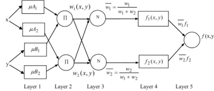
y x ∏ ) , ( 1 xy w ∏ N N ) , ( 2 x y w 1 1f w 2 2f w

Layer 1 Layer 2 Layer 3 Layer 4 Layer 5

2 1 1 1 _w _w w w + = 2 1 2 2 w w w w + = 1 A μ 2 A μ 1 B μ 2 B μ ) , ( 1xy f ) , ( 2xy f f (x,y)

Fig. 2: The Scheme of ANFIS

Fig. 2. The scheme of Adaptive Neuro-Fuzzy Inference System.

phase is the construction of fuzzy rules and the last phase is the determination of output characteristics, output MF and system results. A general structure of fuzzy system is demon-strated in Fig. 1.

ANFIS consisting of the combination of the ANN and the FL has been shown to be powerful in modeling numer-ous processes such as rainfall-runoff modeling and real-time reservoir operation (Chen et al., 2006; Chang et al., 2006; Firat and G¨ung¨or, 2007). ANFIS uses the learning ability of ANN to define the input-output relationship and construct the fuzzy rules by determining the input structure. The system results were obtained by thinking and reasoning capability of the fuzzy logic. There are two types of FISs, Sugeno-Takagi FIS and Mamdani FIS, in literature. In this study, Sugeno Takagi FIS is used for modeling of daily river flow. The most important difference between these systems is the definition of the consequent parameter. The consequence pa-rameter in Sugeno FIS is a linear equation, called first-order Sugeno FIS, or constant coefficient, zero-order Sugeno FIS (Jang et al., 1997). It is assumed that the fuzzy inference system includes two inputs, x and y, and one output, z. For the first-order Sugeno FIS, typical two rules can be expressed as;

Rule 1: IF x is A1and y is B1

THEN f1=p1∗x + q1∗y + r1

Rule 2: IF x is A2and y is B2

THEN f2=p2∗x + q2∗y + r2

where, x and y are the crisp inputs to the nodei, Ai and Bi

are the linguistic labels as low, medium, high, etc., which are

characterized by convenient MFs and finally, pi, qi and ri

are the consequence parameters. The structure of this FIS is shown in Fig. 2.

Input notes (Layer 1): Each node in this layer generates membership grades of the crisp inputs which belong to each of convenient fuzzy sets by using the MFs. Each node’s

out-put O_i1is calculated by:

O_i1=µAi(x) for i = 1, 2

(4)

M. Firat: Comparison of Artificial Intelligence Techniques for river flow forecasting 125

where µAi and µBi are the MFs for Ai and Bifuzzy sets,

respectively. In this study, the Gauss MF is used, as;

O_i1=µAi(x) = e

−(x−c)2

2σ 2 ₍₂₎

Rule nodes (Layer 2): In this layer, the AND/OR opera-tor is applied to get one output that represents the results of the antecedent for a fuzzy rule, that is, firing strength. The

outputs of the second layer, called firing strengths O_i2, are

the products of the corresponding degrees obtained from the layer 1, named as w as follows;

O_i2=wi =µAi(x)µBi(y), i = 1, 2 (3)

Average nodes (Layer 3): Main target is to compute the ra-tio of firing strength of each ith rule to the sum firing strength of all rules. The firing strength in this layer is normalized as;

O_i3= ¯wi = wi P i wi i = 1, 2 (4)

Consequent nodes (Layer 4): The contribution of it hrule towards the total output or the model output and/or the func-tion defined is calculated by Eq. (5);

O_i4= ¯wifi = ¯wi(pix + qiy + ri) i = 1, 2 (5)

¯

wi is the ith node output from the previous layer as

demon-strated in the third layer. {pi, qi, ri} is the parameter set in

the consequence function and also the coefficients of linear combination in Sugeno inference system.

Output nodes (Layer 5): This layer is called as the output nodes in which the single node computes the overall output by summing all incoming signals and is also the last step of the ANFIS. The output of the system is calculated as;

f (x, y) =w1(x, y)f1(x, y) + w2(x, y)f2(x, y) w1(x, y) + w2(x, y) =w1f1+w2f2 w1+w2 (6) Q5_i =f (x, y) =X i ¯ wi.fi = ¯wif1+ ¯wif2= P i wifi P i wi (7)

The objective is to train adaptive networks for having conve-nient unknown functions given by training data and finding the proper value of the input and output parameters. For this aim, ANFIS applies the hybrid-learning algorithm, consists of the combination of the “gradient descent” and “the least-squares” methods. The gradient descent method is used to assign the nonlinear input parameters, as the least-squares method is employed to identify the linear output parame-ters. The detailed algorithm and mathematical background of these algorithms can be found in Jang et al. (1997).

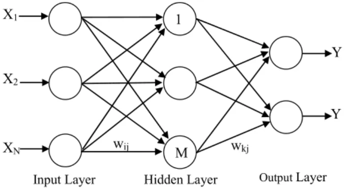
X1 X2 XN 1 M Y Y

Input Layer Hidden Layer Output Layer

wkj

wij

Fig. 3: General Structure of a FFNN

Fig. 3. General structure of a FFNN.

3 Artificial Neural Networks

An ANN can be defined as a system or mathematical model consisting of many nonlinear artificial neurons running in parallel which can be generated as one or multiple layered. In this study, GRNN and FFNN methods are used for fore-casting of daily river flow.

3.1 Feed Forward Neural Networks (FFNN)

A FFNN consists of at least three layers, input, output and hidden layer. The number of hidden layers and neurons in hidden layer are determined by trial and error method. The schematic diagram of a FFNN is shown in Fig. 3. Each neu-ron in a layer receives weighted inputs from a previous layer and transmits its output to neurons in the next layer. The summation of weighted input signals is calculated by Eq. (8) and is transferred by a nonlinear activation function given in Eq. (9). The responses of network are compared with the observation results and the network error is calculated with Eq. (10). Ynet= N X i=1 Xi.wi+w0 (8) Yout=f (Ynet) = 1 1 + e−Ynet (9) Jr = 1 2. k X i=1 (Yobs−Yout)2 (10)

Yout is the response of neural network system, f (Ynet) is

the nonlinear activation function, Ynet is the summation of

weighted inputs, Xi is the neuron input, wi is weight

coef-ficient of each neuron input, w0 is bias, Jr is the error

be-tween observed value and network result, Yobs is the

obser-vation output value. In this study, the back propagation learn-ing algorithm, the supervised learnlearn-ing and sigmoid activation function are used in training and testing of models.

(5)

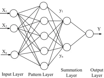
Input Layer Pattern Layer Summation _Layer Output _Layer X1 X2 Xn Y y1 yn

Fig. 4: The General Structure of a GRNN

Fig. 4. The general structure of a GRNN.

3.2 Generalized Regression Neural Networks (GRNN)

A GRNN is a variation of the radial basis neural networks, which is based on kernel regression networks (Cigizoglu, 2005; Cigizoglu and Alp, 2006). A GRNN doesn’t require an iterative training procedure as back propagation networks. A GRNN consists of four layers: input layer, pattern layer, summation layer and output layer as shown in Fig. 4.

The number of input units in input layer depends on the total number of the observation parameters. The first layer is connected to the pattern layer and in this layer each neuron presents a training pattern and its output. The pattern layer is connected to the summation layer. The summation layer has two different types of summation, which are a single division unit and summation units. The summation and output layer together perform a normalization of output set. In training of network, radial basis and linear activation functions are used in hidden and output layers. Each pattern layer unit is connected to the two neurons in the summation layer, S and D summation neurons. S summation neuron computes the sum of weighted responses of the pattern layer. On the other hand, D summation neuron is used to calculate unweighted outputs of pattern neurons. The output layer merely divides the output of each S-summation neuron by that of each D-summation neuron, yielding the predicted value to an un-known input vector x as (Kim et al., 2004);

Y_i′= n P i=1 yi. exp [−D(x, xi)] n P i=1 exp [−D(x, xi)] (11) D(x, xi) = m X k=1 (xi−xik σ ) 2 ₍₁₂₎

yi is the weight connection between the ith neuron in the

pattern layer and the S-summation neuron, n is the number

of the training patterns, D is the Gaussian function, m is the

number of elements of an input vector, xkand xikare the j th

element of x and xi, respectively, σ is the spread parameter,

whose optimal value is determined experimentally.

4 Auto-Regressive Model

In the traditional analysis techniques, the data set must be di-vided to periodical component, trend component, internal de-pendent component and indede-pendent (random) components. Trend is the evidence of the increase or decrease of process parameters (mean and standard deviation) by time. It is un-derstood that there is a periodical component when the pa-rameters of the process show variation in a determined pe-riod. BOX-COX transformation was applied to the data to converge the data to normal distribution. The periodicity of the daily means and standard deviations were calculated by using Fourier series to arrange the periodicity in the data.

DN Y (t ) = DY (t ) − DY

σDY

(13) where DN Y (t ) is the normalized time series variable, DY (t ) is the original time series variable, DY is the mean of the

original time series data and σDY is the standard deviation

of the original time series data. In order to get more accu-rate and reliable evaluation and comparison the best fit input structures were used to forecast the daily river flow by using AR models. The structure of AR model for Seyhan River and ARX (Auto Regressive with eXogenous inputs) model for Cine River was given in Eqs. (14) and (15).

Q(t ) = N X i=1 αiQ(t − i) + ε(t ) (14) Q(t ) = N X i=1 αiQ(t − i) + m X k=1 αkP (t − k) + ε(t ) (15)

where, Q(t) is the daily river flow, Q(t−i) is the river flow at (t−i) time, αis the auto-regressive parameter to be de-termined (i) is an index representing the order of AR model,

P (t −k) is the rainfall at (t−k) time, αkis the auto-regressive

parameter and ε(t ) is the random error. The optimal values of ARX model parameters were estimated using the MATLAB Identification Toolbox and identification data set. The model parameters are selected using Akaike’s final prediction error (FPE) criterion.

5 Study area and available data

To illustrate the applicability of the ANFIS and ANN meth-ods, two river stations, Seyhan River and Cine River, were chosen as case study. Seyhan River, located in South of

(6)

M. Firat: Comparison of Artificial Intelligence Techniques for river flow forecasting 127 • − − − • • • • • •

Fig. 5. Study areas.

is chosen as case study area. Seyhan River has lengthy of

560 km and the drainage area of 20 600 km2. Climatic

condi-tions in the area are typical Mediterranean climate and annual average rainfall is 600 mm. There are two big dams, Seyhan and Catalan, which are very important for region on Sey-han River catchment. There is one river flow gauging station

on the main branch of Seyhan River, ¨Uc¸tepe gauging station

(no.1818), located upstream of the C¸ atalan and Seyhan dams.

This station is located on 35 27 17 E and 37 25 25 N

coordi-nates and has drainage area of 13 740.60 km2. Cine River

located in the west of Turkey has lengthy of 359 km. There is one river flow gauging station on the Cine River, Kayirli station (no. 701), located upstream of Cine dam. Kayirli station located on 28 07 50 E and 37 25 16 N coordinates has

drainage area of 948 km2_{and annual runoff potential of river}

is 651 hm3. There is one rainfall station (Yatagan station)

lo-cated upstream of the Kayirli river flow station. Annual aver-age rainfall and temperature of this region is about 671 mm.

and 16◦C, respectively. The locations of these stations are

shown in Fig. 5.

6 River flow forecasting

6.1 Input variables

The river flow process in any cross section of river system can be characterized as the function of various variables such as, spatial and temporal distribution of rainfall, catchment and river physical characteristics. The relationship of be-tween river flow and influential variables can be expressed by;

Q(t ) = f (X(t )) + εt (16)

where, Q(t) denotes the river flow in any cross section of

river system, εt is the random error, X(t ) is the input vector,

which may include many variables such as antecedent flow

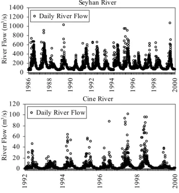
Seyhan River 0 200 400 600 800 1000 1200 1400 1986 1988 1990 1992 1994 1996 1998 2000 R ive r F low ( m 3/s

) _{Daily River Flow}

Fig. 6: River Flow Reco

Cine River 0 20 40 60 80 100 120 1992 1994 1996 1998 2000 R ive r F low ( m 3/s

) _{Daily River Flow}

g. 6: River Flow Records

Fig. 6. River flow records.

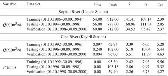
and rainfall data and other hydroclimatic variables at vari-ous time lags but in the present application, for the Seyhan river, it consists of combinations of antecedent daily river flow records, whereas for the Cine River, it consists of daily river flow and rainfall records are used in input layer. It is evi-dent that the training data sets should cover all the characters of the problem in order to get effective estimation. For the Seyhan River, the data set includes total 5114 daily river flow data and data set is divided into three subsets, training, test-ing and verification data set. The traintest-ing data set includes total 2922 daily river flow records measured at the time pe-riod 1986–1994 years, the testing data set consists of 1461 daily river data records measured between in 1994 and 1998 years. The verification data set consists of 731 daily river data records measured at the time 1998–2000 years. For the Cine River, total 2923 daily river flow and daily rainfall data was collected at the time period 1992 and 2000 years. The training set includes total 1464 data records at the time pe-riod 1992–1996 years, testing set consists of 730 data records measured between in 1996 and 1998 years. 731 daily river data records measured at the time 1998–2000 years was cho-sen for the verification of models. Figure 6 shows daily flow records of Seyhan River and Cine River. The minimum

value; xmin, maximum value; xmax, mean; ¯x, standard

devi-ation; sx, variation coefficient cvx, skewness coefficient; csx,

(7)

Table 1. The statistical parameters for data sets.

Variable Data Set x_min xmax x¯ sx csx

Seyhan River (Uctepe Station)

Q(t )(m3/s)

Training (01.10.1986–30.09.1994) 54.00 912.00 141.41 109.14 2.39 Testing (01.10.1994–30.09.1998) 56.00 778.00 160.96 111.34 2.05 Verification (01.10.1998–30.09.2000) 60.80 712.00 134.52 95.42 2.37

Cine River (Kayirli Station)

Q(t )(m3/s) Training (01.10.1992–30.09.1996) 0.097 62.94 3.39 6.05 5.28 Testing (01.10.1996–30.09.1998) 0.248 102.00 5.18 10.04 5.44 Verification (01.10.1998–30.09.2000) 0.094 96.00 5.51 11.39 4.63 P (mm) Training (01.10.1992–30.09.1996) 0.00 95.30 2.42 7.93 5.56 Testing (01.10.1996–30.09.1998) 0.00 103.15 2.86 9.97 5.32 Verification (01.10.1998–30.09.2000) 0.00 59.40 2.26 6.73 4.27

Table 2. Cross correlations between variables.

Seyhan River Q(t −1) Q(t −2) Q(t −3) Q(t −4) Q(t −5) Q(t −6) Q(t −7) Q(t ) 0.984 0.963 0.945 0.930 0.917 0.906 0.897 Cine River Q(t −1) Q(t −2) Q(t −3) P (t ) P (t −1) P (t −2) Q(t ) 0.97 0.95 0.93 0.45 0.40 0.38 6.2 Model structure

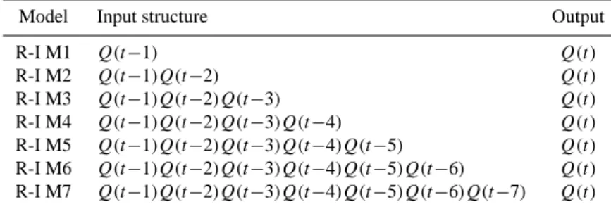
One of the most important steps in developing a satisfac-tory forecasting model is the selection of the input variables. Hence, cross- correlations between input and output vari-ables are calculated in order to apply the methods for model-ing (Table 2). Different combinations of the antecedent flows of river flow gauge station are used to construct the appro-priate input structure. The structures of models for Seyhan River and Cine River are shown in Tables 3 and 4, respec-tively.

Where Qt represents the River flow at time (t ),

Q(t −1), . . . Q(t−n) are the river flow respectively at times

(t−1). . . (t−n). Pt represents the rainfall at time (t ),

P (t −1), . . . P (t−n) are the rainfall respectively at times (t−1). . . (t−n). The training and testing experiments with ANFIS and ANN methods are carried out considering vari-ous input layer structures. The performances of the models both training and testing data are evaluated and compared ac-cording to Correlation Coefficient (CORR), Efficiency (E), Root Mean Square Error (RMSE), Mean Error in forecast-ing the maximum peak discharge value (%MERR) and the maximum percentage error (%MP).

CORR= N P t =1 (QD(t )−QD).(QY (t )−QY) s N P t =1 (QD(t )−QD)2.(QY (t )−QY)2 (17) E=E1−E2 E1 E1= N X t =1 (QD(t )−QD)2, E2= N X t =1 (QY(t )−QD(t ))2 (18) RMSE= " _N X t =1 (QD(t )−QY (t ))2 N #0.5 (19)

%MERR=(QYmax−QDmax

QDmax

).100 (20)

%MP=(QY−QD

QD

)max.100 (21)

where, QY is the forecasted river flow, QD is the field

ob-servation of river flow, QY is the average of the forecasted

(8)

Table 3. The structure of the models for forecasting of Seyhan river flow.

Model Input structure Output

R-I M1 Q(t −1) Q(t ) R-I M2 Q(t −1)Q(t −2) Q(t ) R-I M3 Q(t −1)Q(t −2)Q(t −3) Q(t ) R-I M4 Q(t −1)Q(t −2)Q(t −3)Q(t −4) Q(t ) R-I M5 Q(t −1)Q(t −2)Q(t −3)Q(t −4)Q(t −5) Q(t ) R-I M6 Q(t −1)Q(t −2)Q(t −3)Q(t −4)Q(t −5)Q(t −6) Q(t ) R-I M7 Q(t −1)Q(t −2)Q(t −3)Q(t −4)Q(t −5)Q(t −6)Q(t −7) Q(t )

Table 4. The structure of the models for forecasting of Cine river flow.

Model Input structure Output

R-II M1 P (t ) Q(t ) R-II M2 P (t )P (t −1) Q(t ) R-II M3 P (t )P (t −1)P (t −2) Q(t ) R-II M4 Q(t −1)P (t) Q(t ) R-II M5 Q(t −1)P (t)P (t −1) Q(t ) R-II M6 Q(t −1)P (t)P (t −1)P (t −2) Q(t ) R-II M7 Q(t −1)Q(t −2)P (t) Q(t ) R-II M8 Q(t −1)Q(t −2)P (t)P (t −1) Q(t ) R-II M9 Q(t −1)Q(t −2)P (t)P (t −1)P (t −2) Q(t ) R-II M10 Q(t −1)Q(t −2)Q(t −3)P (t) Q(t ) R-II M11 Q(t −1)Q(t −2)Q(t −3)P (t)P (t −1) Q(t ) R-II M12 Q(t −1)Q(t −2)Q(t −3)P (t)P (t −1)P (t −2) Q(t )

The correlation coefficient is a commonly used statistic and provides information on the strength of linear relationship between the observed and the computed values. The effi-ciency (E) is one of the widely employed statistics to evaluate model performance. An efficiency of 1 (E=1) corresponds to a perfect match of modeled discharge to the observed data. It should be noted that Nash-Sutcliffe efficiencies can also be used to quantitatively describe the accuracy of model out-puts other than discharge. This method can be used to de-scribe the predicative accuracy of other models as long as there is observed data to compare the model results. The values of CORR and E close to 1.0 indicate good model per-formance. RMSE evaluates the residual between measured and forecasted river flow. RMSE is a frequently-used mea-sure of the difference between values predicted by a model or an estimator and the values actually observed from the thing being modeled or estimated. These differences are also called residuals. Theoretically, if this criterion equals zero then model represents the perfect fit, which is not possible at all. The %MERR is the error in forecasting the maximum peak discharge value and it is useful in designing dams and bridges. The MP is an unbiased statistic for measuring the predictive capability of a model. It is clear that small %MP values indicate better model performance

6.2.1 ANFIS Model

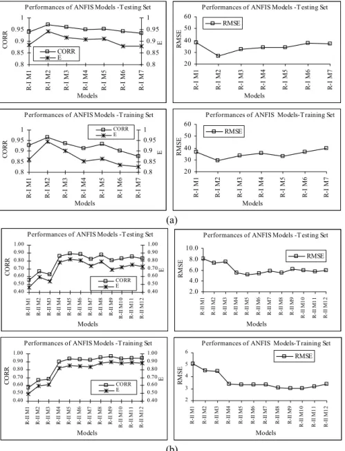
In this study firstly, the seven models having various input variables are trained and tested by ANFIS method and the performances of models for river flow forecasting models are compared and evaluated based on training and testing perfor-mances. The best fit model structure is determined according to criteria of performance evaluation. The performances of the ANFIS models for both stations are shown in Fig. 7.

As can be seen in Fig. 7, the ANFIS models are evaluated based on their performance in testing sets. The models have shown significant variations in the criteria of the performance evaluation given in Fig. 7. Firstly, for Seyhan River, it shows that the lowest value of the RMSE and the highest values of the E and CORR are R-I M2 ANFIS model. R-I M2 AN-FIS model, which consists of two antecedent flows in input, has shown the highest efficiency, correlation and the mini-mum RMSE and R-I M2 was selected as the best-fit model for modeling of Seyhan river flow in the Seyhan catchment. Secondly, comparing the performances of ANFIS model for Cine River, it is seen that R-II M5 ANFIS model, which has three input variables in input layer, has shown the best fit per-formance. The highest values of E and CORR criteria were obtained from R-II M5 ANFIS model. According to criteria,

(9)

Performances of ANFIS Models -T esting Set 0.8 0.85 0.9 0.95 1 R-I M 1 R-I M 2 R-I M 3 R-I M 4 R-I M 5 R-I M 6 R-I M 7 Models CO R R 0.8 0.85 0.9 0.95 1 E CORR E

Performances of ANFIS Models -T esting Set

20 30 40 50 60 R -I M 1 R -I M 2 R -I M 3 R -I M 4 R -I M 5 R -I M 6 R -I M 7 Models RM S E RMSE

Performances of ANFIS Models -T raining Set

0.8 0.85 0.9 0.95 1 R -I M 1 R -I M 2 R -I M 3 R -I M 4 R -I M 5 R -I M 6 R -I M 7 Models CO RR 0.8 0.85 0.9 0.95 1 E CORR E

Performances of ANFIS Models-T raining Set

20 30 40 50 60 R-I M 1 R-I M 2 R-I M 3 R-I M 4 R-I M 5 R-I M 6 R-I M 7 Models RM S E RMSE (a) Performances of ANFIS Models -T esting Set

0.40 0.50 0.60 0.70 0.80 0.90 1.00 R-II M 1 R-II M 2 R-II M 3 R-II M 4 R-II M 5 R-II M 6 R-II M 7 R-II M 8 R-II M 9 R-II M 1 0 R-II M 1 1 R-II M 1 2 Models CO R R 0.40 0.50 0.60 0.70 0.80 0.90 1.00 E CORR E

Performances of ANFIS Models -T esting Set

2.0 4.0 6.0 8.0 10.0 R-II M 1 R-II M 2 R-II M 3 R-II M 4 R-II M 5 R-II M 6 R-II M 7 R-II M 8 R-II M 9 R-II M 1 0 R-II M 1 1 R-II M 1 2 Models RM S E RMSE

Performances of ANFIS Models -T raining Set

0.40 0.50 0.60 0.70 0.80 0.90 1.00 R -II M 1 R -II M 2 R -II M 3 R -II M 4 R -II M 5 R -II M 6 R -II M 7 R -II M 8 R -II M 9 R -II M 1 0 R -II M 1 1 R -II M 1 2 Models CO RR 0.40 0.50 0.60 0.70 0.80 0.90 1.00 E CORR E

Performances of ANFIS Models-T raining Set

2 3 4 5 6 R-II M 1 R-II M 2 R-II M 3 R-II M 4 R-II M 5 R-II M 6 R-II M 7 R-II M 8 R-II M 9 R-II M 1 0 R-II M 1 1 R-II M 1 2 Models RM S E RMSE (b)

Fig. 7: Performances of ANFIS models, a) Seyhan River, b) Cine River)

Fig. 7. Performances of ANFIS models, (a) Seyhan River, (b) Cine River.

Table 5. The performance of ANFIS models.

Model Testing Data Set Training Data Set

RMSE E CORR RMSE E CORR

Seyhan River

R-I M2 ANFIS 26.95 0.941 0.970 29.43 0.945 0.964 Cine River

(10)

T esting Data Set

0 200 400 600 800 1000 1 366 731 1096 1461 Data Set (1994-1998) D a il y F lo w ( m 3/s ) R-I M2 ANFIS Observation

T esting Data Set- R-I M2 ANFIS

0 250 500 750 1000 0 250 500 750 1000 Observation Flow (m3/s) E st im at ed F low ( m 3 /s ) River Flow

T raining Data Set

0 200 400 600 800 1000 1 726 1451 2176 2901 Data Set (1986-1994) D ai ly F lo w ( m 3/s ) R-I M2 ANFIS Observation

T raining Data Set- R-I M2 ANFIS

0 250 500 750 1000 0 250 500 750 1000 Observation Flow (m3_/s) E st im a te d F low (m 3/s ) River Flow

(a)

T esting Data Set

0 30 60 90 120 1 365 729 Data Set (1996-1998) D a il y F low ( m 3/s ) R-II M5 ANFIS Observation

T esting Data Set- R-II M5 ANFIS

0 30 60 90 120 0 30 60 90 120 Observation Flow (m3_/s) E st im at ed F lo w ( m 3/s ) River Flow

T raining Data Set

0 20 40 60 80 1 726 1451 Data Set (1992-1996) D a il y F lo w ( m 3/s ) R-II M5 ANFIS Observation

T raining Data Set- R-II M5 ANFIS

0 20 40 60 80 0 20 40 60 80 Observation Flow (m3_/s) E st im at ed F low ( m 3/s ) River Flow

(b)

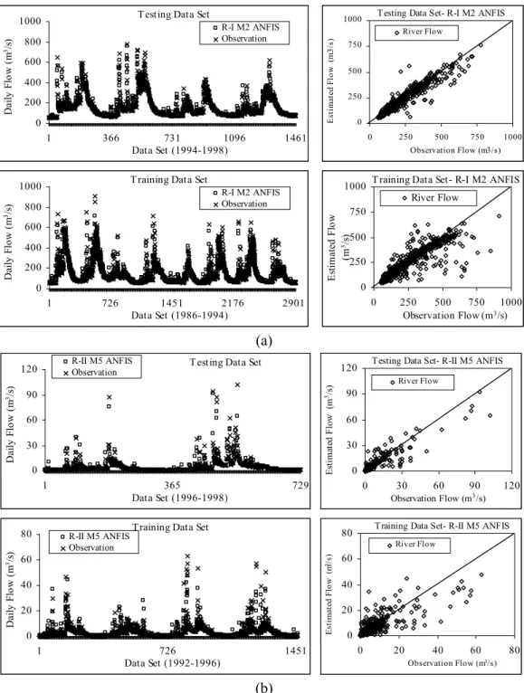
Fig. 8: The results of training and testing of models a) R-I M2 ANFIS b) R-II M5 ANFIS

Fig. 8. The results of training and testing of models (a) R-I M2 ANFIS (b) R-II M5 ANFIS.

R-II M5 ANFIS was selected as the best fit river flow fore-casting model for Cine River. The performances of the best fit ANFIS models for both stations are shown in Table 5.

It appears that the both ANFIS models generally are ac-curate and the values of RMSE are small enough, and cor-relation coefficients and efficiencies are very close to unity. The results of R-I M2 ANFIS model for Seyhan River and

R-I M5 ANFIS model for Cine River are compared with the observed flows in order to evaluate the performance of the training/testing of the model. Figure 8 shows the scatter di-agrams of the estimated values of the training/testing of R-I M2ANFIS and R-II M5 ANFIS models and observed values. The results of the ANFIS model demonstrate that the AN-FIS can be successfully applied to establish accurate and

(11)

reli-Performances of GRNN Models -T esting Set 0.40 0.50 0.60 0.70 0.80 0.90 1.00 R-II M 1 R-II M 2 R-II M 3 R-II M 4 R-II M 5 R-II M 6 R-II M 7 R-II M 8 R-II M 9 R-II M 1 0 R-II M 1 1 R-II M 1 2 Models CO R R 0.40 0.50 0.60 0.70 0.80 0.90 1.00 E CORR E

Performances of GRNN Models -T esting Set

4.0 6.0 8.0 10.0 R -II M 1 R -II M 2 R -II M 3 R -II M 4 R -II M 5 R -II M 6 R -II M 7 R -II M 8 R -II M 9 R-II M 1 0 R-II M 1 1 R-II M 1 2 Models RM S E RMSE

Performances of FFNN Models -T esting Set

0.40 0.50 0.60 0.70 0.80 0.90 1.00 R -II M 1 R -II M 2 R -II M 3 R -II M 4 R -II M 5 R -II M 6 R -II M 7 R -II M 8 R -II M 9 R -II M 1 0 R -II M 1 1 R -II M 1 2 Models CO RR 0.40 0.50 0.60 0.70 0.80 0.90 1.00 E CORR E

4.0 6.0 8.0 10.0 R -II M 1 R -II M 2 R -II M 3 R -II M 4 R -II M 5 R -II M 6 R -II M 7 R -II M 8 R -II M 9 R -II M 1 0 R -II M 1 1 R -II M 1 2 Models RM S E RMSE

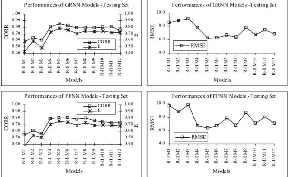
Fig. 9: The Performances of GRNN and FFNN models for Cine River

Fig. 9. The Performances of GRNN and FFNN models for Cine River.

able river flow forecasting models. In order to get a true and effective evaluation of the performance of ANFIS method, the models were also trained and tested by GRNN and FFNN methods.

6.2.2 ANN Models

In this study, secondly, the GRNN and FFNN methods are used for modeling of daily river flow. In the training and testing of ANN models, the same data set is used and per-formances of models are also evaluated and compared based on given above criteria. Figure 9 shows the performances of GRNN and FNNN models for Cine River. Moreover, Fig. 10 shows the performances of GRNN and FFNN models for Seyhan River.

Comparing the results of GRNN and FFNN models for Cine River given in Fig. 9, it said that the performances of the R-II M5 and R-II M8 models are near to each other and bet-ter than those of other models. The values of CORR and E of R-II M5 and R-II M8 models are higher than those of other models. Moreover, RMSE values of these models are also lower than those of other models. Although performances of R-II M5 and R-II M8 models are close to each other, results of R-II M5 models are better than R-II M8 models. As a result, R-II M5 GRNN and R-II M5 FFNN models were se-lected as the best fit forecasting models. The error backpra-gation algorithm and sigmoid activation function was used for the training and testing of FFNN model. The number of hidden neurons (5) in one hidden layer, the learning rate (0.05), the coefficient of momentum (0.7) and epochs (5000)

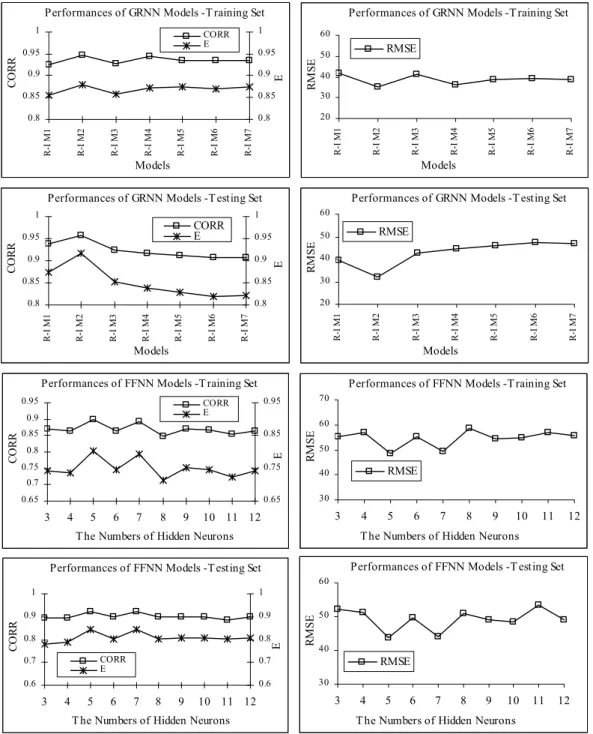
were selected by trial and error method during the training process. On the other hand, as can be seen in Fig. 10, the val-ues of the E and CORR of R-I M2 GRNN model for Seyhan River are higher than those of other models. In addition the value of RMSE of R-I M2 GRNN model is also lower than that of other models. As a result, R-I M2 GRNN model is se-lected as the best fit forecasting model according to criteria of performance evaluation. In order to get a true and effective evaluation, the best fit model structure having two input vari-ables has also been trained and tested by FFNN. The FFNN model having two input variables was trained and tested us-ing the same non-transformed data set. As can be seen in Fig. 10, the FNN model, which has five hidden neurons in hidden layer, has shown the best fit performance. The train-ing parameters of the FFNN model such as, the learntrain-ing rate (0.02), the coefficient of momentum (0.7) and epochs (2000) were selected by trial and error method during the training. The performances of forecasting models are given for both training and testing sets in Table 6 and Fig. 11.

Comparing the performances of R-I M2 GRNN and R-I M2 FFNN forecasting models for Seyhan River, it is seen that the value of the RMSE of the GRNN model is lower than FFNN model. In addition, the values of E and CORR of the R-I M2 GRNN model are also higher than R-I M2 FFNN model. For Cine River, it can be said that the performance of R-II M5 GRNN model is better than R-II M5 FFNN model according to criteria given in Table 5. It may be noted that a trial and error procedure has to be performed for FFNN mod-els to develop the best network structure, while such a proce-dure is not required in developing a GRNN model. The

(12)

re-M. Firat: Comparison of Artificial Intelligence Techniques for river flow forecasting 133

Performances of GRNN Models -T raining Set

0.8 0.85 0.9 0.95 1 R-I M 1 R-I M 2 R-I M 3 R-I M 4 R-I M 5 R-I M 6 R-I M 7 Models CO R R 0.8 0.85 0.9 0.95 1 E CORR E

Performances of GRNN Models -T raining Set

20 30 40 50 60 R-I M 1 R-I M 2 R-I M 3 R-I M 4 R-I M 5 R-I M 6 R-I M 7 Models RM S E RMSE

0.8 0.85 0.9 0.95 1 R-I M 1 R-I M 2 R-I M 3 R-I M 4 R-I M 5 R-I M 6 R-I M 7 Models CO R R 0.8 0.85 0.9 0.95 1 E CORR E

20 30 40 50 60 R-I M 1 R-I M 2 R-I M 3 R-I M 4 R-I M 5 R-I M 6 R-I M 7 Models RM S E RMSE

Performances of FFNN Models -T raining Set

0.65 0.7 0.75 0.8 0.85 0.9 0.95 3 4 5 6 7 8 9 10 11 12

T he Numbers of Hidden Neurons

CO R R 0.65 0.75 0.85 0.95 E CORR E

Performances of FFNN Models -T raining Set

30 40 50 60 70 3 4 5 6 7 8 9 10 11 12

RM

S

E

RMSE

0.6 0.7 0.8 0.9 1 3 4 5 6 7 8 9 10 11 12 T he Numbers of Hidden Neurons

CO RR 0.6 0.7 0.8 0.9 1 E CORR E

30 40 50 60

3 4 5 6 7 8 9 10 11 12

RM

S

E

RMSE

Fig. 10: The Performances of GRNN and FFNN models for Seyhan River

Fig. 10. The performances of GRNN and FFNN models for Seyhan River.

sults suggest that the GRNN method is superior to the FFNN method in the modeling and forecasting of the river flow. On the other hand, comparing the performances of ANFIS and ANN models for both stations, generally it is seen that the sults of ANFIS models are better than ANN models. As a re-sult, the results of training and testing of models demonstrate that ANFIS method is superior to ANN methods in forecast-ing of river flow. Moreover, it is said that ANFIS method can

be successfully applied for river flow forecasting according to performance criteria.

6.2.3 Autoregressive Model

In order to get more accurate and reliable evaluation and comparison the best fit input structures were used to forecast the daily river flow by using traditional forecasting method. For the Seyhan river, AR (2) model includes two river flow

(13)

T esting Data Set- R-I M2 GRNN 0 250 500 750 1000 0 250 500 750 1000 Observation Flow (m3/s) E st im a te d F lo w ( m 3 /s ) River Flow

T raining Data Set- R-I M2 GRNN

0 250 500 750 1000 0 250 500 750 1000

Observat ion Flow (m3/s)

E st im a te d F lo w ( m 3 /s ) River Flow

T esting Data Set- R-I M2 FFNN

0 250 500 750 1000 0 250 500 750 1000 Observation Flow (m3/s) E st im a te d F lo w ( m 3 /s ) River Flow

T raining Data Set- R-I M2 FFNN

0 250 500 750 1000 0 250 500 750 1000

Observat ion Flow (m3/s)

E st im a te d F lo w ( m 3 /s ) River Flow

(a)

T esting Data Set- R-II M5 GRNN

0 30 60 90 120 0 30 60 90 120 Observation Flow (m3/s) E st im a te d F low (m 3 /s ) River Flow

T raining Data Set- R-II M5 GRNN

T esting Data Set- R-II M5 FFNN

T raining Data Set - R-II M5 FFNN

(b)

Fig. 11: Results of training and testing of GRNN and FFNN models

a) Seyhan River, b) Cine River

(14)

Table 6. Comparison of performances of forecasting models.

Models Testing Data Set Training Data Set

RMSE E CORR RMSE E CORR

Seyhan River R-I M2 ANFIS 26.95 0.941 0.970 29.43 0.945 0.964 R-I M2 GRNN 32.076 0.917 0.952 42.520 0.848 0.921 R-I M2 FFNN 43.830 0.845 0.924 48.475 0.803 0.900 Cine River R-II M5 ANFIS 5.189 0.822 0.891 3.3084 0.856 0.940 R-II M5 GRNN 6.200 0.782 0.854 3.561 0.806 0.905 R-II M5 FFNN 6.347 0.751 0.804 3.878 0.765 0.847

Table 7. Comparison of verification performances of models.

Models Verification Data Set

%MERR %MP RMSE E CORR

Seyhan River R-I M2 ANFIS −9.12 69.96 33.972 0.873 0.935 R-I M2 GRNN 14.49 72.32 37.189 0.860 0.928 R-I M2 FFNN 15.31 77.48 43.595 0.808 0.899 R-I M2 AR(2) −11.90 72.27 39.344 0.823 0.914 Cine River R-II M5 ANFIS −10.39 74.26 6.322 0.817 0.894 R-II M5 GRNN −13.82 76.34 6.864 0.738 0.865 R-II M5 FFNN 14.21 78.54 7.551 0.717 0.826 ARX Model −13.95 77.06 6.990 0.741 0.854

variables at two previous time lags in input vector, whereas for the Cine River ARX model has one river flow at one pre-vious time lag and rainfall variables at the (t ) and (t−1) time lags in input. Once the estimates of the traditional time se-ries model coefficients have been obtained using the train-ing data set, the model can be validated by computtrain-ing the performance statistics during both training and testing data sets. The training and testing results of AR model for Sey-han River and ARX model Cine River are shown in Fig. 12.

6.2.4 Verification of forecasting models

The best fit ANFIS, GRNN, FFNN, AR and ARX models for both Seyhan River and Cine River are verified by verifica-tion data set. For Seyhan River, the verificaverifica-tion set includes totally 731 daily river flow values at the time period 1998– 2000 years. For Cine River, total 730 daily river flow and rainfall data records measured at the time period 1998–2000 years was used to verify the performance of forecasting mod-els. The verification performances of all methods are given in Table 7.

For both stations, comparing verification performances of ANFIS, GRNN, FFNN, AR and ARX models, the values of RMSE of ANFIS models are lower than those of GRNN, FFNN, AR and ARX model. On the other hand, the values of E and CORR of ANFIS model are also higher than those of GRNN, FFNN, AR and ARX models. In addition, the best fit values of %MERR and %MP criteria were obtained from ANFIS models. Comparison of the verification results of models for Seyhan River and Cine River are demonstrated in Figs. 13 and 14, respectively.

7 Conclusions

In this study, applicability and capability of Artificial Intel-ligence techniques, ANFIS and ANN, and AR methods for daily river forecasting was investigated. To illustrate the ca-pability of these approaches, Seyhan River and Cine River was chosen as a case study. Models having various input variables were trained and tested for both stations. The per-formances of the models and observations were compared

(15)

T esting Data Set- R-I M2 AR Model 0 250 500 750 1000 0 250 500 750 1000 Observation Flow (m3/s) E st im at ed F low ( m 3 /s ) River Flow

T raining Data Set- R-I M2 AR Model

0 250 500 750 1000 0 250 500 750 1000 Observat ion Flow (m3/s)

E st im at ed F low ( m 3 /s ) River Flow

(a)

Testing Data Set- ARX Model

0 30 60 90 120 0 30 60 90 120 Observation Flow (m3_/s) E st im at ed F lo w ( m 3/s ) River Flow

Training Data Set- ARX Model

0 20 40 60 80 0 20 40 60 80 Observation Flow (m3_/s) E st im at ed F low ( m 3/s ) River Flow

(b)

Figure 12: The training and testing results of auto regressive models a) Seyhan River, b)Cin

River

ş

Fig. 12. The training and testing results of auto regressive models (a) Seyhan River, (b) Cine River.

and evaluated based on their performance in training and test-ing sets. For the Seyhan River, R-I M2 ANFIS model havtest-ing two antecedent flow variables was selected as the best fit river forecasting model according to criteria of performance eval-uation. Moreover, for the Cine River, R-II M5 ANFIS model, which has one river flow at one previous time lag and rainfall variables at the (t ) and (t−1) time lags in input, has shown the best fit performance. The models were also trained and tested by GRNN, FFNN and Auto Regressive methods (AR method for Seyhan River and ARX method for Cine River) for the same set of data and results were reported to get more accurate and sensitive comparison. The results suggest that the ANFIS method is superior to the ANN and AR meth-ods in the modeling and forecasting of river flow. It is said that the results of training, testing and verification of models demonstrate that ANFIS method is superior to ANN methods in forecasting of river flow according to criteria.

Acknowledgements. The author is grateful for Editor and

Anony-mous Reviewers for their helpful and constructive comments on an earlier draft of this paper.

Edited by: E. Toth

References

Arena, C., Cannarozzo, M., and Mazzola, M. R.: Multi-year drought frequency analysis at multiple sites by operational hy-drology – A comparison of methods, Phys. Chem. Earth, 31, 1146–1163, 2006.

ASCE Task Committee.: Artificial neural networks in hydrology-II: Hydrologic applications, J. Hydrol. Eng., ASCE, 5(2), 124–137, 2000.

Box, G. E. P. and Jenkins, G.: Time Series Analysis, Forecasting and Control, Holden-Day, San Francisco, CA, 1970.

BuHamra, S., Smaoui, N., and Gabr, M.: The Box–Jenkins analysis and neural networks: prediction and time series modeling, Appl. Math. Model., 27, 805–815, 2003.

Celikoglu, H. B.: Application of radial basis function and gener-alized regression neural networks in non-linear utility function specification for travel mode choice modeling, Math. Comput. Model., 44, 640–658, 2006.

Celikoglu, H. B. and Cigizoglu, H. K.: Public transportation trip flow modeling with generalized regression neural Networks, Adv. Eng. Softw., 38, 71–79, 2007.

Chen, S. H., Lin, Y. H., Chang, L. C., and Chang, F. J.: The strat-egy of building a flood forecast model by neuro-fuzzy network, Hydrol. Process., 20, 1525–1540, 2006.

(16)

Verification Data Set

0 200 400 600 800 1000 1 366 731 Data Set (1998-2000) D a il y F lo w ( m 3/s ) R-I M2 GRNN Observation

Verification Data Set- R-I M2 GRNN

0 250 500 750 1000 0 250 500 750 1000 Observation Flow (m3/s) E st im at ed F lo w ( m 3/ s) River Flow

0 200 400 600 800 1000 1 366 731 Data Set (1998-2000) D ai ly F lo w ( m 3/s ) R-I M2 FFNN Observation

Verification Data Set- R-I M2 FFNN

0 250 500 750 1000 0 250 500 750 1000 Observation Flow (m3/s) E st im at ed F lo w ( m 3/ s) River Flow

Verification Dat a Set

0 200 400 600 800 1000 1 366 731 Data Set (1998-2000) D a il y F low ( m 3/s ) R-I M2 ANFIS Observation

Verification Data Set- R-I M2 ANFIS

0 250 500 750 1000 0 250 500 750 1000 Observation Flow (m3/s) E st im at ed F lo w ( m 3 /s ) River Flow

0 200 400 600 800 1000 1 366 731 Data Set (1998-2000) D ai ly F lo w ( m 3/s ) R-I M2 AR Observation

Verification Data Set- R-I M2 AR Model

Fig. 13: Comparison of the verification results of models for Seyhan River

Fig. 13. Comparison of the verification results of models for Seyhan River.

Chang, F. J. and Chang, Y. T.: Adaptive neuro-fuzzy inference sys-tem for prediction of water level in reservoir, Adv. Water Res., 29, 1–10, 2006.

Chang, F. J, Hu, H. F, and Chen, Y.C.: Counter propagation fuzzy– neural network for river flow reconstruction, Hydrol. Process., 15, 219–232, 2001.

Chang, F. J., Chang, L. C., and Huang, H. L.: Real-time recur-rent learning neural network for stream-flow forecasting, Hydrol. Process., 16, 2577–2588, 2002.

Cigizoglu, H. K.: Generalized regression neural network in monthly

flow forecasting, Civ. Eng. Environ. Syst., 22(2), 71–84, 2005. Cigizoglu, H. K. and Alp, M.: Generalized regression neural

net-work in modeling river sediment yield, Adv. Eng. Softw., 37, 63–68, 2006.

Dawson, C. W., Harpham, C., Wilby, R. L., and Chen, Y.: Evalua-tion of artificial neural network techniques for flow forecasting in the River Yangtze, China, Hydrol. Earth Syst. Sci., 6, 619–626, 2002,

http://www.hydrol-earth-syst-sci.net/6/619/2002/.

(17)

Us-Verification Set 0 20 40 60 80 100 1 366 Dat a Set (1998-2000) D ai ly F lo w ( m 3/s ) R-II M5 ANFIS Observation

Verification Set- R-II M5 ANFIS

T esting Data Set

0 20 40 60 80 100 1 366 Data Set (1998-2000) D ai ly F lo w ( m 3/s ) R-II M5 GRNN Observation

Testing Data Set- R-II M5 GRNN

0 25 50 75 100 0 25 50 75 100 Observation Flow (m3/s) E st im at ed F low ( m 3 /s ) River Flow Verification Set 0 20 40 60 80 100 1 366 Data Set (1998-2000) D ai ly F lo w ( m 3/s ) R-II M5 FFNN Observation

Verification Set- R-II M5 FFNN

Verificat ion Set

0 20 40 60 80 100 1 366 Dat a Set (1998-2000) D ai ly F low (m 3/s ) ARX Model Observation

Verification Set- ARX Model

0 25 50 75 100 0 25 50 75 100 Observation Flow (m3_/s) E st im at e d F lo w ( m 3/s ) River Flow

Fig. 14: Comparison of the verification results of models for Cine River

Fig. 14. Comparison of the verification results of models for Cine River.

ing Artificial Neural Networks, Phys, Chem. Earth (B), 26, 1–7, 2001.

Firat, M. and G¨ung¨or, M.: Estimation of the Suspended Concen-tration and Amount by using Artificial Neural Networks, IMO Technical Journal, 15(3), 3267–3282, 2004.

Firat, M. and G¨ung¨or, M.: River flow estimation using adaptive neuro fuzzy inference system, Math. Comput. Simulat., 75(3–4), 87–96, 2007.

Firat, M.: Watershed modeling by adaptive Neuro- fuzzy inference system approach. Doctor of Philosophy Thesis, Pamukkale

Uni-versity, Turkey, 2007 (in Turkish).

Jain, A. and Kumar, A. M.: Hybrid neural network models for hy-drologic time series forecasting, Appl. Soft Comput., 7, 585– 592, 2007.

Jang, J. S. R., Sun, C. T, and Mizutani, E.: Neuro-Fuzzy and Soft Computing, PrenticeHall, ISBN 0-13-261066-3, 607 s., United States of America, 1997.

Kim, B., Lee, D.W ., Parka, K. Y., Choi, S. R., and Choi, S.: Predic-tion of plasma etching using a randomized generalized regression neural network, Vacuum, 76, 37–43, 2004.

(18)

Kisi, ¨O.: Daily pan evaporation modelling using a model-fuzzy computing technique, J. Hydrol., 329(3–4), 636–646, 2006. Komornik, J., Komornikova, M., Mesiar, R., Sz¨okeova, D., and

Szolgay, J.: Comparison of forecasting performance of nonlin-ear models of hydrological time series, Phys. Chem. Earth., 31, 1127–1145, 2006.

Liong, S. Y., Lim, W. H, Kojiri, T., and Hori, T.: Advance Flood forecasting for Flood stricken Bangladesh with a fuzzy reasoning method, Hydrol. Process., 14, 431–448, 2000.

Mahabir, C., Hicks, F. E, and Fayek, A. R.: Application of fuzzy logic to the seasonal runoff, Hydrol. Process., 17, 3749–3762, 2000.

Mohammadi, K., Eslami, H. R., and Kahawita, R.: Parameter esti-mation of an ARMA model for river flow forecasting using goal programming, J. Hydrol., 331, 293–299, 2006.

Nagy, H. M., Watanabe, K., and Hirano, M.: Prediction of Sedi-ment Load concentration in Rivers using Artificial Neural Net-work Model, J. Hydr. Eng., 128, 588–595, 2002.

Nayak, P. C., Sudheer, K. P., and Ramasastri, K. S.: Fuzzy comput-ing based rainfall-runoff model for real time flood forecastcomput-ing, Hydrol. Process., 17, 3749–3762, 2004a.

Nayak, P. C., Sudheer, K. P., Rangan, D. M, Ramasastri, K. S.: A Neuro Fuzzy computing technique for modeling hydrological time series, J. Hydrol., 29, 52–66, 2004b.

Owen, J. S., Eccles, B. J., Choo, B. S., and Woodings, M. A.: The application of auto–regressive time series modeling for the time-frequency analysis of civil engineering structures, Eng. Struct., 23, 521–536, 2001.

Ramadhas, A. S., Jayaraja, S., Muraleedharan, C., and Padmaku-mar, K.: Artificial neural networks used for the prediction of the cetane number of biodiesel, Renew. Ener., 31, 2524–2533, 2006.

Sajikumar, N. and Thandaveswara, B.S.: A non-linear rainfall– runoff model using an artificial neural network, J. Hydrol., 216, 32–55, 1999.

Sudheer, K. P. and Jain, A.: Explaining the internal behaviour of artificial neural network river flow models, Hydrol. Process., 18, 833–844, 2004.

Tingsanchali, T. and Guatam, M. R.: Application of tank, NAM, ARMA and neural network models to flood forecasting, Hydrol. Process., 14, 2473–2487, 2000.

Thomas, H. A. and Fiering, M. B.: Mathematical synthesis of streamflow sequences for the analysis of river basin by simula-tion, in: Design of Water Resources Systems, edited by: Mass, A., Harvard University Press, Cambridge, MA, 459–493, 1962. Toth, E., Brath, A., and Montanari, A.: Comparison of short-term

rainfall prediction models for real-time flood forecasting, J. Hy-drol., 239, 132–147, 2000.

S¸en Z.: Fuzzy Logic and Foundation”, ISBN 9758509233, Bilge K¨ult¨ur Sanat Publisher, Istabul, 172 pp., 2001.

S¸en, Z. and Altunkaynak, A.: A comparative fuzzy logic approach to runoff coefficient and runoff estimation, Hydrol. Process., 20, 1993–2009, 2006.

Yevjevich, V.: Fluctuations of Wet and Dry Years. Part-I. Research Data Assembly and Mathematical Models, Hydrology Paper 1, Colorado State University, Fort Collins, CO, 1963.

Zadeh, L. A.: Fuzzy sets, Information and Control, 8(3), 338–353, 1965.

Zhang, G. P.: Time series forecasting using a hybrid ARIMA and neural network model, Neurocomputing, 50, 159–175, 2003.