HAL Id: insu-01659757
https://hal-insu.archives-ouvertes.fr/insu-01659757
Submitted on 17 Sep 2020
HAL is a multi-disciplinary open access
archive for the deposit and dissemination of
sci-entific research documents, whether they are
pub-lished or not. The documents may come from
teaching and research institutions in France or
abroad, or from public or private research centers.
L’archive ouverte pluridisciplinaire HAL, est
destinée au dépôt et à la diffusion de documents
scientifiques de niveau recherche, publiés ou non,
émanant des établissements d’enseignement et de
recherche français ou étrangers, des laboratoires
publics ou privés.
Segmentation of photospheric magnetic elements
corresponding to coronal features to understand the
EUV and UV irradiance variability
J. Zender, R. Kariyappa, G. Giono, M. Bergmann, V. Delouille, Luc Damé,
Jean-François Hochedez, S. T. Kumara
To cite this version:
J. Zender, R. Kariyappa, G. Giono, M. Bergmann, V. Delouille, et al.. Segmentation of photospheric
magnetic elements corresponding to coronal features to understand the EUV and UV irradiance
vari-ability. Astronomy and Astrophysics - A&A, EDP Sciences, 2017, 605, A41 (11p.).
�10.1051/0004-6361/201629924�. �insu-01659757�
A&A 605, A41 (2017) DOI:10.1051/0004-6361/201629924 c ESO 2017
Astronomy
&
Astrophysics
Segmentation of photospheric magnetic elements corresponding
to coronal features to understand the EUV
and UV irradiance variability
?
J. J. Zender
1, R. Kariyappa
2, G. Giono
3, M. Bergmann
4, V. Delouille
5, L. Damé
6, J.-F. Hochedez
6,5, and S. T. Kumara
71 European Space Research and Technology Center (ESTEC), 2200 AG Noordwijk, The Netherlands
e-mail: [email protected]
2 Department of Physics and R&D Division, Vemana Institute of Technology, 560034 Bangalore, India
3 Department of Space and Plasma Physics, School of Electrical Engineering, Royal Institute of Technology KTH, 10044 Stockholm,
Sweden
4 Julius-Maximilians-Universität Würzburg, Institut für Informatik, 97074 Würzburg, Germany 5 Royal Observatory of Belgium, Circular Avenue 3, 1180 Brussels, Belgium
6 LATMOS (Laboratoire Atmosphères, Milieux, Observations Spatiales), 11 boulevard d’Alembert, 78280 Guyancourt, France 7 Department of Physics, APS College of Engineering, 560082 Bangalore, India
Received 18 October 2016/ Accepted 27 May 2017
ABSTRACT
Context.The magnetic field plays a dominant role in the solar irradiance variability. Determining the contribution of various magnetic features to this variability is important in the context of heliospheric studies and Sun-Earth connection.
Aims.We studied the solar irradiance variability and its association with the underlying magnetic field for a period of five years (January 2011–January 2016). We used observations from the Large Yield Radiometer (LYRA), the Sun Watcher with Active Pixel System detector and Image Processing (SWAP) on board PROBA2, the Atmospheric Imaging Assembly (AIA), and the Helioseismic and Magnetic Imager (HMI) on board the Solar Dynamics Observatory (SDO).
Methods.The Spatial Possibilistic Clustering Algorithm (SPoCA) is applied to the extreme ultraviolet (EUV) observations obtained from the AIA to segregate coronal features by creating segmentation maps of active regions (ARs), coronal holes (CHs) and the quiet sun (QS). Further, these maps are applied to the full-disk SWAP intensity images and the full-disk (FD) HMI line-of-sight (LOS) magnetograms to isolate the SWAP coronal features and photospheric magnetic counterparts, respectively. We then computed full-disk and feature-wise averages of EUV intensity and line of sight (LOS) magnetic flux density over ARs/CHs/QS/FD. The variability in these quantities is compared with that of LYRA irradiance values.
Results.Variations in the quantities resulting from the segmentation, namely the integrated intensity and the total magnetic flux density of ARs/CHs/QS/FD regions, are compared with the LYRA irradiance variations. We find that the EUV intensity over ARs/CHs/QS/FD is well correlated with the underlying magnetic field. In addition, variations in the full-disk integrated intensity and magnetic flux density values are correlated with the LYRA irradiance variations.
Conclusions.Using the segmented coronal features observed in the EUV wavelengths as proxies to isolate the underlying magnetic structures is demonstrated in this study. Sophisticated feature identification and segmentation tools are important in providing more insights into the role of various magnetic features in both the short- and long-term changes in the solar irradiance.
Key words. Sun: magnetic fields – Sun: atmosphere – Sun: corona
1. Introduction
Solar magnetic fields are manifested as distinct features on the Sun because their presence cause changes in the radiative properties of the solar atmosphere. The features with high mag-netic fields are known as active regions. In the photosphere, active regions may include both dark sunspots with intense mag-netic fields and bright faculae with weaker fields, as reviewed in (Solanki 2003). Therefore the average photospheric intensity of an active region depends on its average magnetic flux in a com-plex way (e.g. Ortiz & Rast 2005). However, active region in-tensity at chromospheric and coronal heights generally increases monotonically with increasing magnetic flux. This is presumably
? The movie associated to Fig. 2 is available at http://www.aanda.org
because the presence of the magnetic fields causes non-radiative energy to be channeled into the outer atmospheric layers of the Sun (e.g.Klimchuk 2006;Ermolli et al. 2014).
At chromospheric heights the different levels of intensity and magnetic flux lead to a picture of plages, chromospheric network, and bright points as the classes of surface structures associated with measurable magnetic fields on the Sun (e.g.
Skumanich et al. 1975). Although variations in the proportions of these various structures on the Sun produce variability in its radiative output, the details of the relationship between mag-netic structure evolution and solar spectral irradiance variabil-ity is not routinely determined from full-disk magnetograms and intensity images. Even though the magnetic structure evolution and its influence on solar irradiance is not yet carried out on a fully automated basis, first results for the total solar irradi-ance (TSI) and ultraviolet (UV), visible, and infrared (IR) part
of the spectrum were made available in recent years (Yeo et al. 2014a,b;Wenzler et al. 2006). Investigations on the UV and the extreme UV (EUV) part of the spectrum has been provided byHaberreiter et al.(2014)
Direct comparison of Ca
ii
K images and magnetograms shows the strong association between plage and strong field regions (Babcock & Babcock 1955; Leighton 1959; Howard 1959). Stepanov & Petrova(1959) gave the first magnetic flux versus Caii
K intensity curves measured in calcium faculae (plages) with an electronic magnetograph. Their linear-linear scatter plots are fitted with a smooth, slightly non-linear curve.Skumanich et al.(1975) made similar observations in the quiet Sun and suggested a linear relation between the absolute value of the magnetic flux density and Ca
ii
K-line intensity.AfterErmolli et al.(2009) demonstrated that Ca
ii
K spec-troheliogram time series from several observatories can be com-bined for an intensity distribution analysis of bright features covering timescales longer than one solar cycle, Bertello et al.(2016) correlated the Ca
ii
K time series to the sunspot numbers. They found that the two time series match very well with yearly correlation coefficients higher than 0.92. In an overview paper,Ermolli et al.(2014) discuss several solar cycle indices from the photosphere, chromosphere, and several coronal altitudes, and their potential inter-relation.
Pevtsov et al.(2003) have compared the disk-integrated so-lar X-ray flux to the total unsigned magnetic flux. Using al-most 10 yr of soft X-ray data from Yohkoh and full-disk mag-netograms from Kitt Peak, they found the relationship was a power law with an index between 1.6 and 2.0. However, they found a linear relationship for discrete solar features (X-ray bright points and active regions) as for other active stars. The relationships between the radiative and magnetic-flux densi-ties for the Sun-as-a-star have been studied byPreminger et al.
(2010). We have not been able to find solar studies comparing full-disk chromospheric flux to full-disk photospheric magnetic flux.Livingston et al.(2007) discussed the spectrum variability of the Sun-as-a-star and its correlation with the sunspot number.
Schrijver & Harvey (1989) and Harvey & White (1999) found that average Ca
ii
K-line flux density is proportional to the av-erage magnetic-flux density to the power 0.6, when averaging over non-sunspot chromospheric regions. Ortiz & Rast (2005) obtained a similar result when comparing Caii
K-line intensity with magnetic-flux density for image sections near the disk cen-tre. Also, Schrijver(1983) showed that the average solar coro-nal X-ray flux depends on the average chromospheric flux to the power ≈1.6.For more than three decades, the total solar irradiance (TSI) has been monitored from several radiometers from space (e.g.
Foukal & Lean 1988; Fröhlich et al. 1995; Kariyappa & Pap 1996; Rottman et al. 2006). Recent space instrumentation and improved understanding of instrument internal stray light con-tributions (Schmutz et al. 2013) has led to more accurate val-ues for the TSI and derived parameters (e.g.Kopp & Lean 2011;
Prša et al. 2016). It was observed that the solar energy flux changes over a solar cycle. It has been shown that the solar cycle irradiance variations are attributed to the changes in total bright-ness and area of the magnetic elements (Foukal & Lean 1988;
Kariyappa & Pap 1996; Worden et al. 1998; Kariyappa 2000,
2008; Veselovsky et al. 2001; Kumara et al. 2012; Yeo et al. 2014b) whereas the short-term irradiance variations are directly associated with active regions as they evolve and move across the solar disk (Lean 1987). To understand and clarify the di ffer-ence between the observed and modelled irradiance variability, know the underlying physical mechanisms of solar irradiance
variability, and determine the role of various coronal features and corresponding photospheric magnetic features in the EUV and UV irradiance, a detailed and accurate image analysis of spatially resolved observations of the intensity images and mag-netograms is required. To achieve this task, a successful segmen-tation of the solar features is necessary. The image segmensegmen-tation is an important tool in the reconstruction of solar spectral ir-radiance (SSI) in the line of the semi-empirical reconstruction approaches (Fontenla et al. 2009; Haberreiter 2011; Ball et al. 2011;Haberreiter et al. 2014;Fontenla et al. 2017).
Our objective in this study is the practical conversion of solar intensity and magnetic field images into physically interpretable quantities describing the solar magnetic cycle and its conse-quences on the radiative output of the Sun. We have used the Spatial Possibilistic Clustering Algorithm (SPoCA;Barra et al. 2008,2009;Verbeeck et al. 2014;Kumara et al. 2014), which is an image segmentation algorithm that allows the separation of solar intensity images and magnetograms into three character-istic structures on the Sun: active regions (ARs), coronal holes (CHs), and quiet sun (QS) (Kumara et al. 2014). Understanding the EUV and UV irradiance variability from spatially resolved intensity and magnetic field observations is an important issue in space weather and climate applications.
2. Observations and analysis
2.1. Observations
We used data from the Atmospheric Imaging Assembly (AIA;
Boerner et al. 2012) and Helioseismic and Magnetic Imager (HMI; Hoeksema et al. 2014) instruments on board the So-lar Dynamics Observatory (SDO; Pesnell et al. 2012) and the Large Yield Radiometer (LYRA; Hochedez et al. 2006;
Dominique et al. 2013) and the Sun Watcher with Active Pixel System detector and Image Processing telescope (SWAP;
Berghmans et al. 2006; Seaton et al. 2013), both on board the PROBA2 spacecraft. We have considered Level 1.5 AIA (171 Å, 193 Å) and Level 1 SWAP (174 Å) EUV images and HMI Level 1.5, full-disk line-of-sight (LOS) magnetograms. The SWAP and AIA images are corrected for dark currents, are flat-field corrected, bad pixels are removed, and the images are ro-tated such that the solar north is at the top. The SWAP imager ex-periences a detector degradation of less than 2% per year (private communication with the SWAP Principal Investigator), which may result in the increase of dark currents. These effects are also corrected for in the calibrated data. The data from the AIA im-ager was further cross-calibrated to the EVE calibration rocket under flight, which resulted in a good agreement of both. Fur-ther calibration rocket flights will allow an update of the AIA instrument spectral calibration curve (Boerner et al. 2012). The HMI LOS magnetograms are fully corrected for detector, op-tics, and degradation effects; see Couvidat et al. (2016) for a full description. The level 3 data of the aluminium filter chan-nel of the Large Yield Radiometer (LYRA) was used to compare against the solar irradiance over the full time period. The LYRA time series are fully radiometrically calibrated and then averaged over one minute. The detector is responsive to wavelengths from 17 nm−80 nm plus a contribution below 5 nm, including the strong He
ii
at 30.4 nm (Dominique et al. 2013).2.2. Analysis
In our previous paper, Kumara et al.(2014), we described the details of all the instruments, calibration of data, degradation
of instruments, and the SPoCA. We also explained the obser-vational details and procedure applied to segment the coro-nal features (ARs/CHs/QS/FD) for the period January 2011 to December 2012. In this paper we used the segmented maps of ARs/CHs/QS/FD from the previous analysis for 2 yr (2011 and 2012) and extended similar analysis up to January 2016. The time series are created by the following steps:
– Data selection;
– Segmentation of EUV images; – Creation of AR/CH/QS maps;
– Extending the AR maps into extended active regions (eAR) maps;
– Applying these maps on all EUV channels and HMI magnetograms;
– Creation of time series for eAR/CH/QS for each EUV chan-nel and HMI magnetogram by integration over all pixels of a coronal feature.
The maps have been projected/overlaid onto the HMI full-disk LOS magnetograms to segment the photospheric magnetic fea-tures corresponding to coronal ARs/CHs/QS regions for the pe-riod of five years. Our analysis also includes the integrated in-tensity over the full disk (FD).
For the period of five years, starting from January 1, 2011, we selected the HMI magnetograms that are nearest in time to the available AIA segmentation maps. In order to study the long-term variations, we selected six equally distributed images per day. The segmentation maps are arrays with the same dimen-sion as the input images; these are 4k × 4k arrays in the case of AIA and 1k × 1k arrays in the case of SWAP. In order to apply the segmentation maps on HMI magnetograms, it is necessary to first match the image scale between the different instruments. To achieve this, we rescaled the SPoCA maps by taking the ra-tio of the solar disk radii from AIA and HMI observara-tions as a scaling parameter. Furthermore, we aligned the AIA maps to achieve spatial alignment between the SWAP maps, AIA maps, and HMI magnetograms. The full resolution AIA segmentation maps were used on AIA images to compute the integrated inten-sity values over ARs/CHs/QS/FD. We then rebinned these seg-mentation maps and the AIA and SWAP images to align with HMI magnetograms. The pixels of the map can have either zero or non-zero values. Non-zero values correspond to the pixels lo-cated in an ARmap or CHmap. Since maps and images have the same size, they share the same coordinate system. For exam-ple, all non-zero pixels in an ARmap have the same coordinates as all the pixels inside active regions in the corresponding AIA image. It is easy to extract these coordinates with the WHERE command in IDL. Therefore we can obtain the coordinates of all pixels inside ARs and CHs using ARmaps and CHmaps.
After applying the ARmaps onto the LOS magnetograms, each individual active region is further expanded into its neigh-bourhood pixels. By careful visual inspection of many active region areas, we found that this extension would improve the overall segmentation. For coronal hole regions, a further adapta-tion of the segmented region was found to be of marginal value. The effects due to the different acquisition time between the in-dividual channels and observations of magnetograms and EUV images at different altitudes are not considered in our analysis. The extended magnetic regions are indicated as extended active regions, eAR, in the following section.
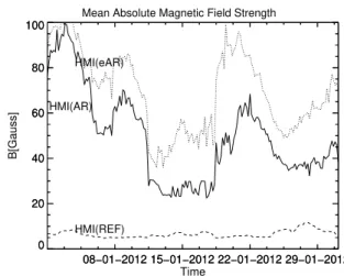
The mean value of the magnetic flux within a month of ARHMIis, for example for January 2012, 49 Gauss and the
stan-dard deviation is 20 Gauss. The monthly mean and stanstan-dard deviation of the eARHMI is 70 and 19 Gauss, respectively. For
08−01−2012 15−01−2012 22−01−2012 29−01−2012 0 20 40 60 80 100 08−01−2012 15−01−2012 22−01−2012 29−01−2012 Time 0 20 40 60 80 100 B[Gauss] HMI(AR) HMI(eAR) HMI(REF)
Mean Absolute Magnetic Field Strength
Fig. 1.Mean values of the absolute magnetic field of the ARs, eARs, and a reference region for January 2012. The solid line represents the mean value obtained for each image of the absolute values of the mag-netic field within an active region, the dotted line represents the cor-responding values of the extended active region, and the dashed line represents the values of a reference region.
comparison, we selected a reference region in the centre of the solar disk (indicated as REF in Fig.1). The region is the same size, i.e. the same amount of pixels, but does not include any ac-tive region nor coronal hole pixels. The region has a mean value of 6.5 and a standard deviation of 1.5 Gauss. Figure1shows the evolution of the daily mean values described above for the month of January 2012.
Our algorithm extends the ARHMIinto an eARHMIin the
fol-lowing way: let eARHMIbe ARHMI. For each adjacent pixel
out-side of eARHMI check if its value is above a threshold T and
expand eARHMIwith the selected pixel. The selection is repeated
until all adjacent pixels are below the threshold T . The eARHMI
is thus always larger or equal than the original projection ARHMI.
The threshold T was set to 35 Gauss, that is larger than the monthly mean value for the QS region (19 Gauss). The eARHMI
cover typically 20% more pixels than ARHMI, as can be seen
from Fig.1. We did not find a large correlation value between the mean absolute magnetic field values and the area increase between the ARHMIand the eARHMI. The Spearman rank coe
ffi-cient for this correlation is 0.55 for all data from 2012.
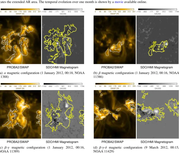
An illustration of SWAP and HMI maps is shown in Fig.2. With these coordinates, we can easily extract the pixel values of the ARs and CHs. In the left panel we show the SWAP 17.4 nm segmented ARs/CHs/QS/FD map. The right panel is the segmented map overlaid on the HMI magnetogram show-ing the eARs/ARs/CHs/QS/FD. features. In Fig.3, several cases for the extension algorithm are mapped, covering four exam-ples of the most common active regions classes, as defined byJaeggli & Norton(2016). The algorithm works satisfactorily for examples of active region classes α, β, β − γ, and β − γ − δ classes, as plotted in the individual sub-panels. Especially, in the case of complex active regions, i.e. the β − γ − δ case, the eAR is covering the increased magnetic activities. As these classes rep-resent more than 90% of the active regions (Jaeggli & Norton 2016), we assume that our mapping algorithm works satisfac-torily; see one-month movie attached to Fig .2. Variations in the quantities resulting from the segmentation, such as the integrated intensity and photospheric magnetic flux density of the coronal features and the full-disk observations, are compared with those of the LYRA irradiance and sunspot numbers. To allow a sta-tistical view on the analysis, a regression analysis is performed
(a) Proba2/SWAP 17.4 nm and SDO/HMI LOS magnetogram
Fig. 2. Left panel: segmentation maps resulting from the SPoCA algorithm applied on SWAP 17.4 nm image. The solid grey line indicates the segmented AR. The dotted grey line indicates the segmented CH. Right panel: photospheric magnetic features are identified in the HMI magnetogram using the SPoCA segmentation maps. The grey lines indicate the segmented features projected onto the magnetogram. The yellow line indicates the extended AR area. The temporal evolution over one month is shown by amovieavailable online.
0 45 89 134 178 223 268 312 357 SWAP DN
−1153 −662 −171 321 812 1303 1794 GAUSS
PROBA2/SWAP SDO/HMI Magnetogram
(a) α magnetic configuration (1 January 2012, 00:18, NOAA 11388)
0 45 89 134 178 223 268 312 357 SWAP DN
−1153 −662 −171 321 812 1303 1794 GAUSS
PROBA2/SWAP SDO/HMI Magnetogram
(b) β magnetic configuration (1 January 2012, 00:16, NOAA 11386)
0 45 89 134 178 223 268 312 357 SWAP DN
−1153 −662 −171 321 812 1303 1794 GAUSS
PROBA2/SWAP SDO/HMI Magnetogram
(c) β-γ magnetic configuration (1 January 2012, 00:16, NOAA 11389)
0 44 89 133 178 222 266 311 355 SWAP DN
−1598 −1032 −465 101 668 1234 1801 GAUSS
PROBA2/SWAP SDO/HMI Magnetogram
(d) β-γ-δ magnetic configuration (9 March 2012, 00:15, NOAA 11429)
Fig. 3.Left panels: coronal active region identified with the SPoCA segmentation maps for different magnetic configurations (grey lines). Right panels: photospheric magnetic features identified by the extended active region maps (yellow lines).
0.0 6.2 12.5 18.8 25.0 31.2 37.5 43.8 50.0 SWAP DN
−30 −20 −10 0 10 20 30
GAUSS
PROBA2/SWAP SDO/HMI Magnetogram
(a) 21 January 2012, 03:58, CH region
0.0 6.2 12.5 18.8 25.0 31.2 37.5 43.8 50.0 SWAP DN
−30 −20 −10 0 10 20 30
GAUSS
PROBA2/SWAP SDO/HMI Magnetogram
(b) 3 January 2012, 11:58, CH region Fig. 4.Coronal hole segmentation map examples overlaid onto the SWAP images (left) and the photospheric magnetic images (right).
by computing a linear fit y = a + bx for all parameters. The confidence interval for the offset a and the slope b is computed, along with the Spearman rank correlation coefficients and its 1σ uncertainty, as detailed inTamhane & Dunlop(2000).
3. Results
The segmented maps derived using the SPoCA algorithm from AIA (17.1 nm, 19.3 nm) images for the period of five years (Jan-uary 2011 to Jan(Jan-uary 2016) were applied to HMI full-disk LOS magnetograms. The SPoCA derived active region maps were ex-tended to all adjacent pixels with a magnetic flux of higher than 35 Gauss before the maps were applied to the HMI images. We computed the integrated magnetic flux density of the full-disk and eARs/CHs/QS/FD features from the segmented magnetic maps. We then compared these quantities with the SWAP seg-mented features, the daily-averaged SSI as observed with the LYRA aluminium channel (observed Sun as a star), and to the sunspot numbers. This comparison includes the calculation of the Spearman rank coefficient between all the observables.
3.1. Integrated intensity and absolute magnetic flux density variations of the segmented coronal features
In Fig.5we plot the time series of total absolute magnetic flux density of each of the coronal features (eARs, CHs, and QS) and full-disk absolute magnetic flux density from the SDO/HMI magnetograms. The LYRA aluminium channel irradiance for the five years is shown in the lower left panel. For comparison, we plotted the sunspot number for the same period in the right bot-tom panel. Further, Fig.6show the time series of feature-wise integrated intensity, the full-disk intensities obtained from the SWAP segmented maps, respectively, and the sunspot numbers for the corresponding period for comparison. Table 1 presents the mean, minimum, maximum, and standard deviation of the integrated intensity of ARs, CHs, QS, and the full disk de-rived from AIA images, the integrated magnetic flux densities of eARs, CHs, QS, and the full disk derived from HMI mag-netograms, and LYRA aluminium channel irradiance measure-ments for a five-year period.
It can be seen from the figures and Table1that the total mag-netic flux density of active regions is larger than that of the coro-nal holes, but smaller than the flux of the quiet sun. The area cov-ered by the quiet sun (QS) regions is larger than ARs and CHs,
hence the total absolute magnetic flux density is larger than that of ARs. Table1also lists the mean of the expected noise level for each segmented region of the magnetogram data. The noise level is computed as the product of the number of pixels and the detector shot noise, 5 Gauss, as specified inHoeksema et al.
(2014).
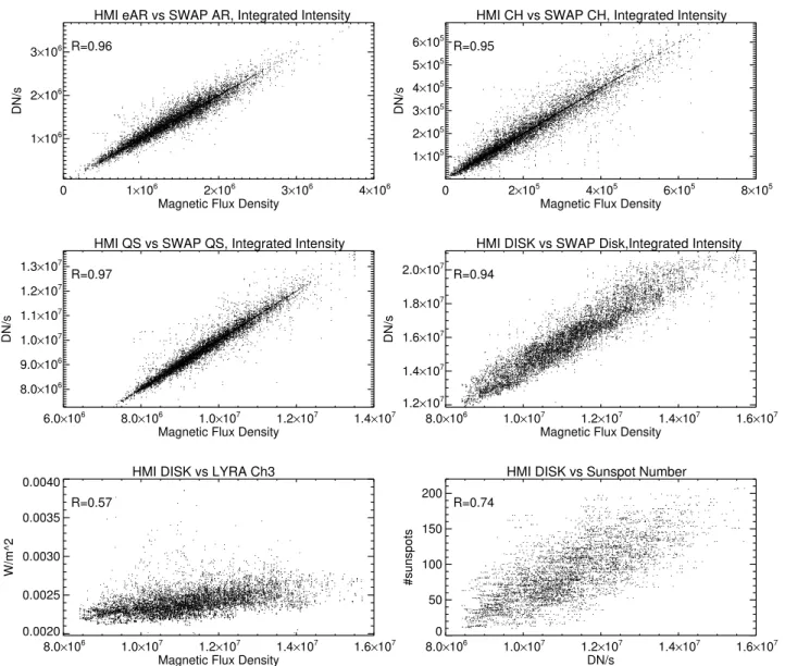
Figure 7 represent the scatter plots of integrated intensi-ties over SWAP coronal features against the respective HMI integrated absolute magnetic flux density. The bottom panels represent LYRA aluminium channel irradiance and the sunspot number versus the HMI full-disk average flux density. These scatter plots show that the ARs, CHs, QS, and FD intensities have good correlation with the corresponding absolute magnetic flux density.
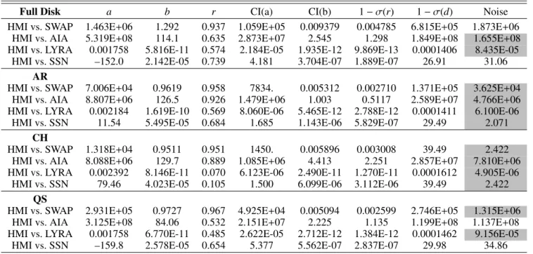
Table2gives a statistical analysis of all analysed time series. A linear regression analysis, y = a + bx, results in the offset a and slope b for a best mean-square linear fit. Further, the Spear-man correlation coefficients between HMI, AIA 17.1 m, SWAP 17.4 nm, and the LYRA aluminium channe, for all segmented features (ARs/CHs/QS) and the total integrated full-disk inten-sity (FD), are given. The second and third column in Table2list the linear fitting parameters a, b, and the Spearman correlation coefficient r, respectively. The next three columns list the 95% confidence intervals, thus the 1σ value, of these fitting parame-ters: Col. 5 lists the 95% confidence interval of the parameter a, Col. 6 the 95% confidence interval of the parameter b, and Col. 7 the 95% confidence interval of the correlation parameter r itself. The 1σ value of the difference d between the original data and fitted data, for example for the full-disk
d= FDSWAP− (a+ b ∗ FDHMI),
is listed in Col. 8. The last column represents the expected noise level n and is computed, for example for the full-disk value, as follows:
n= FDSWAP− (a+ b ∗ (FDHMI+ N(FDHMI)))
where N(FDHMI) is the number of pixels of the solar disk
multi-plied by the expected noise value (5 Gauss).
The correlation coefficients listed in Table2, Col. 4, indi-cate a very good relationship between all the SWAP and HMI time series. Noise levels, as listed in the last column in Table2, that are smaller than the 1σ value of the difference between the original and fitted data give us confidence in the significance of the calculated correlation coefficients. This is the case for most
HMI eAR absolute magnetic flux density
01/2011 01/2012 01/2013 01/2014 01/2015 01/2016 1×10⁶
2×10⁶
3×10⁶
HMI eAR INT (DN)
HMI CH absolute magnetic flux density
01/2011 01/2012 01/2013 01/2014 01/2015 01/2016 0 1×10⁵ 2×10⁵ 3×10⁵ 4×10⁵ 5×10⁵ 6×10⁵ HMI CH INT (DN)
HMI QS absolute magnetic flux density
01/2011 01/2012 01/2013 01/2014 01/2015 01/2016 8.0×10⁶ 9.0×10⁶ 1.0×10⁷ 1.1×10⁷ 1.2×10⁷ 1.3×10⁷ HMI QS INT (DN)
HMI FULL DISK averaged magnetic flux density
01/2011 01/2012 01/2013 01/2014 01/2015 01/2016 1.0×10⁷ 1.2×10⁷ 1.4×10⁷ HMI FD INT (DN) LYRA Irradiance 01/2011 01/2012 01/2013 01/2014 01/2015 01/2016 Time 0.0020 0.0025 0.0030 0.0035 0.0040 LyCH3 [W/m2]
Daily Sunspot Number
01/2011 01/2012 01/2013 01/2014 01/2015 01/2016 Time 50 100 150 200 #sunspots
Fig. 5.The time series of total magnetic flux density of eARs, CHs, QS, and full-disk obtained from the HMI magnetograms. The lower left panel shows the time series of LYRA aluminium channel irradiance observations and the lower right panel shows the daily sunspot number variations for comparison. All the quantities are plotted for the period of five years starting from 1 January 2011.
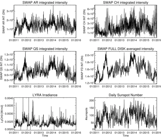
SWAP AR integrated intensity
01/2011 01/2012 01/2013 01/2014 01/2015 01/2016 1×10⁶
2×10⁶
3×10⁶
SWAP AR INT (DN)
SWAP CH integrated intensity
01/2011 01/2012 01/2013 01/2014 01/2015 01/2016 1×10⁵ 2×10⁵ 3×10⁵ 4×10⁵ 5×10⁵ 6×10⁵ SWAP CH INT (DN)
SWAP QS integrated intensity
01/2011 01/2012 01/2013 01/2014 01/2015 01/2016 8.0×10⁶ 9.0×10⁶ 1.0×10⁷ 1.1×10⁷ 1.2×10⁷ 1.3×10⁷ SWAP QS INT (DN)
SWAP FULL DISK averaged intensity
01/2011 01/2012 01/2013 01/2014 01/2015 01/2016 1.2×10⁷ 1.4×10⁷ 1.6×10⁷ 1.8×10⁷ 2.0×10⁷ SWAP FD INT (DN) LYRA Irradiance 01/2011 01/2012 01/2013 01/2014 01/2015 01/2016 Time 0.0020 0.0025 0.0030 0.0035 0.0040 LyCH3 [W/m2]
Daily Sunspot Number
01/2011 01/2012 01/2013 01/2014 01/2015 01/2016 Time 0 50 100 150 200 #sunspots
Table 1. Mean, minimum, maximum, and standard deviation of the time series for the five-year period on the integrated magnetic field of HMI, the integrated intensity of AIA and SWAP for ARs/CHs/QS/FD, and the LYRA aluminium channel irradiance observations.
AR CH QS FD LYRA AL
DN W m−2
For AIA: 1 Jan. 2011–1 Feb. 2016
Mean 1.744E+08 3.371E+07 1.133E+09 1.809E+09 2.386E-03
Min 9.859E+06 9.573E+05 7.576E+08 1.284E+09 1.000E-03
Max 4.683E+08 3.291E+08 1.750E+09 2.651E+09 4.000E-03
Stddev 7.104E+07 3.155E+07 1.446E+08 2.309E+08 2.047E-04
For HMI magnetograms: 1 Jan. 2011–1 Feb. 2016
Mean 1.301E+06 1.994E+05 9.467E+06 1.095E+07
Min 6.128E+02 3.052E-06 6.140E+06 6.638E+06
Max 3.679E+06 6.858E+05 1.351E+07 1.570E+07
Stddev 5.340E+05 1.231E+05 1.054E+06 1.486E+06
Noise 3.769E+04 6.021E+04 1.352E+06 1.450E+06
For SWAP magnetograms: 1 Jan. 2011–1 Feb. 2016
Mean 1.317E+06 2.018E+05 9.495E+06 1.557E+07
Min 4.442E+04 6.864E+02 6.894E+06 1.061E+07
Max 3.679E+06 6.858E+05 1.364E+07 2.113E+07
Stddev 5.359E+05 1.234E+05 1.064E+06 2.083E+06
Table 2. Regression statistics of all analysed time series.
Full Disk a b r CI(a) CI(b) 1 − σ(r) 1 − σ(d) Noise
HMI vs. SWAP 1.463E+06 1.292 0.937 1.059E+05 0.009379 0.004785 6.815E+05 1.873E+06
HMI vs. AIA 5.319E+08 114.1 0.635 2.873E+07 2.545 1.298 1.849E+08 1.655E+08
HMI vs. LYRA 0.001758 5.816E-11 0.574 2.184E-05 1.935E-12 9.869E-13 0.0001406 8.435E-05
HMI vs. SSN –152.0 2.142E-05 0.739 4.181 3.704E-07 1.889E-07 26.91 31.06
AR
HMI vs. SWAP 7.006E+04 0.9619 0.958 7834. 0.005312 0.002710 1.371E+05 3.625E+04
HMI vs. AIA 8.807E+06 126.5 0.926 1.479E+06 1.003 0.5117 2.589E+07 4.766E+06
HMI vs. LYRA 0.002184 1.619E-10 0.569 8.060E-06 5.465E-12 2.788E-12 0.0001411 6.100E-06
HMI vs. SSN 11.54 5.495E-05 0.684 1.685 1.143E-06 5.829E-07 29.49 2.071
CH
HMI vs. SWAP 1.318E+04 0.9511 0.951 1450. 0.005896 0.003008 39.49 2.422
HMI vs. AIA 8.088E+06 129.7 0.889 1.085E+06 4.413 2.251 2.857E+07 7.810E+06
HMI vs. LYRA 0.002392 8.146E-11 0.070 6.123E-06 2.490E-11 1.270E-11 0.0001612 4.905E-06
HMI vs. SSN 79.46 4.023E-05 0.105 1.500 6.099E-06 3.112E-06 39.49 2.422
QS
HMI vs. SWAP 2.931E+05 0.9727 0.967 4.925E+04 0.005094 0.002599 2.746E+05 1.315E+06
HMI vs. AIA 3.125E+08 84.06 0.532 2.151E+07 2.225 1.135 1.199E+08 1.137E+08
HMI vs. LYRA 0.001758 6.770E-11 0.485 2.622E-05 2.712E-12 1.384E-12 0.0001462 9.156E-05
HMI vs. SSN –159.8 2.578E-05 0.654 5.377 5.562E-07 2.837E-07 29.98 34.86
of the correlations and indicated by the greyed cells in the last column of Table2.
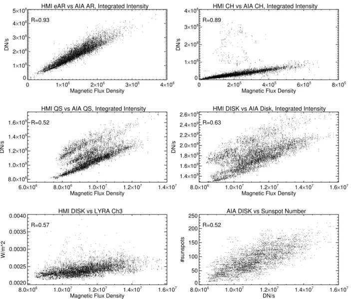
The correlation coefficients between the corresponding HMI and AIA features are high and they are particularly significant for AR and CH, but a low correlation was found for the full-disk and QS regions. Figure 8 show the scatter plots of integrated intensities over the AIA coronal features against the respective HMI magnetic flux density. Table3contains the yearly correla-tion coefficients and a good and significant correlation between the AIA features and the magnetic flux densities was identified.
As discussed in Raftery et al. (2013), the AIA 17.1 nm and the SWAP 17.4 nm bandpasses are considerably di ffer-ent. Whereas the AIA 17.1 nm bandpass has a sharp response
peak at 17.1 nm, the SWAP response is flat between 17.0 nm and 17.7 nm. These observations and the different spectral in-strument response characteristics might indicate that the AIA 17.1 nm channel shows either a long-term drift, as noted earlier inKumara et al.(2012) andBenMoussa et al.(2013), or that the QS intensity at 17.1 nm is decreasing in time. A more detailed study on these observations is needed.
3.2. Full-disk magnetic field and intensity variations in comparison with LYRA EUV and UV irradiance As observed through the scatter plots (Fig. 5) the full-disk in-tensity of SWAP is correlated well with their corresponding
0 1×10⁶ 2×10⁶ 3×10⁶ 4×10⁶
Magnetic Flux Density 1×10⁶
2×10⁶
3×10⁶
DN/s
R=0.96
HMI eAR vs SWAP AR, Integrated Intensity
0 2×10⁵ 4×10⁵ 6×10⁵ 8×10⁵
Magnetic Flux Density 1×10⁵ 2×10⁵ 3×10⁵ 4×10⁵ 5×10⁵ 6×10⁵ DN/s R=0.95
HMI CH vs SWAP CH, Integrated Intensity
6.0×10⁶ 8.0×10⁶ 1.0×10⁷ 1.2×10⁷ 1.4×10⁷
Magnetic Flux Density 8.0×10⁶ 9.0×10⁶ 1.0×10⁷ 1.1×10⁷ 1.2×10⁷ 1.3×10⁷ DN/s R=0.97
HMI QS vs SWAP QS, Integrated Intensity
8.0×10⁶ 1.0×10⁷ 1.2×10⁷ 1.4×10⁷ 1.6×10⁷
Magnetic Flux Density 1.2×10⁷ 1.4×10⁷ 1.6×10⁷ 1.8×10⁷ 2.0×10⁷ DN/s R=0.94
HMI DISK vs SWAP Disk,Integrated Intensity
8.0×10⁶ 1.0×10⁷ 1.2×10⁷ 1.4×10⁷ 1.6×10⁷
Magnetic Flux Density 0.0020 0.0025 0.0030 0.0035 0.0040 W/m^2 R=0.57
HMI DISK vs LYRA Ch3
8.0×10⁶ 1.0×10⁷ 1.2×10⁷ 1.4×10⁷ 1.6×10⁷ DN/s 0 50 100 150 200 #sunspots R=0.74
HMI DISK vs Sunspot Number
Fig. 7.Scatter plots of integrated intensities over the SWAP coronal features against the respective HMI magnetic flux density. HMI eAR vs., SWAP eAR, HMI CH vs. SWAP CH, HMI QS vs. SWAP QS, and HMI full-disk vs. SWAP full-disk are shown here. The lowest panel shows the HMI full-disk magnetic density vs. the LYRA aluminium channel and vs. the daily sunspot number. The data period spans from 1 January 2011 until 1 January 2016.
full-disk average magnetic field. The intensity of ARs, CHs, and QS measured in both SWAP and AIA experiments has shown a very good correlation with the total magnetic flux density of these features estimated from HMI magnetograms. The rela-tion between the intensity and magnetic field suggests that the magnetic field plays an important role in the heating of these features. Surprisingly, we do not confirm a good correlation be-tween the LYRA aluminium channel and the SWAP full-disk sig-nal (r= 0.57), as indicated inYalim & Poedts(2014). The com-putation of the correlation coefficients between the HMI features and the sun-as-a-star LYRA signal results in similar low values, i.e. 0.57, 0.48, 0.07, and 0.57 for eARHMI, QSHMI, CHHMI, and
FDHMIcorrespondingly, analysed over the full data period. The
correlation coefficients, especially for the full-disk component computed on a yearly basis, show slightly higher values, as can be noted in Table4. Also in the case of LYRA aluminium chan-nel data, a long-term drift of the instrument responsivity might be the cause of the obtained results. The correlation coefficients of the yearly analysis indicates that the magnetic field variations are the main cause for fluctuations seen in the LYRA irradiance variations.
4. Discussion and conclusions
We compute the total magnetic flux density of eARs/CHs/QS/FD from the segmented magnetic maps (SDO/HMI). These parame-ters are compared with LYRA irradiance observations measured in the LYRA aluminium channel for the period of five years start-ing from 1 January 2011. Time-series plots (Figs. 5 and 6) and the scatter plots (Figs.7and8) show that the long-term variabil-ity of segmented features, full-disk intensvariabil-ity, and full-disk mag-netic flux density have shown good correlation with the EUV observations from SWAP and AIA. The correlation coefficients from both AIA and LYRA are lower, which could be an effect of instrument ageing. Correlation analysis on smaller timescales shows a clearly higher correlation between the solar features. This shows that the coronal emission features obtained in the EUV passband are related with the strength of the magnetic field associated with eARs, CHs, and QS regions.
In addition the good correlation of full-disk intensity of SWAP (r= 0.94) with the full-disk absolute magnetic flux den-sity (HMI) suggests that the magnetic field play an important role in the EUV and UV irradiance variations.
Table 3. Regression statistics applied to the yearly AIA time series. Statistical parameters are the same as in Table2.
FD (HMI vs. AIA) a b r CI(a) CI(b) 1 − σ(r) 1 − σ(d) Noise
2011 4.660E+08 147.429 0.936 2.626E+07 2.424 1.236 8.777E+07 4.276E+07
2012 6.669E+08 108.107 0.815 3.632E+07 3.280 1.672 7.467E+07 3.136E+07
2013 2.958E+08 128.772 0.873 3.233E+07 2.766 1.410 7.470E+07 3.735E+07
2014 3.786E+08 120.193 0.888 3.224E+07 2.622 1.337 7.361E+07 3.486E+07
2015 3.204E+08 115.625 0.897 2.264E+07 2.138 1.090 5.755E+07 3.354E+07
AR (HMI vs. AIA)
2011 4.284E+06 150.839 0.968 2.401E+06 1.734 0.884 2.167E+07 1.137E+06
2012 1.160E+07 131.368 0.942 2.745E+06 1.927 0.983 1.964E+07 9.902E+05
2013 1.228E+07 120.382 0.927 2.952E+06 1.911 0.974 2.032E+07 9.074E+05
2014 1.241E+07 117.875 0.919 3.226E+06 1.934 0.986 2.118E+07 8.885E+05
2015 -1.629E+06 120.051 0.973 1.542E+06 1.148 0.586 1.260E+07 9.049E+05
CH (HMI vs. AIA)
2011 1.155E+06 181.830 0.948 3.603E+05 2.180 1.112 4.831E+06 2.190E+06
2012 -1.103E+06 159.850 0.918 5.451E+05 2.779 1.417 5.956E+06 1.925E+06
2013 3.235E+06 123.173 0.908 6.481E+05 2.398 1.223 6.081E+06 1.483E+06
2014 2.976E+06 127.241 0.925 6.874E+05 2.258 1.151 6.980E+06 1.532E+06
2015 3.240E+07 95.617 0.712 5.481E+06 20.825 10.619 5.992E+07 1.151E+06
QS (HMI vs. AIA)
2011 3.493E+08 101.561 0.913 1.830E+07 1.951 0.995 5.129E+07 2.747E+07
2012 2.559E+08 94.980 0.827 2.556E+07 2.678 1.366 4.516E+07 2.569E+07
2013 7.767E+07 102.560 0.926 1.876E+07 1.884 0.960 3.805E+07 2.774E+07
2014 1.328E+08 94.622 0.928 1.834E+07 1.762 0.898 3.621E+07 2.559E+07
2015 1.147E+08 93.395 0.949 1.183E+07 1.300 0.663 2.610E+07 2.526E+07
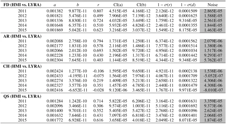
Table 4. Regression statistics applied to the yearly LYRA time series. Statistical parameters are the same as in Table2.
FD (HMI vs. LYRA) a b r CI(a) CI(b) 1 − σ(r) 1 − σ(d) Noise
2011 0.001382 9.877E-11 0.807 4.515E-05 4.168E-12 2.126E-12 0.0001509 2.865E-05
2012 0.001821 5.476E-11 0.499 7.906E-05 7.139E-12 3.640E-12 0.0001625 1.588E-05
2013 0.001336 8.830E-11 0.724 4.032E-05 3.449E-12 1.759E-12 9.316E-05 2.561E-05
2014 0.001648 6.357E-11 0.510 5.932E-05 4.826E-12 2.461E-12 0.0001355 1.844E-05
2015 0.001869 5.042E-11 0.623 3.216E-05 3.037E-12 1.549E-12 8.175E-05 1.463E-05
AR (HMI vs. LYRA)
2011 0.002088 2.758E-10 0.794 1.731E-05 1.250E-11 6.374E-12 0.0001562 2.079E-06
2012 0.002177 1.831E-10 0.578 2.116E-05 1.486E-11 7.577E-12 0.0001514 1.380E-06
2013 0.002066 2.012E-10 0.693 1.502E-05 9.720E-12 4.956E-12 0.0001034 1.517E-06
2014 0.002228 1.233E-10 0.430 2.196E-05 1.317E-11 6.714E-12 0.0001442 9.293E-07
2015 0.002304 7.645E-11 0.403 1.144E-05 8.519E-12 4.344E-12 9.348E-05 5.762E-07
CH (HMI vs. LYRA)
2011 0.002424 1.277E-10 -0.106 1.595E-05 9.650E-11 4.921E-11 0.0002138 1.538E-06
2012 0.002433 -4.195E-11 -0.075 1.564E-05 7.976E-11 4.067E-11 0.0001709 -5.052E-07
2013 0.002274 3.576E-10 0.219 1.409E-05 5.213E-11 2.658E-11 0.0001322 4.306E-06
2014 0.002327 3.577E-10 0.351 1.457E-05 4.785E-11 2.440E-11 0.0001479 4.308E-06
2015 0.002416 -6.652E-11 -0.028 9.120E-06 3.465E-11 1.767E-11 9.971E-05 -8.010E-07
QS (HMI vs. LYRA)
2011 0.001284 1.242E-10 0.714 5.822E-05 6.206E-12 3.164E-12 0.0001631 3.359E-05
2012 0.002096 3.466E-11 0.306 9.574E-05 1.003E-11 5.116E-12 0.0001692 9.373E-06
2013 0.001400 9.701E-11 0.552 5.405E-05 5.427E-12 2.768E-12 0.0001096 2.624E-05
2014 0.001632 7.646E-11 0.431 7.097E-05 6.818E-12 3.476E-12 0.0001401 2.068E-05
2015 0.001772 6.928E-11 0.616 3.658E-05 4.018E-12 2.049E-12 8.071E-05 1.874E-05
The correlation analysis between LYRA and the full-disk magnetic flux density does not show a strong correlation. When executing the analysis for yearly periods, a high correlation is found for 2011 (r = 0.80) and for 2013 (r = 0.72), which indi-cates that the variation in the disk-integrated magnetic field mod-ulates the variations of the spectral irradiance as observed with
the LYRA aluminium channel. Further investigations with alter-native instrumentation is needed to achieve a conclusive result.
In this work we discussed in detail the feasibility and us-age of EUV observations to measure irradiance fluctuations. The observations from AIA allow us to segment the images into different coronal features and to compare the corresponding
0 1×10⁶ 2×10⁶ 3×10⁶ 4×10⁶
Magnetic Flux Density 0 1×10⁸ 2×10⁸ 3×10⁸ 4×10⁸ 5×10⁸ DN/s R=0.93
HMI eAR vs AIA AR, Integrated Intensity
0 2×10⁵ 4×10⁵ 6×10⁵ 8×10⁵
Magnetic Flux Density 0 1×10⁸ 2×10⁸ 3×10⁸ 4×10⁸ DN/s R=0.89
HMI CH vs AIA CH, Integrated Intensity
6.0×10⁶ 8.0×10⁶ 1.0×10⁷ 1.2×10⁷ 1.4×10⁷
Magnetic Flux Density 8.0×10⁸ 1.0×10⁹ 1.2×10⁹ 1.4×10⁹ 1.6×10⁹ DN/s R=0.52
HMI QS vs AIA QS, Integrated Intensity
8.0×10⁶ 1.0×10⁷ 1.2×10⁷ 1.4×10⁷ 1.6×10⁷
Magnetic Flux Density 1.4×10⁹ 1.6×10⁹ 1.8×10⁹ 2.0×10⁹ 2.2×10⁹ 2.4×10⁹ 2.6×10⁹ DN/s R=0.63
HMI DISK vs AIA Disk, Integrated Intensity
8.0×10⁶ 1.0×10⁷ 1.2×10⁷ 1.4×10⁷ 1.6×10⁷
Magnetic Flux Density 0.0020 0.0025 0.0030 0.0035 0.0040 W/m^2 R=0.57
HMI DISK vs LYRA Ch3
8.0×10⁶ 1.0×10⁷ 1.2×10⁷ 1.4×10⁷ 1.6×10⁷ DN/s 0 50 100 150 200 250 #sunspots R=0.52
AIA DISK vs Sunspot Number
Fig. 8.Scatter plots of integrated intensities over the AIA coronal features against the respective HMI magnetic flux density, as in Fig.7.
photospheric LOS magnetic field derived from HMI magne-tograms. This study also shows that the automated identifica-tion and segmentaidentifica-tion of the solar images and magnetograms are very useful in reconstructing the SSI variations.
Acknowledgements. The authors would like to thank the PROBA2 science
cen-tre, located at the Royal Observatory of Belgium (ROB) in Brussels for providing LYRA and SWAP data taken from January 2011 to January 2016. The sunspot numbers were downloaded from SIDC-SILSO, Royal Observatory of Belgium, Brussels. We also thank Solar Dynamic Observatory (SDO) of National Aero-nautics and Space Administration (NASA) for providing AIA and HMI data taken from January 2011 to January 2016. A part of this research work was done at the Indian Institute of Astrophysics when R. Kariyappa (RK) was in regular service. J.J.Z. and R.K. would like to express their sincere thanks to Dr. B.G. Vijayasimha Reddy and Dr. T. Yella Reddy for their encouragement and support on this research. Finally, the authors would like to thank the Faculty of ESA’s Science Support Office for the financial support provided. The authors like to thank the reviewer for the constructive comments and suggestions that improved the manuscript.
References
Babcock, H. W., & Babcock, H. D. 1955,ApJ, 121, 349
Ball, W. T., Unruh, Y. C., Krivova, N. A., Solanki, S., & Harder, J. W. 2011,
A&A, 530, A71
Barra, V., Delouille, V., & Hochedez, J.-F. 2008,Adv. Space Res., 42, 917
Barra, V., Delouille, V., Kretzschmar, M., & Hochedez, J.-F. 2009,A&A, 505,
361
BenMoussa, A., Gissot, S., Schühle, U., et al. 2013,Sol. Phys., 288, 389
Berghmans, D., Hochedez, J. F., Defise, J. M., et al. 2006,Adv. Space Res., 38,
1807
Bertello, L., Pevtsov, A., Tlatov, A., & Singh, J. 2016,Sol. Phys., 291, 2967
Boerner, P., Edwards, C., Lemen, J., et al. 2012,Sol. Phys., 275, 41
Couvidat, S., Schou, J., Hoeksema, J. T., et al. 2016,Sol. Phys., 291, 1887
Dominique, M., Hochedez, J.-F., Schmutz, W., et al. 2013,Sol. Phys., 286, 21
Ermolli, I., Solanki, S. K., Tlatov, A. G., et al. 2009,ApJ, 698, 1000
Ermolli, I., Shibasaki, K., Tlatov, A., & van Driel-Gesztelyi, L. 2014,
Space Sci. Rev., 186, 105
Fontenla, J. M., Curdt, W., Haberreiter, M., Harder, J., & Tian, H. 2009,ApJ,
707, 482
Fontenla, J. M., Codrescu, M., Fedrizzi, M., et al. 2017,ApJ, 834, 54
Foukal, P., & Lean, J. 1988,ApJ, 328, 347
Fröhlich, C., Romero, J., Roth, H., et al. 1995,Sol. Phys., 162, 101
Haberreiter, M. 2011,Sol. Phys., 274, 473
Haberreiter, M., Delouille, V., Mampaey, B., et al. 2014,J. Space Weather Space
Clim., 4, A30
Harvey, K. L., & White, O. R. 1999,J. Geophys. Res., 104, 19759
Hochedez, J.-F., Schmutz, W., Stockman, Y., et al. 2006,Adv. Space Res., 37,
303
Hoeksema, J. T., Liu, Y., Hayashi, K., et al. 2014,Sol. Phys., 289, 3483
Howard, R. 1959,ApJ, 130, 193
Jaeggli, S. A., & Norton, A. A. 2016,ApJ, 820, L11
Kariyappa, R. 2000,JA&A, 21, 293
Kariyappa, R. 2008,JA&A, 29, 159
Kariyappa, R., & Pap, J. M. 1996,Sol. Phys., 167, 115
Kopp, G., & Lean, J. L. 2011,Geophys. Res. Lett., 38, L01706
Kumara, S. T., Kariyappa, R., Dominique, M., et al. 2012,Adv. Astron., 2012, 5
Kumara, S. T., Kariyappa, R., Zender, J. J., et al. 2014,A&A, 561, A9
Lean, J. 1987,J. Geophys. Res., 92, 839
Leighton, R. B. 1959,ApJ, 130, 366
Livingston, W., Wallace, L., White, O. R., & Giampapa, M. S. 2007,ApJ, 657,
1137
Ortiz, A., & Rast, M. 2005,Mem. Soc. Astron. Ital., 76, 1018
Pesnell, W. D., Thompson, B. J., & Chamberlin, P. C. 2012,Sol. Phys., 275, 3
Pevtsov, A. A., Fisher, G. H., Acton, L. W., et al. 2003,ApJ, 598, 1387
Preminger, D., Nandy, D., Chapman, G., & Martens, P. C. H. 2010,Sol. Phys.,
264, 13
Prša, A., Harmanec, P., Torres, G., et al. 2016,AJ, 152, 41
Raftery, C. L., Bloomfield, D. S., Gallagher, P. T., et al. 2013,Sol. Phys., 286,
111
Rottman, G. J., Woods, T. N., & McClintock, W. 2006,Adv. Space Res., 37,
201
Schmutz, W., Fehlmann, A., Finsterle, W., Kopp, G., & Thuillier, G. 2013,AIP
Conf. Ser., 1531, 624
Schrijver, C. J. 1983,A&A, 127, 289
Schrijver, C. J., & Harvey, K. L. 1989,ApJ, 343, 481
Seaton, D. B., Berghmans, D., Nicula, B., et al. 2013,Sol. Phys., 286, 43
Skumanich, A., Smythe, C., & Frazier, E. N. 1975,ApJ, 200, 747
Solanki, S. K. 2003,A&ARv, 11, 153
Stepanov, V. E., & Petrova, N. N. 1959,Izv. Krymsk. Astrofiz. Observ., 21,
352
Tamhane, A., & Dunlop, D. 2000, Statistics and Data Analysis: From Elementary to Intermediate (Pearson)
Verbeeck, C., Delouille, V., Mampaey, B., & De Visscher, R. 2014,A&A, 561,
A29
Veselovsky, I. S., Zhukov, A. N., Dmitriev, A. V., et al. 2001,Sol. Phys., 201, 27
Wenzler, T., Solanki, S. K., Krivova, N. A., & Fröhlich, C. 2006,A&A, 460,
583
Worden, J. R., White, O. R., & Woods, T. N. 1998,ApJ, 496, 998
Yalim, M. S., & Poedts, S. 2014,Adv.n Astron., 2014, 957461
Yeo, K. L., Krivova, N. A., & Solanki, S. K. 2014a,Space Sci. Rev., 186, 137
Yeo, K. L., Krivova, N. A., Solanki, S. K., & Glassmeier, K. H. 2014b,A&A,