HAL Id: hal-02324427
https://hal.archives-ouvertes.fr/hal-02324427
Submitted on 26 Jun 2020
HAL is a multi-disciplinary open access
archive for the deposit and dissemination of
sci-entific research documents, whether they are
pub-lished or not. The documents may come from
teaching and research institutions in France or
abroad, or from public or private research centers.
L’archive ouverte pluridisciplinaire HAL, est
destinée au dépôt et à la diffusion de documents
scientifiques de niveau recherche, publiés ou non,
émanant des établissements d’enseignement et de
recherche français ou étrangers, des laboratoires
publics ou privés.
Mark Wieczorek, Mikael Beuthe, Attilio Rivoldini, Tim van Hoolst
To cite this version:
Mark Wieczorek, Mikael Beuthe, Attilio Rivoldini, Tim van Hoolst. Hydrostatic Interfaces in Bodies
With Nonhydrostatic Lithospheres. Journal of Geophysical Research. Planets, Wiley-Blackwell, 2019,
124 (5), pp.1410-1432. �10.1029/2018JE005909�. �hal-02324427�
Mark A. Wieczorek1 , Mikael Beuthe2 , Attilio Rivoldini2 , and Tim Van Hoolst2
1Université Côte d'Azur, Observatoire de la Côte d'Azur, CNRS, Laboratoire Lagrange, Nice, France,2Royal Observatory
of Belgium, Brussels, Belgium
Abstract
Below the lithospheres of the terrestrial planets, dwarf planets, and moons, density interfaces adjust over geologic time to align with surfaces of constant gravitational potential. It is well known that the shape of such hydrostatic surfaces is controlled by the pseudo-rotational potential, tidal potential, and the induced potential of nonspherical density interfaces in the body. When a lithosphere is present, however, additional gravitational terms must be considered that arise from, for example, surface relief and crustal thickness variations. A first-order formalism is presented for calculating the shape of hydrostatic density interfaces beneath the lithosphere when the gravity field and surface shape of the body are known. Using an arbitrary discretized density profile, the shapes are obtained by solving a simple matrix equation. As examples, lithospheric gravity anomalies account for about 10% of the relief along hydrostatic interfaces in Mars, whereas for the Moon, the lithospheric gravity is the dominant contributor to the core shape. Spherical harmonic degree-1 mass anomalies in the lithosphere generate degree-1 relief along the core-mantle boundary, and for Mars and the Moon, the core is offset from the center of mass of the body by about 90 m. The moments of inertia of the core of these bodies are also misaligned with respect to the principal moments of the entire body. An improved crustal thickness map of Mars is constructed that accounts for gravity anomalies beneath the lithosphere, and the consequences of core relief on the Martian free core nutation are quantified.Plain Language Summary
The shapes of the solid planets and moons are largely hydrostatic and are determined by their rotation rate. If the body has gravity anomalies that arise from within a rigid lithosphere, these will act to perturb the shape of hydrostatic density interfaces beneath the lithosphere, such as the core-mantle boundary. We present a method to compute the shape of density interfaces beneath the lithosphere when the gravity field of the body is known. As examples of our technique, we compute the shape of the core-mantle boundary for Mars and the Moon, both of which are shown to have important contributions that arise from the lithosphere. We also generate a new crustal thickness map that accounts for gravity anomalies generated beneath the lithosphere.1. Introduction
The problem of calculating the shape and gravity field of a rotating hydrostatic body subject to tides is a classic one that goes back to the work of Clairaut (1743). Though the problem involves only a simple force balance, in practice, the general solution for a rapidly rotating body with nonnegligible flattening is a diffi-cult one. A first-order treatment is often sufficient for many problems in planetary science, but higher-order methods can become necessary when treating fast-rotating objects such as Jupiter. Several methods based on different approaches have been developed to solve for the shape of density interfaces within a fluid object that take into account nonlinear effects to both second and higher order, with notable examples including the work of Kopal (1960), Lanzano (1982), Zharkov and Trubitsyn (1978), Chandrasekhar (1969), and Hubbard (2013). Applications of these techniques are common in planetary science (e.g., Chambat et al., 2010; Ermakov et al., 2017; Nakiboglu, 1982; Rambaux et al., 2015; Wisdom & Hubbard, 2016).
It is quite natural to invoke the hypothesis of hydrostatic equilibrium for objects that have no surface strength, such as the Sun and the giant planets of our solar system. When viewed from afar, even solid bodies appear to be approximately in hydrostatic equilibrium, with the flattening depending directly on the rota-tion rate and interior density profile (e.g., Iess et al., 2010; Park et al., 2016; Schubert et al., 2004; Smith et al., 1999). Nevertheless, as one approaches the terrestrial planets, geologic processes lead to the development of
Key Points:
• The terrestrial planets and moons are not in hydrostatic equilibrium and contain mass anomalies in their lithospheres
• The lithosphere generates a gravitational potential that affects the shape of deep interfaces that are hydrostatic
• Hydrostatic interfaces deviate by about 10% for Mars with respect to those for an entirely fluid planet and even more for the Moon
Correspondence to: M. A. Wieczorek, [email protected]
Citation:
Wieczorek, M. A., Beuthe, M., Rivoldini, A., & Van Hoolst, T. (2019). Hydrostatic interfaces in bodies with nonhydrostatic lithospheres. Journal
of Geophysical Research: Planets, 124. https://doi.org/10.1029/2018JE005909
Received 23 DEC 2018 Accepted 21 MAR 2019
Accepted article online 1 APR 2019 Author Contributions
Conceptualization: Mark A. Wiec-zorek
Data curation: Mark A. Wieczorek Methodology: Mark A. Wieczorek, Mikael Beuthe, Attilio Rivoldini Software: Mark A. Wieczorek Validation: Mark A. Wieczorek, Mikael Beuthe, Attilio Rivoldini Writing - Original Draft: Mark A. Wieczorek, Mikael Beuthe, Attilio Rivoldini
Formal Analysis: Mark A. Wieczorek Investigation: Mark A. Wieczorek Resources: Mark A. Wieczorek Visualization: Mark A. Wieczorek Writing - review & editing: Mark A. Wieczorek, Mikael Beuthe, Attilio Rivoldini
©2019. American Geophysical Union. All Rights Reserved.
mass anomalies in the strong outer portion of the body, and these mass anomalies create large gravitational anomalies (for a review, see Wieczorek, 2015). This strong outer portion of the planet, referred to as the lithosphere, can support deviatoric stresses over geologic time, and thus, these mass anomalies will not be in hydrostatic equilibrium. In contrast, the deep interiors of the terrestrial planets, where the temperatures are elevated and rocks deform by creeping viscous flow, are expected to be in hydrostatic equilibrium. As is the case with rotational and tidal potentials, the gravitational potential of mass anomalies in the lithosphere should play a role in determining the shapes of hydrostatic surfaces at depth.
A few studies have recognized the importance of accounting for lithospheric gravitational anomalies when calculating the hydrostatic shape of the core of a planet. In a study by Meyer and Wisdom (2011), long-wavelength lithospheric gravitational anomalies of spherical harmonic degree 2 and order 0 were included when calculating the hydrostatic shape of the core of the Moon. It was found that the core flatten-ing should be about 10 times larger than that predicted for an entirely fluid planet. This excess flattenflatten-ing is consistent with analyses of lunar laser ranging (LLR) data, and Dumberry and Wieczorek (2016) showed that this could have an important influence on the rotational state of a putative solid inner core. In a study by Le Bars et al. (2011), the lithospheric degree 2 and order 2 gravity field was used to determine the equato-rial ellipticity of the lunar core, and this was found to be about 5 times larger than that for an entirely fluid planet. With the computed ellipticity, short-lived episodes of nonsynchronous rotation and/or librations of the mantle (generated by impacts) were shown to be sufficient to excite inertial instabilities in the fluid core, potentially powering a short-lived dynamo. Dumberry et al. (2013) computed the hydrostatic ellipticity of the core of Mercury and showed that this affected the librational signature of the planet. A few studies have considered the shapes of deep hydrostatic interfaces in Titan, Enceladus, and Dione when inverting the observed gravity field and librations for ice shell thickness (Baland et al., 2014; Beuthe et al., 2016; Hoolst et al., 2016; Lefevre et al., 2014). Finally, we note that Zharkov et al. (2009) considered the effects of litho-spheric mass anomalies on the degree-2 shape of the Martian core but by using an approach that considered elastic deformations.
In this study we develop a first-order technique for computing the shape of density interfaces beneath the lithosphere of a planet when the gravity field of the body is known. The approach is to calculate the potential on discrete hydrostatic density interfaces in the object, accounting explicitly for the gravitational potential that results from rotation, tides, and mass anomalies in the lithosphere. The lithospheric anomalies are modeled as being nonhydrostatic and as arising from two sources: one that is a result of relief at the surface and another that results from mass anomalies at a specified depth within the lithosphere (typically, the base of the crust). The relief along all interfaces is solved simultaneously by requiring the potential to be constant along hydrostatic interfaces and by requiring the sum of the gravitational attraction of all interfaces to be equal to the observed value. The problem can be expressed as a set of linear equations, and the solution is determined by solving a simple matrix equation, in contrast to Clairaut's second-order differential equation. Our approach is shown to be more accurate than approaches that are first order in the ratio of centrifugal to gravitational forces due to the inclusion of an extra term in the rotational potential. Finally, at least for the case of Mars and the Moon, we demonstrate that the magnitude of higher-order terms is negligible in comparison to nonhydrostatic lithospheric effects.
In this paper, we first describe the methodology for computing the relief of hydrostatic interfaces beneath the lithosphere. This includes calculating the gravitational potential along an interface, requiring the potential to be constant along hydrostatic interfaces, and also requiring that the predicted gravity matches the obser-vations. Following this, we validate our technique by comparing our results for an entirely fluid body with those obtained from a second- and third-order theory of figures for Mars and Ceres. Next, we demonstrate the utility of our approach for several problems related to Mars and the Moon. For Mars, we first compute the relief along hydrostatic density interfaces in both the core and mantle. Then using these results, we compute a new global crustal thickness map of the planet that accounts for the gravitational attraction of hydrostatic interfaces beneath the lithosphere. These global crustal thickness models will benefit from data that are being collected by the InSight seismometer (Lognonné et al., 2019; Smrekar et al., 2019). Following this, we then quantify how the lithospheric mass anomalies affect the free core nutation period of Mars that will be measured by the InSight spacecraft (Folkner et al., 2018). For the Moon, we compute the shape of the core-mantle interface, showing that the core is not aligned with the principal axes of the Moon and that the core is slightly offset from its center of mass. These results have implications for the interpretation of lunar
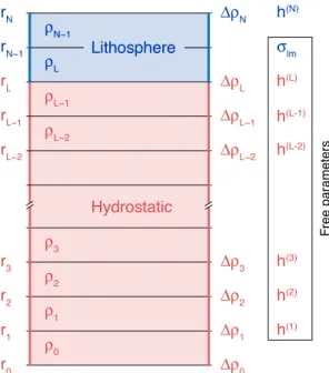
Figure 1. Schematic illustration of the interior structure of the body. ri
denotes the interfaces of constant density layers,𝜌iis the density between two interfaces,𝛥𝜌iis the density contrast at interface i, and h(i)is the relief of interface i. r0corresponds to the center of the planet, rLcorresponds to the shallowest interface that is entirely hydrostatic, rNis the radius of the surface, and the index L corresponds to N−2. In practice, rLcorresponds to rN−T, where T is the maximum thickness of the lithosphere. A nonhydrostatic mass sheet𝜎lmis placed at rN −1within the lithosphere. The radii ri, densities𝜌i, density contrasts𝛥𝜌i, and surface relief h(N)are all
treated as known quantities, whereas h(1)to h(L)and𝜎lmare to be
determined.
laser ranging data, as well as the generation of a dynamo in its past. Finally, we conclude by summarizing the main results of the paper.
2. Hydrostatic Relief With a Lithosphere
In this section, the relief along hydrostatic interfaces within a body is computed when the object contains a nonhydrostatic lithosphere. In the first subsection, expressions are given for the gravitational potential along arbitrary density interfaces in the body. In the second subsection, the assumption of hydrostatic equilibrium is invoked, which requires that the gravitational potential be constant along each hydrostatic interface. This allows to write the coupled equations in matrix form, allowing for a simple resolution of the problem. In the third section, we introduce a cor-rection for the degree-4 terms that are a result of the large amplitudes of the degree-2 shape of the planet. Finally, we describe how this approach can be modified when tidal potentials for a synchronously locked satel-lite are considered. Our methodology treats perturbations in relief with respect to a reference sphere to first order and retains all terms that are linear in the spherical harmonic coefficients of the relief. The main results of this section are given by equations (31)–(34).
2.1. Gravitational Potential Along an Interface
In a reference frame that is fixed to a rotating body, the potential along an interface r(𝜃, 𝜙) can be decomposed into several components:
U = U+ 0 +U − 0 +U ++U−+U rot+Ulith. (1) The first two terms correspond to the gravitational potential of the unper-turbed spherical symmetric reference state from mass below, U+
0, and above, U−
0, an arbitrary observation point. The next two terms correspond to the contribution from relief along each density interface below, U+, and above, U−, the observation point. U
rotcorresponds to the contribution from the rotational potential, and Ulithis the potential derived from the nonhydrostatic lithosphere.
To facilitate the derivations of the above terms, the planet will be described by a spherically symmetric reference 1-dimensional density profile that is composed of N constant density layers𝜌ibounded by constant
radii riand ri+ 1(see Figure 1):
𝜌(r) = 𝜌i for ri≤ r < ri+1, (2)
where the center and surface of the body correspond to r0and rN, respectively. Each interface i will be perturbed from this reference state, with its shape given by
r(i)(𝜃, 𝜙) = r i+ ∞ ∑ l=1 l ∑ m=−l h(lmi)Ylm(𝜃, 𝜙), (3)
where Ylmis the real spherical harmonic of degree l and order m, normalized using the geodesy 4𝜋
con-vention (e.g., Wieczorek & Meschede, 2018), and hlmis the associated spherical harmonic coefficient. Each
interface i is also associated with a density contrast
Δ𝜌i=𝜌i−1−𝜌i. (4)
Given that the density of the atmosphere above the surface of a terrestrial body is negligible when compared to rock, we make the approximation that𝜌Nis 0 and set𝛥𝜌N = 𝜌N −1. Furthermore, for the first interface at the center of the planet, we define𝛥𝜌0 = 0. For brevity of notation, the angular dependence of all functions will be dropped when there is no confusion.
The planet will be assumed to be in hydrostatic equilibrium for all interfaces where i ≤ L = N − 2. Above this, there will be three-dimensional variations in density within the lithosphere that result from surface
topography, lateral variations in crustal thickness, and lateral variations in crustal and upper mantle density. The thickness of the lithosphere of a planet is not constant, and in practice, the interface rLwill be defined
as rN − T, where T is the maximum lithospheric thickness. The interface rL could be thought of as the
uppermost interface of the asthenosphere that is entirely hydrostatic. For simplicity, we will sometimes refer to everything above the interface rLas being the “lithosphere,” but we emphasize that some regions above
this interface could in fact be hydrostatic where the real lithospheric thickness is thinner than T.
The lithospheric signal will be treated as being derived from two separate interfaces. The first interface corresponds to the known surface relief at average radius rN, where a constant density contrast of𝛥𝜌N = 𝜌N −1will be assumed. The remainder of the gravity signal will be treated as arising from a single mass sheet at an average radius rN −1that lies between the surface and rLand which encompasses all other unknown
variations in density within the lithosphere. In practice, the average depth of this interface will be chosen to be equal to the average thickness of the crust of the body.
Before continuing, we note that lateral variations in density could in fact exist in the deep mantle and that nonhydrostatic relief could potentially exist at the core-mantle boundary (e.g., McKinnon, 2013; Wu & Wahr, 1997). For example, mantle convection could give rise to three-dimensional lateral variations in mantle temperature and mantle composition (e.g., Romanowicz, 2003), as well as dynamic topography at the core-mantle boundary (e.g., Defraigne et al., 2001). Unfortunately, beyond Earth, we have few (if any) constraints on the three-dimensional interior structure of the other planets and moons. Thus, in the spirit of the first-order analysis that follows and combined with a paucity of constraints on the interior structures of the terrestrial planets and moons, we will simply neglect these effects.
Throughout the following derivations, we will need to describe the gravitational potential associated with relief along a density interface at mean radius ri. For this, we will make use of the equations
U (r) = ⎧ ⎪ ⎪ ⎨ ⎪ ⎪ ⎩ GM r ∞ ∑ l=0 l ∑ m=−l (r i r )l C(lmi)+Ylm(𝜃, 𝜙) for r ≥ ri GM r ∞ ∑ l=0 l ∑ m=−l (r ri )l+1 C(lmi)−Ylm(𝜃, 𝜙) for r < ri, (5)
where C(lmi)represents the spherical harmonic coefficients of the gravitational potential at a reference radius
ri, G is the gravitational constant, and M is the total mass of the body. The superscripts + and −
associ-ated with the potential coefficients are for the cases where the potential is evaluassoci-ated above and below the interface, respectively. To first order in hlm, we have (e.g., Wieczorek, 2015)
C(lmi)= 4𝜋 Δ𝜌ir 2 ih (i) lm M(2l + 1) , (6) with C+ lmand C −
lmbeing equal. Only later when calculating the gravitational attraction of the surface relief
will higher-order terms be considered.
When evaluating the potential along a density interface, it will be necessary to evaluate the radius of the relief of this surface raised to the nth power in terms of spherical harmonics. Starting with equation (3), the first-order Taylor expansion of this quantity with respect to the (small) nonspherical shape is
[ r(i)(𝜃, 𝜙)]n=rn i ( 1 + ∞ ∑ l=1 l ∑ m=−l h(lmi) ri Ylm )n ≃rn i ( 1 + n ∞ ∑ l=1 l ∑ m=−l h(lmi) ri Ylm ) . (7)
In the subsequent derivations, all terms involving products of hlmhl′m′will be neglected, given their small
magnitudes. As a result of this, there will be no coupling between terms involving two different spherical harmonic degrees or two different angular orders, and it will be possible to resolve the system of linear equations separately for each degree and order. Thus, when analyzing a single degree l and order m, the above equation can be reduced to
[ r(i)(𝜃, 𝜙)]n≃rni ( 1 + nh (i) lm ri Ylm ) . (8)
Though this study uses a first-order approach when calculating the relief along hydrostatic interfaces, it will be shown later that the influence of the nonhydrostatic component of the gravity field is considerably larger than the differences between first-order and higher-order formulations.
In the following subsections, we derive expressions for each of the terms in equation (1) along the interfaces that are assumed to be in hydrostatic equilibrium. Then we impose the condition of hydrostatic equilibrium by requiring the potential along each of these interfaces to be constant.
2.1.1. U0+and U0−
We start by considering an unperturbed reference state that corresponds to a spherically symmetric mass distribution. The potential will be computed on an arbitrary nonspherical surface i, considering the grav-itational potential that arises from mass both above, U0(i)−, and below the surface, U0(i)+. The gravitational potential at radius r resulting from the mass beneath the observation point is simply
U+ 0(r) =
G M(r)
r , (9)
where M(r) is the total mass beneath radius r. The total mass beneath radius r, where r is closest to and larger than ri, is M(r) = i ∑ 𝑗=1 4𝜋 𝜌𝑗−1 3 ( r3 𝑗−r3𝑗−1 ) +4𝜋 𝜌i 3 ( r3−r3 i ) . (10)
Using the first-order approximation of 1∕r and r3from equation (8), the potential on the interface is
U0(i)+= G ri ( 1 −h (i) lm ri Ylm ) [ M(ri) +4𝜋 𝜌i 3 { r3 i ( 1 + 3h (i) lm ri Ylm ) −r3 i }] . (11)
We are interested only in that part of the potential that varies along the interface. Keeping only those terms that depend on Ylmand that are also linear in hlmyields
Ulm,0(i)+ = −GM(ri) h(lmi) r2 i +4𝜋 G𝜌irih (i) lm. (12)
Next consider the gravitational potential from mass above the observation point with respect to the 1-dimensional reference state. The potential of a constant density finite-thickness spherical shell defined by radii r1and r2is shown easily to be (e.g., Blakely, 1995)
U−
0 =2𝜋 G𝜌i(r22−r 2
1), (13)
where𝜌iis the density of the shell. Summing from r to the surface rNgives
U0(i)−= N−1 ∑ 𝑗=i+1 2𝜋 G𝜌𝑗(r2 𝑗+1−r2𝑗) +2𝜋 G𝜌i(r2i+1−r 2). (14)
Using the definition of r for a single harmonic Ylmand retaining only those terms that depend upon this
harmonic yields
Ulm,0(i)− = −4𝜋 G𝜌irih
(i)
lm. (15)
Combining the potential from mass above and below the observation point yields
Ulm,0(i)++Ulm,0(i)− = −GM(ri) h(lmi)
r2
i
2.1.2. U+and U−
Next consider the gravitational potential from the nonspherically symmetric mass distributions related to relief along all hydrostatic interfaces below and including interface i, where i ≤ L. The potential at radius
rfor a single harmonic is given by
U+(r) = i ∑ 𝑗=1 GM r (r 𝑗 r )l4𝜋 Δ𝜌 𝑗r𝑗2h(lm𝑗) M(2l + 1) Ylm, (17)
where r ≥ ri. Since these terms are linear in hlm, when evaluating the potential along interface i, we can
simply make the substitution [ r(i)(𝜃, 𝜙)]l= [ ri+h (i) lmYlm(𝜃, 𝜙) ]l ≃rli, (18) which yields Ulm(i)+= i ∑ 𝑗=1 4𝜋 GΔ𝜌𝑗 (2l + 1) ( rl+𝑗2 rl+1 i ) h(lm𝑗). (19)
Next consider the gravitational potential from relief along all hydrostatic interfaces above i and below L + 1. The potential at radius r for a single harmonic is given by
U−(r) = L ∑ 𝑗=i+1 GM r ( r r𝑗 )l+14𝜋 Δ𝜌 𝑗r𝑗2h(lm𝑗) M(2l + 1) Ylm, (20)
where r < ri. When evaluating the potential along interface i, we make the same substitution as above and
arrive at Ulm(i)−= L ∑ 𝑗=i+1 4𝜋 GΔ𝜌𝑗 (2l + 1) ( rl i rl−1 𝑗 ) h(lm𝑗). (21) 2.1.3. Urot
For a reference frame fixed to a rotating body, the pseudo-rotational potential can be expressed as (e.g., Wieczorek, 2015) Urot= 𝜔 2r2sin2𝜃 2 =𝜔 2r2 ( 1 3Y00− 1 3√5 Y20 ) . (22)
Using the first-order approximation of equation (8) for r along interface i yields
Urot(i) = 𝜔 2r2 i 3 − 𝜔2r2 i 3√5 Y20. (23)
Finally, the component of the rotational potential to spherical harmonic degree l and m is
Ulm,rot(i) = −𝜔 2r2
i
3√5𝛿l2𝛿m0,
(24)
where𝛿 is the Kronecker delta function. In this equation, we have ignored terms that are proportional to
𝜔2r
ih
(i)
lm, which are considerably smaller than those proportional to𝜔
2r2
i. These are typically ignored in
treat-ments of hydrostatic equilibrium that are first order in the expansion parameter q = 𝜔2R∕g, where g is the mean gravitational acceleration at the surface of radius R. Regardless, as will be shown in sections 2.3 and 3, given that the degree-2 terms of the relief hlmare often significantly larger than those of the other degrees,
2.1.4. Ulith
The last contribution to the gravitational potential along a hydrostatic interface comes from mass anomalies in the lithosphere. In practice, the lithosphere of a body encompasses both the crust and uppermost portion of the mantle. The gravitational component from the lithosphere will be considered as arising from two sources: the observed surface relief of the body and a mass sheet at an arbitrary depth, here taken to be the crust-mantle interface. The gravitational attraction associated with the surface relief is by far the largest contributor of the two, and the mass sheet accounts for all remaining unmodeled contributions, such as might be due to lateral variations in crustal thickness, porosity, composition, and temperature. Though the mass sheet term could be modeled explicitly under certain simplifying assumptions (such as using constant density layers and/or elastic flexure), the approach chosen here is to lump all these effects into a single term at a prescribed depth and to interpret the origin of this term afterward. It will be shown later that the depth utilized for this effective source layer has only a modest influence on our results.
Given that the gravitational attraction of the surface relief is large (in part because of the high-density con-trast), we will model this contribution using the higher-order approach of Wieczorek and Phillips (1998). In particular, the spherical harmonic coefficients for use in equation (5) are given by
C(lmN)+=4𝜋 Δ𝜌Nr 3 N M(2l + 1) l+3 ∑ n=1 nh(N) lm rn Nn! n ∏ 𝑗=1 (l +4 −𝑗) (l +3) , (25) C(lmN)−=4𝜋 Δ𝜌Nr 3 N M(2l + 1) ∞ ∑ n=1 nh(N) lm rn Nn! n ∏ 𝑗=1 (l +𝑗 − 3) (l −2) , (26)
where the termnh
lmis defined to be the spherical harmonic coefficients of the function h n
(𝜃, 𝜙). Using the same approximation as in the preceding subsections, the contribution of the surface relief to the potential along hydrostatic interfaces is given by
Ulm,lith(i) =GM ( rl i rl+N1 ) C(lmN)−. (27)
The remainder of the contribution to the lithospheric potential is modeled as arising from a mass sheet at average radius rN −1, which is given by
Ulm,lith(i) = 4𝜋 G (2l + 1) ( rl i rl−1 N−1 ) 𝜎(N−1) lm . (28)
In practice,𝜎lmwill be determined by requiring that the total gravitational potential of the body is equal to
the observed potential.
2.2. Hydrostatic Equilibrium
The condition of hydrostatic equilibrium requires that the gravitational potential be constant along inter-faces of constant density. Thus, after summing all components of the gravitational potential, those compo-nents along a density interface that depend upon degree l and order m must be identically zero. Using the equations from the previous sections for all interfaces i ≤ L, this translates to
0 = −GM(ri)h (i) lm r2 i + i ∑ 𝑗=1 4𝜋 GΔ𝜌𝑗 (2l + 1) ( rl+𝑗2 rl+1 i ) h(lm𝑗)+ L ∑ 𝑗=i+1 4𝜋 GΔ𝜌𝑗 (2l + 1) ( rl i rl−1 𝑗 ) h(lm𝑗) −𝜔 2r2 i 3√5𝛿l2𝛿m0 + 4𝜋 G (2l + 1) ( rl i rl−1 N−1 ) 𝜎(N−1) lm +GM ( rl i rl+N1 ) C(lmN)−. (29)
GM R0 C obs lm = L ∑ 𝑗=1 4𝜋 GΔ𝜌𝑗 (2l + 1) ( rl+2 𝑗 Rl+01 ) h(lm𝑗)+ 4𝜋 G (2l + 1) ( rl+N−21 Rl+01 ) 𝜎(N−1) lm +GM ( rl N Rl+01 ) C(lmN)+, (30)
where the observed coefficients are referenced to the radius R0. Equations (29) and (30) can be written in matrix notation for each spherical harmonic of degree l and order m as
A h = b. (31)
Here h is a vector containing the spherical harmonic coefficients of the lithospheric mass sheet and the relief at each interface i (excluding i = 0)
hi= { h(lmi) for 1≤ i ≤ L 𝜎(N−1) lm for i = N − 1, (32)
and the matrix A depends upon the density profile and location of the density interfaces as given by
Ai𝑗= 4𝜋 GΔ𝜌𝑗 (2l + 1) ( rl+𝑗2 rl+1 i ) for𝑗 < i ≤ L = −GM(ri) r2 i +4𝜋 GΔ𝜌iri (2l + 1) for i =𝑗 ≤ L = 4𝜋 GΔ𝜌𝑗 (2l + 1) ( rl i rl−1 𝑗 ) for i< 𝑗 ≤ L = 4𝜋 G (2l + 1) ( rl i rl−1 N−1 ) for𝑗 = N − 1, i ≤ L = 4𝜋 GΔ𝜌𝑗 (2l + 1) ( rl+2 𝑗 Rl+01 ) for i = N − 1, 𝑗 ≤ L = 4𝜋 G (2l + 1) ( rl+2 N−1 Rl+01 ) for i =𝑗 = N − 1. (33)
The vector b contains that part of the rotational contribution that does not depend upon hlm, as well as the
observed gravitational potential coefficient and gravitational potential of the surface relief:
bi= ⎧ ⎪ ⎨ ⎪ ⎩ 𝜔2r2 i 3√5𝛿l2𝛿m0−GM ( rl i rl+1 N ) C(lmN)− for i≤ L GM R0 Cobs lm −GM ( rl N Rl+1 0 ) Clm(N)+ for i = N − 1. (34)
With A and b computed, equation (31) can be solved individually for each spherical harmonic degree and order.
2.3. Corrections to the Degree-2 and Degree-4 Terms
In the treatment of the hydrostatic equilibrium of a planet, the zonal degree-2 surface relief is usually con-siderably larger than the other degrees and orders. In this section, we will consider an additional small term in the rotational potential of equation (23) that will be shown later to improve the accuracy of both the zonal degree-2 and degree-4 solutions for fluid planets.
When expanding equation (22) using the first-order approximation of equation (8), it can be shown that there are additional small terms to the rotation potential,𝛿U, that were previously ignored in equation (23):
𝛿U(i) rot= 2𝜔2r ih (i) lmYlm 3 − 2𝜔2r ih (i) lm 3√5 YlmY20. (35)
Though this contribution to the rotational potential is smaller than that of equation (23) by a factor propor-tional to h(lmi)∕ri, this could be nonnegligible for planets with many kilometers of rotational flattening. The
last term of the above equation involves the product of two spherical harmonic functions, and this itself can be reexpressed as a weighted sum of spherical harmonic functions up to a maximum degree l + 2. In particular, by defining the function p as the product Y20Ylm, we have
p =(YlmY20 ) = l+2 ∑ l′=0 l′ ∑ m′=−l′ pl′m′(20; lm) Yl′m′, (36)
where the coefficients pl′m′(20; lm)are given by
pl′m′(20; lm) = 1 4𝜋 ∫Ω
(
YlmY20)Yl′m′dΩ. (37)
These coefficients can be calculated easily using numerical spherical harmonic expansion techniques (or alternatively, using Clebsch-Gordan coefficients).
In order to obtain a linear solution that does not involve coupling between different degrees and orders, we retain only that component of p from equation (37) that has the same spherical harmonic degree and order as hlm. Under this assumption, the additional contribution to the rotational potential for spherical harmonic
degree l and order m reduces to
𝛿U(i) lm,rot= 2𝜔2r ih (i) lm 3 ( 1 −plm(20; lm)√ 5 ) . (38)
It is straightforward to show that the inclusion of this term modifies only the diagonal elements of the matrix
Ain section 2.2 by the addition of
𝛿Aii= 2𝜔2r i 3 ( 1 −plm(20; lm)√ 5 ) for i≤ L. (39)
Though this small contribution to the rotational potential could be computed for any degree and order, in practice, we will make use only of the zonal degree-2 correction. This term is not included in treatments of hydrostatic equilibrium that are first order in the expansion parameter q = 𝜔2R∕g, and its utility will be assessed in section 3.
As seen in equations (35)–(37), relief hlmalong an interface will generate a small contribution to the
rota-tional potential at degrees other than just degree l. In general, the h20term of a body will be by far the largest as a result of the rotational flattening, and the additional contributions to the rotational potential will thus be the largest for those components that depend upon h20. We will assume that the degree-2 relief of all interfaces has been determined previously by solving the equations of the preceding section. Then, using these terms, a correction will be computed that is applicable when computing the degree-4 relief.
Using the definition of pl′m′(20; lm)in equation (37), the last term of equation (23) for l = 2 can be expanded
as −2𝜔 2r ih (i) 2m 3√5 Y2mY20= − 2𝜔2r ih (i) 2m 3√5 4 ∑ l′=0 l′ ∑ m′=−l′ pl′m′(20; 2m) Yl′m′. (40)
Using the properties of the Clebsch-Gordan coefficients, it can be shown that pl′m′(20; 2m)is nonzero only
when l′is 0, 2, and 4 and when m′ = m. In the previous derivations of this section, only the l′ = 2term was considered. The degree-4 term of equation (40) could be important given the large amplitude of the h2m relief, and these terms should be included in equation (29) when solving for the degree-4 relief. Given that the components of the above equation do not depend upon h4m, it is straightforward to show that it is only necessary to add the correction
𝛿bi= 2𝜔2r ih (i) 2m 3√5 p4m(20; 2m) for l = 4, |m| ≤ 2, i ≤ L, (41)
to the vector b in equation (34). Though this contribution could be computed for all angular orders of degree 4, in practice, we will make use only of the zonal term, which is proportional to the zonal degree-2 term. 2.4. Tidal Potentials
For a reference frame fixed to a satellite that is in synchronous rotation about a central planet, the static part of the tidal potential can be written as (e.g., Wieczorek, 2015)
Utide≃ G Mpr 2 a3 ( − √ 5 10Y20+ 1 4 √ 12 5Y22 ) , (42)
where Mp is the mass of the planet and a is the semimajor axis of the satellite. Using the first-order
approximation for r2, the potential on each interface i is
Utide(i) = ( G Mpr2 i a3 ) ( − √ 5 10Y20+ 1 4 √ 12 5Y22 ) + ( G Mpr2i a3 ) ( − √ 5 5 h(lmi) ri YlmY20+ 1 2 √ 12 5 h(lmi) ri YlmY22 ) . (43)
Following the same approach as in section 2.3, the products of two spherical harmonics are expanded in spherical harmonics, and only those terms that depend on Ylmare retained. The spherical harmonic
coefficients of the potential along interface i can thus be given by
Ulm,tide(i) = ( G Mpri2 a3 ) ( − √ 5 10𝛿l2𝛿m0+ 1 4 √ 12 5𝛿l2𝛿m2 ) +h(lmi) (G M pri a3 ) ( − √ 5 5 plm(20; lm) + 1 2 √ 12 5 plm(22; lm) ) . (44)
It is trivial to modify the elements of the matrix equation (equation (31)) to account for the tidal potential. For the elements of A in equation (33), it is only necessary to modify the diagonal terms
Aii= − GM(ri) r2 i +4𝜋 GΔ𝜌iri (2l + 1) + 2𝜔2r i 3 ( 1 −plm(20; lm)√ 5 ) + (G M pri a3 ) ( − √ 5 5 plm(20; lm) + 1 2 √ 12 5 plm(22; lm) ) for i≤ L, (45)
and for the vector b, the elements are given by the modification
bi= ⎧ ⎪ ⎨ ⎪ ⎩ 𝜔2r2 i 3√5𝛿l2𝛿m0+ G Mpr2i a3 (√ 5 10𝛿l2𝛿m0− 1 4 √ 12 5𝛿l2𝛿m2 ) −GM ( rl i rl+1 N ) C(lmN)− for i≤ L GM R0C obs lm −GM ( rl N Rl+1 0 ) C(lmN)+ for i = N − 1. (46)
It is noted that the term G Mp∕a3is approximately equal to𝜔2when the mass of the satellite is small in
comparison to that of the planet it orbits.
The largest contributions to the shape of a tidally deformed synchronous satellite are generally the terms h20 and h22. Similar to the discussion in section (2.3), these terms could generate small contributions of spherical harmonic degree-4 to the tidal potential. Accounting for these contributions, however, is somewhat more complicated than for the case of the rotational potential, as several of the spherical harmonic degrees and order become coupled. In particular, when considering the relief h20and h22 terms, additional terms to the potential would be generated that are proportional to h20Y22, h20Y42, h22Y20, h22Y40, and h22Y44. These terms will be ignored in this study as they have a small amplitude. Though they are certainly negligible for Earth's Moon (which will be investigated in section 4.4), they could be of importance for application to other satellites, such as Jupiter's moon Io.
Table 1
Observed h20and h40for the Surface of Mars and Predicted Values Assuming Hydrostatic Equilibrium
h20(m) h40(m) Source
−5,966.2 224.7 Observed (MarsTopo2600, Wieczorek, 2015)
−5030.4 — First order (using code of Chambat et al., 2010)
−5,049.3 10.4 Second order (using code of Chambat et al., 2010)
−5,053.9 8.3 This study
−5,030.0 8.2 This study, ignoring equation (39)
3. Validation
The accuracy of the above formalism will be tested against known entirely fluid solutions for Mars and Ceres. We first compute the relief along all interfaces assuming that the bodies are entirely hydrostatic. Then, we compare these solutions with those obtained using the second-order theory of Chambat et al. (2010), which is itself based on Kopal (1960) and Lanzano (1982). Finally, we demonstrate that the surface of Mars is in fact far from hydrostatic equilibrium.
For our model illustrated in Figure 1, when a body has no lithosphere, the radial index corresponding to the index L is equivalent to the index N of the surface. To obtain a purely hydrostatic solution, it is only necessary to make use of the L × L submatrix of A in equation (31). In particular, the last row and column of A and b, which contain the lithospheric terms and known gravity field, are simply discarded. The resulting equations are equivalent to a first-order discretized version of Clairaut's integral equation (see equation 12, p. 185, Jeffreys, 1970), with the exception of the inclusion of the small term proportional to𝜔2h
lmas described in
section 2.3. The equations in Chambat et al. (2010) contain terms of order h2
lmand require the solution of a
second-order differential equation.
For our first test, we make use of a density profile of Mars that is derived from the Mars bulk-silicate compo-sitional model of Taylor (2013). This model (TAAK, see Table 4) has a core radius of 1,791 km and is taken from the Mars reference models presented in Smrekar et al. (2019). The predicted hydrostatic flattening cor-responds to a difference of 17 km between the poles and equator, and the observed values of h20and h40, our predicted values, and those predicted by the first- and second-order hydrostatic theories from the numerical code of Chambat et al. (2010) are given in Table 1.
Somewhat remarkably, our first-order results and the second-order results using the code of Chambat et al. (2010) for the zonal degree-2 surface shape h20are found to differ by only 0.09%. If we were to have ignored the small term of equation (39), our results would be nearly identical to the first-order value from the same code. Our first-order theory provides a value for the zonal degree-4 shape h40that is comparable to the second-order prediction but differs by 21%.
For Mars, it should be emphasized that the observed shape deviates substantially from the predicted hydro-static values. For the zonal degree-2 term, the difference is about 15%, whereas for the zonal degree-4 term,
Table 2
Observed(a−c)for Ceres and Predicted Values for a Uniform Density Body Assuming Hydrostatic Equilibrium
a −c(km) Source
37.2±0.1 Observed (Park et al., 2016)
37.908 First order (Rambaux et al., 2015)
39.561 Second order (Rambaux et al., 2015)
39.739 Third order (Rambaux et al., 2015)
39.764 Exact Maclaurin ellipsoid (Rambaux et al., 2015)
40.431 This study
41.019 l =2, this study
the two differ by a factor of 21. It is thus clear that the nonhydrostatic contribution to the shape of Mars exceeds greatly the small differences between the first- and second-order theories. It is thus not necessary to apply a higher-order hydrostatic theory to a planet like Mars that is far from hydrostatic equilibrium. For Ceres, we test our approach using the constant density model that was tested in Rambaux et al. (2015). Though more realistic density profiles resulting from internal differentiation were also tested in that study, the homogeneous case was found to give the largest discrepancies between the first- and third-order theories of figures. The constant density model is not meant to provide the best fit to the observations and is used here only as a numerical test. In Table 2, we provide the difference in the equatorial and polar axes, a − c, predicted for hydrostatic equilibrium, as well as the measured value of Park et al. (2016). A difference of 1.86 km was found between the exact solution of a Maclaurin ellipsoid and their first-order solution, which corresponds to a relative error of 4.7%.
Using our approach, we find a difference of only 0.67 km for a − c with that predicted for a Maclaurin ellip-soid, which corresponds to a relative error of 1.7%. The better concordance is a result of us having calculated a degree-4 term and having included the correction of equation (39), both of which are generally neglected in first-order theories. If we were to have neglected the degree-4 term, the difference with respect to the exact solution would have increased to 1.26 km (3.2%). If we were to have also neglected the correction of equation (39), our solution would be nearly identical to the first-order solution of Rambaux et al. (2015). Thus, though a higher-order approach may be necessary to model the hydrostatic shape of Ceres for cer-tain applications, for this particular model, our approach provides a value that is more accurate by almost a factor of three in comparison to previous first-order techniques.
4. Applications
The theory developed in section 2 can be applied to any terrestrial planet, dwarf planet, or differentiated asteroid or moon whose gravity field is known. Here we demonstrate several potential applications to Mars and Earth's Moon. First, we calculate the shape of hydrostatic interfaces in Mars, which are shown to be perturbed by the gravitational potential associated with the Tharsis province. Second, we compute the gravitational potential of these interfaces and invert the remaining lithospheric signal for crustal thickness variations. Third, using our computed shape of the core-mantle boundary, we determine how the litho-spheric gravity affects the free core nutation frequency. Finally, we compute the shape of the core-mantle boundary of the Moon, which is important for interpretations of LLR data.
4.1. Mars: Shape of Hydrostatic Interfaces
In calculating the shape of hydrostatic interfaces in the planet Mars, we will make use of the 120 degree and order gravity field GMM-3 of Genova et al. (2016) and the spherical harmonic shape model of Wieczorek (2015), both truncated at degree 90. For the density profile of the planet, we will make use of the model TAAK from Smrekar et al. (2019) that is based on the bulk-silicate compositional model of Taylor (2013) and which has a core radius of 1,791 km (see also Table 4). Only the density profile of this model beneath the maximum depth of the lithosphere is required for our calculations, given that the gravity contribution of the lithosphere is treated separately (see Figure 1). When calculating the gravitational contribution of the surface topography, a crustal density of 2,900 kg/m3will be assumed. A large part of the remainder of the nonhydrostatic mass anomalies in the lithosphere is likely a result of relief along the crust-mantle interface, so we will assume a depth to this interface of 45 km, which is close to the predicted average thickness of the crust (e.g., Neumann et al., 2004; Wieczorek & Zuber, 2004). Though it is likely that a small portion of the lithospheric signal could come from shallower portions of the crust (such as from magmatic intrusions or lateral variations in crustal composition), it is unlikely that significant density anomalies would be present in the lithospheric mantle beneath the crust.
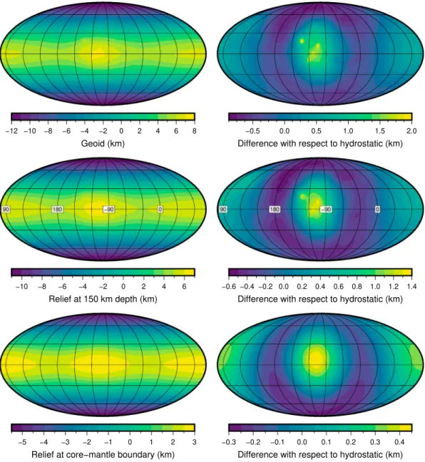
The geoid of Mars (i.e., the shape of an equipotential surface) is plotted in the top row of Figure 2 using the GMM-3 gravity model. In the left column, the heights are referenced to the mean radius of the planet, whereas in the right column, the heights are referenced to the shape predicted if the planet was entirely fluid. In all images, the central meridian is 100◦W, which corresponds to the mean longitude of the Tharsis volcanic province. A difference in elevation of about 17 km is visible from pole to equator, which is primar-ily a result of the rotational flattening of the planet. Nevertheless, as is evident in the right column, there are about 3 km of relief superposed on that predicted for a purely fluid planet. These geoid anomalies are pri-marily a result of the volcanic load of the Tharsis province, several large volcanoes that are superposed on
Figure 2. The geoid of Mars, hydrostatic relief along an interface at 150-km depth, and hydrostatic relief of the
core-mantle boundary. Mass anomalies within the lithosphere were placed at a depth of 45 km, the maximum thickness of the lithosphere was assumed to be 150 km, and the core radius is 1,791 km. The relief is calculated with respect to the mean radius of each interface in the left panel, whereas in the right panel, the relief is calculated with respect to the shape expected for an entirely fluid planet. Images are in a Mollweide projection with a central meridian of 100◦W longitude, which corresponds to the center of the Tharsis province. The color bars for each image are scaled to the minimum and maximum values of the data.
this province (such as Olympus Mons), and the flexural response of the planet to these loads (e.g., Phillips, Zuber, Solomon, et al., 2001). For comparison, the 3 km of geoid relief on Mars is considerably larger than the few hundred meters of relief of Earth's geoid (e.g., Wieczorek, 2015).
The predicted hydrostatic relief at 150-km depth is plotted in the middle row of Figure 2. For this calcula-tion, we assumed a maximum lithospheric thickness of 150 km, which corresponds approximately to the best-fitting elastic thickness of 140 km that was determined beneath the South polar cap using gravity and topography data (Wieczorek, 2008). Nevertheless, we note that this value is shallower than the inferred elas-tic thickness of more than 300 km beneath the North polar cap that is based on radar data (Phillips, Zuber, Smrekar, et al., 2001). The interface at 150-km depth is close to the mass anomalies located at the surface and at 45-km depth, and the computed hydrostatic relief along this interface is found to vary by 2 km (when referenced to that predicted for an entirely fluid planet). This relief is comparable to the 3 km of relief of
Table 3
Low-Degree Spherical Harmonic Coefficients (in Meters) of the Relief Along the Core-Mantle Interface of Mars for Interior Model TAAK
l m hlm hl, − m 0 0 1,791,372.60 1 0 45.53 1 1 3.26 25.58 2 0 −2,361.32 2 1 −2.95 −1.62 2 2 −121.40 68.06 3 0 −10.67 3 1 4.34 20.89 3 2 −10.86 4.43 3 3 24.95 15.13
Note. For an entirely fluid planet, all terms would be zero except h20, which is predicted to be−2,276.36.
the geoid, and the two maps differ only somewhat as a result of the attenuation of the shortest wavelength signals.
The hydrostatic relief at the core-mantle boundary is shown in the bottom row of Figure 2, and the spherical-harmonic coefficients of the core shape are given in Table 3. The largest signal is a zonal com-ponent that has a difference in radius between the poles and equator of about 8 km. At this depth, the gravitational potential from the lithosphere is highly attenuated, and the high-frequency structure associ-ated with the interior of the Tharsis province in the previous images is largely absent. Regardless, as is shown in the right column, even at these depths, there is still about 710 m of relief along the core-mantle bound-ary with respect to that associated for an entirely fluid planet. This relief is almost entirely the result of the degree-2 terms of the lithospheric gravity field. The amplitude of individual degree-4 terms is less than 5 m. We note that the shape of the core of Mars is predicted to have a small degree-1 component. In the above model, this corresponds to an amplitude of 87 m and implies that the core is offset from the center-of-mass of the planet by the same amount. This may at first seem counterintuitive but is easy to explain by use of a simple model. Consider a planet that contains two separate degree-1 mass anomalies at radii r1and r2with respective spherical-harmonic coefficients C1m(1)and C(2)1m. To be in center-of-mass coordinates, the combined gravitational contribution of the two is required to be exactly zero exterior to the planet, and this implies that
C(1)1m= −C(2)1m(r2∕r1). However, if one were to calculate the gravitational potential below these two interfaces, one would find that the degree-1 potential would be nonzero. In fact, the degree-1 potential would be zero everywhere only if the radii of the two interfaces coincided. Using a similar argument, it is easy to show that the principal moments of inertia of the core are not required to be aligned with those of the entire body. In fact, for the TAAK model, we find that the maximum principal moment of the core is inclined by 0.05◦with respect to the mean rotation axis of the planet.
Lastly, we quantify how our results depend upon the assumed crustal density and depth of the lithospheric mass anomalies. Varying the density of the crust from 2,500 to 3,300 kg/m3is found to have only a small effect, with the relief at 150-km depth and the core-mantle interface changing by no more than about 78 m. Modifying the depth of the mass anomalies in the lithosphere, however, has a slightly more important effect. Our nominal case employed a depth of 45 km, which corresponds approximately to the base of the crust, and as extreme end-members, we varied this depth from the surface to 100 km. For the hydrostatic relief at 150-km depth, this caused variations up to 310 m, which corresponds to about 10% of the maximum relief along this interface when referenced to the entirely fluid solution. For the core-mantle boundary, the maximum difference was found to be 143 m, which is about 32% of the maximum relief along this interface when referenced to the entirely fluid solution.
4.2. Mars: Global Crustal Thickness
The main contributions to the observed gravity field of Mars come from the shape of the surface, variations in thickness of the crust, and the hydrostatic flattening of density interfaces in the mantle and core. By
Table 4
Percentage of the Observed C20Potential Coefficient That Is Derived From Hydrostatic Interfaces Beneath the Lithosphere at 150-km Depth
Model name Compositional model Core radius (km) %C20
DWTH Wänke and Dreibus (1988) 1,755 4.3
DWTHC1 Wänke and Dreibus (1988) 1,805 4.5
EH45TC Sanloup et al. (1999) 1,850 5.2
EH45TCC1 Sanloup et al. (1999) 1,718 4.9
EH45THC2 Sanloup et al. (1999) 1,795 4.6
ZGDW Zharkov and Gudkova (2005) 1,798 5.7
DWAK Wänke and Dreibus (1988) 1,781 6.2
LFAK Lodders and Fegley (1997) 1,745 5.6
SAAK Sanloup et al. (1999) 1,762 5.0
TAAK Taylor (2013) 1,791 6.3
Note. Interior reference models are from Smrekar et al. (2019).
making assumptions about the crustal density, average thickness of the crust, and the density profile of the mantle and core, it becomes possible to invert for the relief along the crust-mantle interface and to create a map of how crustal thickness varies laterally. Crustal thickness modeling of this type has been applied to all of the terrestrial planets, the Moon, and some differentiated asteroids (see, e.g., Wieczorek, 2015). The most notable example for Mars is the work of Neumann et al. (2004), with later work by Baratoux et al. (2014) highlighting how uncertainties in the assumed crustal density affect these models.
In this section, we construct a new global crustal thickness model for Mars that takes into account explicitly the gravitational attraction of hydrostatic density interfaces beneath the lithosphere. Previously, Neumann et al. (2004) considered the gravitational contribution of the rotationally flattened core-mantle boundary. This was found to contribute 2% to the observed C20potential coefficient of Mars. Later, Cheung and King (2014) improved upon this by computing the gravitational contribution of all flattened interfaces for a per-fectly fluid planet before inverting for crustal thickness variations. The second-order approach of Chambat et al. (2010) was used to compute the hydrostatic gravity field in their study, but an analysis of their code shows that the contribution from the core-mantle interface was mistakenly counted twice.
In our approach, we compute the gravitational contribution resulting from all hydrostatic interfaces beneath the lithosphere. Though all harmonic degrees and orders will be considered, the largest contributor is for the
C20term. The predicted contribution to the observed value for this harmonic is provided in Table 4 for several density profiles that were employed in Smrekar et al. (2019). As is seen, depending on the assumed density profile, between 4.4% and 6.4% of the observed C20gravity coefficient is a result of hydrostatic interfaces beneath the lithosphere. Only about 2% of the observed value is a result of the core, similar to Neumann et al. (2004), with the remainder being a result of the mantle.
We follow an approach similar to Wieczorek and Phillips (1998) for constructing a global crustal thickness model. First, the gravitational attraction of hydrostatic interfaces beneath 150-km depth was computed using the TAAK density profile, and the gravitational attraction of the surface topography was computed using an assumed density of 2,900 kg/m3. Both of these contributions were then removed from the GMM-3 gravity coefficients of Genova et al. (2016). Next, based on the TAAK reference model, a density of 3,376 kg/m3was assigned to the uppermost mantle, and the approach of Wieczorek and Phillips (1998) was used to invert the remaining gravity field for relief along the crust-mantle interface. A downward continuation filter with an amplitude of 0.5 at degree 50 was employed, all calculations were truncated at degree 90, and gravitational finite-amplitude effects were computed to order 7, which is more than sufficient for the purposes of this work. Lacking seismic constraints, the average thickness of the crust was adjusted iteratively in order to obtain a minimum crustal thickness of 1 km, which was always found to occur in the center of the Isidis impact basin. A thicker minimum crustal-thickness constraint could have been employed, and though not considered here, lateral variations in crustal density could also have been accounted for (see Plesa et al., 2016; Smrekar et al., 2019; Wieczorek et al., 2013).
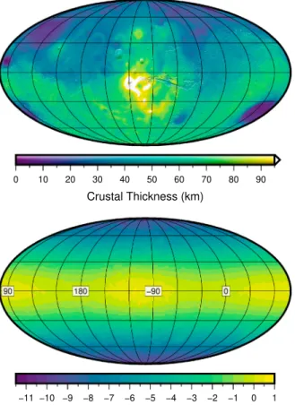
Figure 3. Crustal thickness of Mars. (top) Total crustal thickness, accounting for the gravitational attraction of
hydrostatic interfaces beneath the lithosphere. (middle) Difference in crustal thickness when density interfaces beneath the lithosphere are ignored. (bottom) Difference in crustal thickness when using the hydrostatic shape of density interfaces beneath the lithosphere and the shape of these interfaces predicted for an entirely fluid planet. Images are in a Mollweide projection with a central meridian of 100◦W longitude, which corresponds to the center of the Tharsis province. A shaded relief map of surface topography is overlain on the crustal thickness map in the top image. The color bars for each image are scaled to the minimum and maximum values of the data, with the exception of the top panel where the upper bound is set to 95 km.
Our final crustal thickness model is displayed in the top panel of Figure 3. For this model, the average crustal thickness is 51 km, the predicted thickness at the InSight landing site is 33 km, and the maximum thickness is 111 km. The model is broadly similar to that of Neumann et al. (2004), but as a result of including all hydrostatic interfaces beneath the lithosphere, it differs somewhat by having a different long-wavelength pole-to-equator behavior that results from a different correction to the C20potential harmonic.
Table 5
Principal Moments of Inertia of the Core of Mars for the TAAK Interior Model
Moment Fluid planet Planet with a lithosphere
Ac 0.0254088 0.0254036
Bc 0.0254088 0.0254113
Cc 0.0255172 0.0255199
Note. The principal moments are normalized by MR2, where M and R and the observed mass and mean planetary radius of the planet.
The difference between our model and one that does not include any gravitational contribution from beneath the lithosphere is shown in the middle panel of this figure. The differences are small near the equator, which is a result of the fact that the minimum crustal thickness constraint occurs in the Isidis impact basin that is near the equator. However, the difference in crustal thickness grows substantially to about 11 km at the poles. In particular, at the north pole, the crustal thickness is predicted to be about 38 km when gravity contributions from beneath the lithosphere are considered and about 48 km when they are neglected. Lastly, in the bottom panel of Figure 3, we plot the difference between our crustal thickness model and one that used hydrostatic interfaces beneath the lithosphere computed for an entirely fluid planet. The differences in this case are small, with variations of only 1 km being associated with the degree-2 terms.
4.3. Mars: Free Core Nutations
The time-dependent tidal forcing exerted on the flattened shape of Mars by the Sun, planets, and Martian moons Phobos and Deimos induces periodic variations in its rotation (Dehant et al., 2000). These nutations are superposed on the much longer precession of the spin axis of the planet about the normal to the orbit plane that has a period of about 171,000 years. Since the core of Mars is at least partially fluid, relative rotational motion between the mantle and core can occur. A rotational normal mode called the free core nutation (e.g., Dehant & Mathews, 2015), describing the rotation of the core around a different spin axis than that of the solid mantle, can resonantly amplify the nutations.
Nutations of Mars will be measured by the Rotation and Interior Structure Experiment (RISE) that is part of the InSight mission (Folkner et al., 2018). The instrument measures the relative velocity between the lander and Earth from Doppler shifts of a tracking signal, and it is expected that RISE will determine the nutation period with an error of about 5 days (Folkner et al., 2018). If the shape of the core was known, the radius of the core could be constrained from the free core nutation period (Folkner et al., 2018). Conversely, if the radius of the core were known, for instance, from tidal measurements (Genova et al., 2016; Konopliv et al., 2006), seismic sounding by InSight (Panning et al., 2016), or nutation amplitude measurements by RISE (Folkner et al., 2018), the flattened shape of the core could be constrained.
Using the same reference interior model as in the previous two sections (TAAK), we have computed the three principal moments of inertia of the core, which depend upon the degree-2 core shape (see Table 5). When the core equatorial ellipticity is small compared to its polar flattening, as is the case for our model that considers gravity anomalies in the lithosphere, the frequency of the free core nutation can be expressed as (Van Hoolst & Dehant, 2002)
𝜎FCN = −𝜔 ( A A − Ac ) (𝛼c− ̃𝛽). (47)
In this equation,𝛼cis the dynamical flattening of the core defined as 𝛼c=
Cc− (Ac+Bc)∕2 (Ac+Bc)∕2
. (48)
Ac, Bc, and Ccare the three principal moments of the core, A is the minimum principal moment of the entire planet, and ̃𝛽 = 0.00032 is a compliance that characterizes the core's capacity to deform due to centrifugal acceleration associated with the core rotating about a different axis than the mantle (e.g., Dehant & Mathews, 2015). We compute the moment A by use of the observed precession rate and gravity model of Konopliv et al. (2016). When normalized by MR2, where M is the mass of Mars and R is the mean planetary radius (3,389.5 km), we obtain A∕(MR2)equal to 0.362976. We note that the first term in parentheses is insensitive
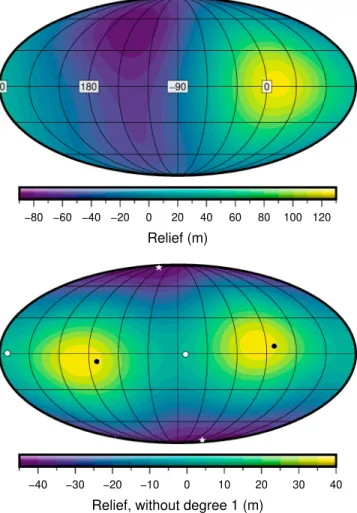
Figure 4. Relief along the core-mantle interface of the Moon with respect to a sphere of radius 330 km. The depth of
the lithospheric mass anomalies was set to 34 km, and the radius of the core was set to 330 km. In the top panel, the total shape of the core is plotted, whereas in the bottom panel, the shape is plotted after removing the degree-1 terms. The axes of the A, B, and C principal moments are plotted using black circles, white circles, and stars, respectively. Images are in a Mollweide projection with a central meridian of 90◦W longitude, and the color bars for each image are scaled to the minimum and maximum values of the data.
to the core shape and that the free core nutation period is linear in𝛼c. Equation (47) is correct up to first order in polar flattening of the core and the whole planet if the planet is biaxial (Van Hoolst et al., 2000). The free core nutation period implied by the core figure that considers mass anomalies in the lithosphere is −232.4 days, whereas the same model using the figure of the core for a completely fluid planet is about 10 days smaller (−241.8 days). This difference is, in principle, large enough to be detected by RISE. This difference of 10 days is almost an entire consequence of the core dynamical flattening,𝛼c, that differs by about 3.7% between the two models. Further corrections due to triaxial effects are below 1 day (Molodensky et al., 2009; Van Hoolst & Dehant, 2002).
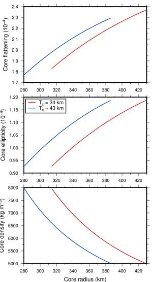
4.4. The Moon: Core Shape
The shape and gravity field of the Moon have long been known to be in a state that is far from hydrostatic equilibrium. Laplace (1799) was the first to note that the observed moments of inertia were inconsistent with being in hydrostatic equilibrium at the current Earth-Moon separation. Sedgwick (1898) and Jeffreys (1915) suggested that the equilibrium shape of the Moon could have been frozen into the lithosphere when the Moon was much closer to Earth in its distant past. Later studies have since attempted to quantify the lunar rotation rate, the Earth-Moon separation, and the time when this “fossil bulge” was acquired (e.g., Garrick-Bethell et al., 2006; Keane & Matsuyama, 2014; Lambeck & Pullan, 1980; Matsuyama, 2013; Qin et al., 2018). Similar to Mars, the nonhydrostatic state of the lithosphere of the Moon will generate a