HAL Id: hal-00878469
https://hal.inria.fr/hal-00878469
Submitted on 30 Oct 2013
HAL is a multi-disciplinary open access
archive for the deposit and dissemination of
sci-entific research documents, whether they are
pub-lished or not. The documents may come from
teaching and research institutions in France or
abroad, or from public or private research centers.
L’archive ouverte pluridisciplinaire HAL, est
destinée au dépôt et à la diffusion de documents
scientifiques de niveau recherche, publiés ou non,
émanant des établissements d’enseignement et de
recherche français ou étrangers, des laboratoires
publics ou privés.
Adjoint-based optimization on a network of discretized
scalar conservation law PDEs with applications to
coordinated ramp metering
Jack Reilly, Walid Krichene, Maria Laura Delle Monache, Samitha
Samaranayake, Paola Goatin, Alexandre Bayen
To cite this version:
Jack Reilly, Walid Krichene, Maria Laura Delle Monache, Samitha Samaranayake, Paola Goatin, et al..
Adjoint-based optimization on a network of discretized scalar conservation law PDEs with applications
to coordinated ramp metering. Journal of Optimization Theory and Applications, Springer Verlag,
2015, 167 (2), pp.733-760. �hal-00878469�
Noname manuscript No. (will be inserted by the editor)
Adjoint-based optimization on a network of discretized scalar
conservation law PDEs with applications to coordinated ramp
metering
Jack Reilly⇤ · Walid Krichene⇤ · Maria Laura Delle
Monache† · Samitha Samaranayake⇤ · Paola Goatin† ·
Alexandre M. Bayen⇤
Submitted: October 23, 2013
Abstract The adjoint method provides a computationally efficient means of calculating the gradient for applications in constrained optimization. In this article, we consider a network of scalar conservation laws with general topology, whose behavior is modified by a set of control parameters in order to minimize a given objective function. After discretizing the corresponding partial differential equation models via the Godunov scheme, we detail the computation of the gradient of the discretized system with respect to the control parameters and show that the complexity of its computation scales linearly with the number of discrete state variables for networks of small vertex degree. The method is applied to solve the problem of coordinated ramp metering on freeway networks. Numerical simulations on the I15 freeway in California demonstrate an improvement in performance and running time compared to existing methods.
Keywords control of discretized PDEs, network of hyperbolic conservation laws, adjoint based
optimization, transportation engineering, ramp metering
1 Introduction
Networks of one-dimensional conservation laws, described by systems of nonlinear first-order hyperbolic partial differential equations (PDEs), are an efficient framework for modeling physical phenomena, such as gas pipeline flow [1], supply chain [2], water channels [3, 4], or freeway traffic evolution [5, 6, 7]. Optimization and control of these networks is an active field of research [8, 9, 10]. More generally, numerous techniques exist for the control of conservation laws, such as, for example, backstepping [11, 12], Lyapunov-based methods [11], and optimal control methods [13, 14, 15].
One such approach, known as the adjoint method, as used in optimal control and estimation of PDE-constrained systems, can be derived in various ways depending on the framework of interest (PDE, dis-cretization of the PDE, or code implementing the disdis-cretization of the PDE). The continuous adjoint method [16, 8, 17, 18] operates directly on the PDE and a so-called adjoint PDE system, which when solved can be used to obtain an explicit expression of the gradient of the underlying optimization problem. Conversely, the discrete adjoint method [19, 8, 10] first discretizes a continuous-time PDE and then requires the solution of a set of linear equations to solve for the gradient. Finally, a third approach exists, which uses automatic differentiation techniques to automatically generate an adjoint solver from the numerical representation of the forward system [20, 21].
While the continuous adjoint formulation results in a compact formulation, better intuition into the system’s sensitivities with respect to the objective, and well-posedness of the control’s solution (when it can be proved), it is often difficult to derive for systems of hyperbolic nonlinear PDEs controlled by boundary conditions, when these boundary conditions have to be written in the weak sense. Additionally, the continuous adjoint must eventually be discretized in order to produce numerical solutions for the optimization problem. Finally, the differentiation of the forward PDE is sometimes problematic due to the lack of regularity of the solution [5, 6] which makes the formal definition of the adjoint problem more difficult. The discrete adjoint approach derives the gradient directly from the discretized system, thus
⇤University of California, Berkeley - California, USA E-mail: jackdreilly@berkeley.edu ·
avoiding working directly with weak boundary conditions in the continuous system [5, 6, 22]. Automatic differentiation techniques can simplify the repetitive steps of the discrete adjoint derivation, but sometimes at the cost of sub-optimal code implementations with respect to memory and CPU consumption [23]. A more-detailed analysis of the trade-offs associated with each method is given in [23].
There exist many applications of the adjoint method for control, optimization and estimation of phys-ical systems in engineering. Shape optimization of aircraft [18, 24, 17] has applied the method effectively to reduce the computational cost in gradient methods associated with the large number of optimization parameters. The technique has also been applied in parameter identification of biological systems [25]. State estimation problems can be phrased as optimal control problems by setting the unknown state vari-ables as control parameters and penalizing errors in resulting state predictions from known values. This approach has been applied to such problems as open water state estimation [26, 27] and freeway traffic state estimation [28].
Since conservation laws may be nonlinear by nature and lead to non-convex or nonlinear formulations of the corresponding optimization problem, fewer efficient optimization techniques exist for the discretized version of these problems than for convex problems for example. One approach is to approximate the system with a “relaxed” version in order to use efficient linear programming techniques. In transportation, by relaxing the Godunov discretization scheme, the linearization approach was used in [29] for optimal ramp metering, and in [30] for optimal route assignment which is exact when the relaxation gap can be shown to be zero. The ramp metering technique in [31] uses an additional control parameter (variable speed limits) to mimic the linearized freeway dynamics. While the upside of these methods is reduced computational complexity and the guarantee of finding a globally optimal solution, the downside is that the model of the linearized physical system may greatly differ from the actual system to which the control policies would be applied.
Alternatively, nonlinear optimization techniques can be applied to the discretized system without any modification to the underlying dynamics. This approach leads to more expensive optimization algorithms, such as gradient descent, and no guarantee of finding a global optimum. One difficulty in this approach comes in the computation of the gradient, which, if using finite differences, requires a full forward-simulation for each perturbation of a control parameter. This approach is taken in [32, 33] to compute several types of decentralized ramp metering strategies. The increased complexity of the finite differences approach for each additional control parameter makes the method unsuitable for real-time application on moderately-sized freeway networks.
Ramp metering is a common freeway control strategy, providing a means of dynamically controlling freeway throughput without directly impeding mainline flow or implementing complex tolling systems. While metering strategies have been developed using microscopic models [34], most strategies are based off macroscopic state parameters, such as vehicle density and the density’s relation to speed [35, 36, 37]. Reactive metering strategies [38, 39, 40] use feedback from freeway loop detectors to target a desired mainline density, while predictive metering strategies [33, 10, 29, 41] use a physical model with predicted boundary flow data to generate policies over a finite time horizon. Predictive methods are often embedded within a model predictive control loop to handle uncertainties in the boundary data and cumulative model errors [31].
This article develops a framework for efficient control of discretized conservation law PDE networks using the adjoint method [19, 42] via Godunov discretization [43], while detailing its application to coordinated ramp metering on freeway networks. Note that the method can be extended without significant difficulty to other numerical schemes commonly used to discretize hyperbolic PDEs. We show how the complexity of the gradient computation in nonlinear optimal control problems can be greatly decreased by using the discrete adjoint method and exploiting the decoupling nature of the problem’s network structure, leading to efficient gradient computation methods. After giving a general framework for computing the gradient over the class of scalar conservation law networks, we show that the system’s partial derivatives have a sparsity structure resulting in gradient computation times linear in the number of state and control variables for networks of small vertex degree. The results are demonstrated by running a coordinated ramp metering strategy on a 19 mile freeway stretch in California faster than real-time, while giving traffic performance superior to that of state of the art practitioners tools.
The rest of the article is organized as follows. Section 2 gives an overview of scalar conservation law networks and their discretization via the Godunov method, while introducing the nonlinear, finite-horizon optimal control problem. Section 3 details the adjoint method derivation for this class of problems and shows how it can be used to compute the gradient in linear time in the number of discrete state and control variables. Section 4 shows how the adjoint method can be applied to the problem of optimal coordinated
ramp metering, with numerical results on a real freeway network in California shown in Section 5. Finally, some concluding remarks are given in Section 6.
2 Preliminaries
2.1 Conservation Law PDEs
In this paper we focus on scalar hyperbolic conservation laws. In particular, we consider the non-linear transport equation of the form:
@t⇢(t, x) + @xf(⇢ (t, x)) = 0 (t, x) 2 R+⇥ R (1)
where ⇢ = ⇢(t, x) 2 R+is the scalar conserved quantity and f : R+! R+is the flux function. Throughout the article we suppose that f is a stricly concave function.
The Cauchy problem to solve is then
⇢ @t⇢+ @xf(⇢) = 0, (t, x) 2 R+⇥ R,
⇢(0, x) = ¯⇢(x), x2 R (2)
where ¯⇢(x) is the initial condition. It can be shown that there exists a unique weak entropy solution for the Cauchy problem (2) as described in Definition 21.
Definition 21 A function ⇢ 2 C0(R+; L1
loc\BV) is an admissible solution to (2) if ⇢ satisfies the Kružhkov
entropy condition [44] on (R+⇥ R), i.e.,for every k 2 R and for all ' 2 Cc1(R2; R+),
´ R+ ´ R(|⇢ − k|@t'+ sgn (⇢ − k)(f (⇢) − f (k))@x')dxdt +´ R|¯⇢− k|'(0, x)dx ≥ 0. (3)
For further details regarding the theory of hyperbolic conservation laws we refer the reader to [5, 45].
Definition 22 Riemann Problem.
A Riemann problem is a Cauchy problem with a piecewise-constant initial datum (called the Riemann data): ¯ ⇢(x) = ( ⇢− x <0 ⇢+ x≥ 0
We denote the corresponding self-similar entropy weak solutions by WR#xt; ⇢−, ⇢+$.
2.2 Network of PDEs
A network is defined as a set of N links I = {1, . . . , N }, with junctions J . Each junction J 2 J is defined as the union of two non-empty sets: the set of nJ incoming links Inc (J) =#i1J, . . . , i
nJ
J $ ⇢ I and the set of
mJoutgoing links Out (J) =#inJJ+1, . . . , i nJ+mJ
J $ ⇢ I. Each link i 2 I has an associated upstream junction
JiU 2 J and downstream junction J
D
i 2 J , and has an associated spatial domain (0, Li) over which the
evolution of the state on link i, ⇢i(t, x), solves the Cauchy problem:
(
(⇢i)t+ f (⇢i)x = 0
⇢i(0, x) = ¯⇢i(x)
(4) where ¯⇢i 2 BV \ L1loc(Li; R) is the initial condition on link i. For simplicity of notation, this section
considers a single junction J 2 J with Inc (J) = (1, . . . , n) and Out (J) = (n + 1, . . . , n + m).
Remark 1 There is redundancy in the labeling of the junctions, if link i is directly upstream of link j, then
we have JD
i = J U
j. See Fig. 2.
While the dynamics on each link ⇢i(t, x) is determined by (4), the dynamics at junctions still needs to be
Fig. 1: Solution of boundary conditions at junction. The boundary conditions (ˆ⇢1, . . . ,⇢ˆ5) are produced by
applying the Riemann solver to the initial conditions, (¯⇢1, . . . ,⇢¯5).
Definition 23 Riemann problem at junctions.
A Riemann problem at J is a Cauchy problem corresponding to an initial datum (¯⇢1, . . . ,⇢¯n+m) 2 Rn+m
which is constant on each link i.
Definition 24 A Riemann solver is a map that assigns a solution to each Riemann initial data. For each junction J it is a function
RS: Rm+n ! Rm+n
(¯⇢1, . . . ,⇢¯n+m) 7! RS (¯⇢1, . . . ,⇢¯n+m) = (ˆ⇢1, . . . ,⇢ˆn+m)
where ˆ⇢iprovides the trace for link i at the junction for all time t ≥ 0.
For a link i 2 Inc (J), the solution ⇢i(t, x) over its spatial domain x < 0 is given by the solution to the
following Riemann problem:
8 > < > : (⇢i)t+ f (⇢i)x = 0 ⇢i(0, x) = ( ¯ ⇢i x <0 ˆ ⇢i x≥ 0, (5)
The Riemann problem for an outgoing link is defined similarly, with the exception that ⇢i(0, x > 0) = ¯⇢i
and ⇢i(0, x 0) = ˆ⇢i. Fig. 1 gives a depiction of Riemann solution at the junction.
Note that the following properties for the Riemann Solver holds:
– All waves produced from the solution to Riemann problems on all links, generated by the boundary
conditions at a junction, must emanate out from the junction. Moreover, the solution to the Riemann problem on an incoming link must produce waves with negative speeds, while the solution on an outgoing link must produce waves with positive speed.
– The sum of all incoming fluxes must equal the sum of all outgoing fluxes: X i2Inc(J) f(ˆ⇢i) = X j2Out(J) f(ˆ⇢j) .
This condition guarantees mass conservation at junctions. – The Riemann solver must produce self-similar solutions, i.e.
RS(RS (¯⇢1, . . . ,⇢¯n+m)) = RS (¯⇢1, . . . ,⇢¯n+m) = (ˆ⇢1, . . . ,⇢ˆn+m)
The justification for these conditions can be found in [5].
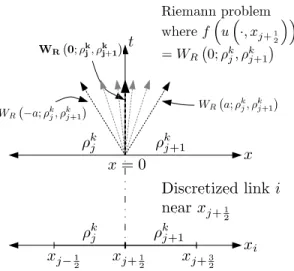
2.3 Godunov Discretization
In order to find approximate solutions we use the classical Godunov scheme [43]. We use the following notation: xj+1
2 are the cell interfaces and t
k
= k∆t the time with k 2 N and j 2 Z. xjis the center of the
cell, ∆x = xj+1 2− xj−
1
!" !"
Fig. 2: Space discretization for a link i 2 I. Step size is uniform ∆x, with discrete value ⇢k
j representing
the state between xj−1and xj.
Godunov scheme for a single link. The Godunov scheme is based on the solutions of exact Riemann prob-lems. The main idea of this method is to approximate the initial datum by a piecewise constant function, then the corresponding Riemann problems are solved exactly and a global solution is found by piecing them together. Finally one takes the mean on the cell and proceed by iteration. Given ⇢(t, x), the cell average of ⇢at time tkin the cell C
j=]xj−1 2, xj+ 1 2] is given by ⇢kj= 1 ∆x ˆ xj+ 1 2 xj− 1 2 ⇢(tk, x)dx. (6)
Then we proceed as follows:
1. We solve the Riemann problem at each cell interface xj+1
2 with initial data (⇢
k j, ⇢kj+1).
2. Compute the cell average at time tk+1in each computational cell and obtain ⇢k+1j .
We remark that waves in two neighbouring cells do not intersect before ∆t if the following Courant–Friedrichs–Lewy (CFL) condition holds, λmax∆x∆t, where λ
max= max
a |f 0
(a) | is the maximum wave speed of the Riemann solution at the interfaces.
Godunov scheme can be expressed as follows: ⇢k+1j = ⇢ k j− ∆t ∆x(g G (⇢kj, ⇢kj+1) − gG(⇢kj−1, ⇢kj)), (7)
where gGis the Godunov numerical flux given by
gG: R⇥ R ! R
#⇢j, ⇢j+1$ 7! gG#⇢j, ⇢j+1$ = f(WR(0; ⇢j, ⇢j+1)).
Godunov scheme at junctions. The scheme just discussed applies to the case in which a single cell is adjacent to another single cell. Yet, at junctions, a cell may share a boundary with more than one cell. A more general Godunov flux can be derived for such cases. For incoming links near the junction, we have:
⇢k+1L∆ i = ⇢ k L∆ i − ∆t ∆x(f (ˆ⇢ k L∆ i ) − g G (⇢kL∆ i−1, ⇢ k L∆ i )), i2 {1, . . . , n} where L∆
i are the number of cells for link i (see Fig. 2) and ˆ⇢ki is the solution of the Riemann solver
RS#⇢k
1, . . . , ⇢kn+m$ for link i at the junction. The same can be done for the outgoing links:
⇢k+11 = ⇢ k 1− ∆t ∆x(g G (⇢k1, ⇢k2) − f (ˆ⇢k1)), i2 {n + 1, . . . , n + m}
Remark 2 Using the Godunov scheme, each mesh grid at a given tk can be seen as a node for a 1-to-1
junction with one incoming and one outgoing link. It is therefore more convenient to consider that every discretized cell is, rather, a link with both an upstream and downstream junction. Thus, we consider networks in which the state of each link i 2 I at a time-step k 2 {0, . . . , T − 1} is represented by the single discrete value ⇢k
Fig. 3: Self-similar solution for Riemann problem with initial data#⇢k
j, ⇢kj+1$. The self-similar solution at x
t = 0 for the top diagram (i.e. WR#0; ⇢kj, ⇢kj+1$), gives the flux solution to the discretized problem in the
bottom diagram.
The previous remark allows us to develop a generalized update step for all discrete state variables. We first introduce a definition in order to reduce the cumbersome nature of the preceding notation. Let the state variables adjacent to a junction J 2 J at a time-step k 2 {0, . . . , T − 1} be represented as ρkJ := ⇣ ⇢ki1 J, . . . , ⇢ k inJ +mJJ ⌘
. Similarly, we let the solution of a Riemann solver be represented as ˆρJ :=
RS(ρJ). Then, for a link i 2 I with upstream and downstream junctions, J
U
i and J
D
i , and time-step
k2 {0, . . . , T − 1}, the update step becomes:
⇢k+1i = ⇢ k i− ∆t ∆x ⇣ f⇣⇣RS⇣ρkJD i ⌘⌘ i ⌘ − f⇣⇣RS⇣ρkJU i ⌘⌘ i ⌘⌘ = ⇢ki− ∆t ∆x ⇣ f⇣⇣ρˆ JD i ⌘ i ⌘ − f⇣⇣ρˆ JU i ⌘ i ⌘⌘ (8) where (s)iis the ith element of the tuple s. This equation is thus a general way of writing the Godunov
scheme in a way which applies everywhere, including at junctions.
Working directly with flux solutions at junctions. The equations can be simplified if we do not explicitly represent the solution of the Riemann solver, ˆρJ, and, instead, directly calculate the flux solution from the
Riemann data. We denote this direct computation by gG
J, the Godunov flux solution at a junction:
gJG: RnJ+mJ ! RnJ+mJ
ρJ 7! f (RS (ρJ)) = (f (ˆ⇢1) , . . . , f (ˆ⇢n+m)) . (9)
This gives a simplified expressions for the update step: ⇢k+1i = ⇢ k i − ∆t ∆x ⇣⇣ gGJD i ⇣ ρkJD i ⌘⌘ i− ⇣ gJGU i ⇣ ρkJU i ⌘⌘ i ⌘ . (10)
Full discrete solution method. We assume a discrete scalar hyperbolic network of PDEs with links I and junctions J , and a known discrete state at time-step k, # ¯⇢ki : i 2 I$. The solution method for advancing
Algorithm 1 Riemann solver update procedure Input: i n i t i a l s t a t e at time t= k∆t, !ρk i: i 2 I " Output: r e s u l t i n g s t a t e at time t= (k + 1)) ∆t, ⇣ρk+1i : i 2 I⌘ for j u n c t i o n J 2 J : # A p p l y R i e m a n n s o l v e r to J ˆ ρkJ= RS!ρkJ" for link i 2 I : # u p d a t e d e n s i t y on link i with j u n c t i o n f l u x e s ρk+1i = ρk i− ∆t ∆x ✓ f ✓✓ ˆ ρk JD i ◆ i ◆ − f ✓✓ ˆ ρk JU i ◆ i ◆◆
Algorithm 1 takes as input the state at a time-step k for all links#⇢k
i : i 2 I$ and returns the state
advanced by one time-step⇣⇢k+1i : i 2 I
⌘
. The algorithm first iterates over all junctions J, calculating all the boundary conditions, ˆρkJ. Then, the algorithm iterates over all links i 2 I to compute the updated state
⇢k+1i using the previously computed boundary conditions, as in 8.
Algorithm 2 Godunov junction flux update procedure
Input: i n i t i a l s t a t e at time t= k∆t, !ρk i: i 2 I " Output: r e s u l t i n g s t a t e at time t= (k + 1)) ∆t, ⇣ρk+1i : i 2 I⌘ for link i 2 I : # u p d a t e d e n s i t y on link i with d i r e c t G o d o n u v f l u x e s ρk+1i = ρk i− ∆t ∆x ✓✓ gG JD i ✓ ρk JD i ◆◆ i − ✓ gG JU i ✓ ρk JU i ◆◆ i ◆
Algorithm 2 is similar to Algorithm 1, except that the boundary conditions ˆρkJ are not explicitly
com-puted, but rather the Godunov flux solution is used to update the state, as in 10. Algorithm 2 is more suitable if a Godunov flux solution is derived for solving junctions, while Algorithm 1 is more suitable if one uses a Riemann solver at junctions.
2.4 State, Control, and Governing Equations
The rest of the article focuses on controlling systems of the form in Equation (10) in which some parts of the state can be controlled directly (for example, in the form of boundary control). We wish to solve the system in Algorithm 2 T time-steps forward, i.e. we wish to determine the discrete state values ⇢k
i for all links
i2 I and all time-steps k 2 {0, . . . , T − 1}. Furthermore, at each time-step k, we assume a set of “control” variables #uk
1, . . . , ukM$ 2 R M
that influence the solution of the Riemann problems at junctions, where M is the number of controlled values at each time-step, and each control may be updated at each time-step. We assume that a control may only influence a subset of junctions, which is a reasonable assumption if the controls have some spatial locality. Thus, for a junction J 2 J , we assume without loss of generality that a subset of the control parameters ⇣ukj1
J, . . . , u
k jJMJ
⌘
2 RMJ influence the solution of the Riemann solver.
Similar to the notation developed for state variables, for control variables, we define ukJ:=
⇣ ukj1 J, . . . , u k jJMJ ⌘
as the concatenation of the control variables around the junction J. To account for the addition of controls, we modify the Riemann problem at a junction J 2 J at time-step k to be a function of the current state of connecting links ρk
J, and the current control parameters ukJ. Then using the same notation as before, we
express the Riemann solver as:
RSJ : RnJ+mJ⇥ RMJ ! RnJ+mJ # ρkJ, u k J $ 7! RSJ ⇣ ρkJ, ukJ ⌘ = ˆρkJ.
We represent the entire state of the solved system with the vector ρ 2 RN T, where for i 2 I and
k 2 {0, . . . , T − 1}, we have ρN k+i = ⇢ki. Similarly, we represent the entire control vector by u 2 RM T,
where uM k+j= ukj.
For each state variable ⇢k
i, write the corresponding update equation hki:
hki : RN T⇥ RM T ! R
(ρ, u) 7! hki(ρ, u) = 0.
This takes the following form:
h0i(ρ, u) = ⇢0i − ¯⇢i= 0 (11) hki(ρ, u) = ⇢ k i − ⇢k−1i + ∆t Li f⇣RSJD i ⇣ ρk−1JD i , u k−1 JD i ⌘⌘ i −∆t Li f⇣RSJU i ⇣ ρk−1JU i , u k−1 JU i ⌘⌘ i= 0 8k 2 {2, . . . , T − 1} , (12)
or in terms of the Godunov junction flux:
hki(ρ, u) = ⇢ki − ⇢k−1i + ∆t ∆x ⇣ gJGD i ⇣ ρkJD i , u k−1 JD i ⌘⌘ i −∆t ∆x ⇣ gJGU i ⇣ ρkJU i , u k−1 JU i ⌘⌘ i (13)
for all links i 2 I, where ¯⇢i is the initial condition for link i. Thus, we can construct a system of N T
governing equations H (ρ, u) = 0, where the hi,k is the equation in H at index N k + i, identical to the
ordering of the corresponding discrete state variable.
3 Adjoint Based Flow Optimization 3.1 Optimal Control Problem Formulation
In addition to our governing equations H (ρ, u) = 0, we also introduce a cost function C, which we assume to be in C2:
C: RN T⇥ RM T ! R
(ρ, u) 7! C (ρ, u)
which returns a scalar that serves as a metric of performance of the state and control values of the system. We wish to minimize the quantity C over the set of control parameters u, while constraining the state of the system to satisfy the governing equations H (ρ, u) = 0, which is, again, the concatenated version of (12) or (13). We summarize this with the following optimization problem:
min
u
C(ρ, u)
subject to: H (ρ, u) = 0 (14)
3.2 Calculating the Gradient
We wish to use gradient information in order to find control values u⇤that give locally optimal costs C⇤=
C(ρ (u⇤) , u⇤). Since there may exist many local minima for this optimization problem (14) (which is
non-convex in general), gradient methods do not guarantee global optimality of u⇤. Still, nonlinear optimization
methods such as interior point optimization utilize gradient information to improve performance [46]. In a descent algorithm, the optimization procedure will have to descend a cost function, by coupling the gradient, which, at a nominal point#
ρ0, u0$ is given by: duC # ρ0, u0$ = @C(ρ, u) @ρ , , , , ρ0,u0 dρ du+ @C(ρ, u) @u , , , , ρ0,u0 . (15)
The main difficulty is to compute the term dudρ. Next we take advantage of the fact that the derivative
of H (ρ, u) with respect to u is equal to zero along trajectories of the system: duH # ρ0, u0$ = @H(ρ, u) @ρ , , , , ρ0,u0 dρ du+ @H(ρ, u) @u , , , , ρ0,u0 = 0. (16)
The partial derivative terms, Hρ2 R
N T ⇥N T, H u2 R N T ⇥M T, C ρ2 R N T, and C u2 R M T, can all be
evaluated (more details provided in Section 3.3) and then treated as constant matrices. Thus, in order to evaluate duC
#
ρ0, u0$ 2 RM T, we must solve a coupled system of matrix equations.
Note 1 In (16), Hρ and Hu might not necessarily be defined, either because f itself is not smooth (note
that we took f to be C2to avoid this problem), or because gGis not smooth. The derivations below are
valid when the partials Hρand Hucan indeed be taken. There are several settings in which the conditions
for differentiability are satisfied, see in particular [8, 47]. Forward system. If we solve for dρdu2 R
N T ⇥M T in (16), which we call the forward system:
Hρ
dρ
du= −Hu,
then we can substitute the solved value for dρ
du into (15) to obtain the full expression for the gradient.
Section 3.3 below gives details on the invertibility of Hρ, guaranteeing a solution for dρ du.
Adjoint system. Instead of evaluating dρdu directly, the adjoint method solves the following system, called
the adjoint system, for a new unknown variable λ 2 RN T (called the adjoint variable):
HρTλ= −C T
ρ (17)
Then the expression for the gradient becomes: duC
#
ρ0, u0$ = λTHu+ Cu (18)
We define Dρ to be the maximum junction degree on the network:
Dρ= max
J 2J(nJ+ mJ) , (19)
and also define Du to be the maximum number of constraints that a single control variable appears in,
which is equivalent to:
Du= max u2u X J 2J:u2uk J (nJ+ mJ) . (20) Note that-u 2 uk
J : J 2 J is a k-dependent set. By convention, junctions are either actuated or not,
so there is no dependency on k, i.e. if 9k s.t. u 2 uk
J, then 8k, u 2 ukJ.
Using these definitions, we show later in Section 3.4 how the complexity of computing the gradient is reduced from O(DρN M T2) to O(T (DρN+ DuM)) by considering the adjoint method over the forward
method.
A graphical depiction of Dρ and Duare given in Fig. 4. Freeway networks are usually considered to
! " # $ % & (a) ! " # $ % & (b) ! ! " # # $ $ % & (c)
Fig. 4: Depiction of Dρand Dvfor an arbitrary graph. Fig. 4a shows the underlying graphical structure
for an arbitrary PDE network. Some control parameter u1has influence over junctions A, B, and F , while
another control parameter u2has influence over only junction C. Fig. 4b depicts the center junction having
the largest number of connecting edges, thus giving Dρ = 5. Fig. 4c shows that control parameter u1
influences three junctions with sum of junctions degrees equal to six, which is maximal over the other control parameter u2. leading to the result Du= 6. Note that in Fig. 4c, the link going from junction A to
junction B is counted twice: once as an outgoing link AB and once as in incoming link BA.
regardless of the total number of links. Also, from the locality argument for control variables in Section (2.4), a single control variable’s influence over state variables will not grow with the size of the network. Since the Dρand Dutypically do not grow with N T or M T for freeway networks, the complexity of evaluating
the gradient for such networks can be considered linear for the adjoint method.
3.3 Evaluating the Partial Derivatives
While no assumptions are made about the sparsity of the cost function C, the networked-structure of the PDE system and the Godunov discretization scheme allows us to say more about the structure and sparsity of Hρ and Hu.
Partial derivative expressions. Given that the governing equations require the evaluation of a Riemann solver at each step, we detail some of the necessary computational steps in evaluating the Hρ and Hu
matrices.
If we consider a particular governing equation hk
i(ρ, u) = 0, then we may determine the partial term
with respect to ⇢l
j2 ρ by applying the chain rule:
@hki @⇢l j =@⇢ k i @⇢l j −@⇢ k−1 i @⇢l j +∆t Li f0⇣RSJD i ⇣ ρk−1JD i , uk−1JD i ⌘ i ⌘ @ @⇢l j ⇣ RSJD i ⇣ ρk−1JD i , uk−1JD i ⌘ i ⌘ (21) −∆t Li f0⇣RSJU i ⇣ ρk−1JU i , u k−1 JU i ⌘ i ⌘ @ @⇢l j ⇣ RSJU i ⇣ ρk−1JU i , u k−1 JU i ⌘ i ⌘
or if we consider the composed Riemann flux solver gG J in (9): @hki @⇢l j = @⇢ k i @⇢l j −@⇢ k−1 i @⇢l j +∆t Li @ @⇢l j ⇣ gJGD i ⇣ ρk−1JD i , u k−1 JD i ⌘⌘ i− @ @⇢l j ⇣ gJGU i ⇣ ρk−1JU i , u k−1 JU i ⌘⌘ i ! (22) A diagram of the structure of the Hρ matrix is given in Fig. (5a). Similarly for Hu, we take a control
parameter ul
j2 u, and derive the expression:
@hki @ul j = +∆t Li f0⇣RSJD i ⇣ ρk−1JD i , u k−1 JD i ⌘ i ⌘ @ @ul j ⇣ RSJD i ⇣ ρk−1JD i , u k−1 JD i ⌘ i ⌘ (23) −∆t Li f0⇣RSJU i ⇣ ρk−1JU i , u k−1 JU i ⌘ i ⌘ @ @ul j ⇣ RSJU i ⇣ ρk−1JU i , u k−1 JU i ⌘ i ⌘
or for the composed Godunov junction flux solver gG J:
(a) Ordering of the partial derivative terms. Constraints and state variables are clustered first by time, and then by cell index.
(b) Sparsity structure of the Hρmatrix. Besides the di-agonal blocks, which are identity matrices, blocks where l 6= k − 1 are zero.
Fig. 5: Structure of the Hρ matrix.
@hki @ul j =∆t Li @ @ul j ⇣ gGJD i ⇣ ρk−1JD i , u k−1 JD i ⌘⌘ i− @ @ul j ⇣ gJGU i ⇣ ρk−1JU i , u k−1 JU i ⌘⌘ i ! . (24)
Analyzing (21), the only partial terms that are not trivial to compute are ∂ ∂ρl j ⇣ RSJD i ⇣ ρk−1JD i , uk−1JD i ⌘ i ⌘ and ∂ ∂ρl j ⇣ RSJU i ⇣ ρk−1JU i , u k−1 JU i ⌘ i ⌘
. Similarly for (23), the only nontrivial terms are ∂ ∂ul j ⇣ RSJD i ⇣ ρk−1JD i , u k−1 JD i ⌘ i ⌘ and ∂ ∂ul j ⇣ RSJU i ⇣ ρk−1JU i , uk−1JU i ⌘ i ⌘
. Once one obtains the solutions to these partial terms, then one can con-struct the full Hρand Humatrices and use (17) and (18) to obtain the gradient value.
As these expressions are written for a general scalar conservation law, the only steps in computing the gradient that are specific to a particular conservation law and Riemann solver are computing the derivative of the flux function f and the partial derivative terms just discussed. These expressions are explicitly calculated for the problem of optimal ramp metering in Section (4).
3.4 Complexity of Solving Gradient via Forward Method vs. Adjoint Method This section demostrates the following proposition:
Proposition 31 The total complexity for the adjoint method on a scalar hyperbolic network of PDEs is
O(T (DρN+ DuM)).
We can show the lower-triangular structure and invertibility of Hρ by examining (11) and (12). For
k2 {1, . . . , T − 1}, we have that hki is only a function of ⇢ k
i and of the state variables from the previous
time-step k − 1. Thus, based on our ordering scheme in Section 2.4 of ordering variables by increasing time-step and ordering constraints by corresponding variable, we know that the diagonal terms of Hρ are
always 1 and all upper-triangular terms must be zero (since those terms correspond to constraints with a dependence of future values). These two conditions demonstrate both that Hρ is lower-triangular and is
invertible due to the ones along the diagonal.
Additionally, if we consider taking partial derivatives with respect to the variable ⇢l
j, then we can
deduce from Equation (12) that all partial terms will be zero except for the diagonal term, and those terms involving constraints at time j + 1 with links connecting to the downstream and upstream junctions JjD and J
U
Fig. 6: Freeway network model. For a junction JD
2i−1= J2(i−1)D = J U
2iat time-step k 2 {0, . . . , T − 1}, the
upstream mainline density are represented by ⇢k2(i−1), the downstream mainline density by ⇢ k
2i, the on-ramp
density by ⇢k
2i−1, and the off-ramp split ratio by βk2(i−1).
invertible, lower-triangular and each column will have a maximum cardinality equal to Dρ in (19). The
sparsity structure of Hρis depicted in Fig. 5b.
Using the same line of argument for the maximum cardinality of Hρ, we can bound the maximum
cardinality of each column of Hu. Taking a single control variable u l
j, the variable can only appear in the
constraints at time-step j + 1 that correspond to a link that connects to a junction J such that ul j2 ul+1J .
These conditions give us the expression for Duin (20), or the maximum cardinality over all columns in Hu.
If we only consider the lower triangular form of Hρ, then the complexity of solving for the gradient using
the forward system is O((N T )2M T), where the dominating term comes from solving (15), which requires the solution of M T separate N T ⇥ N T lower-triangular systems. The lower-triangular system allows for forward substitution, which can be solved in O((N T )2) steps, giving the overall complexity O((N T )2M T).
The complexity of computing the gradient via the adjoint method is O((N T )2+ (N T ) (M T )), which
is certainly more efficient than the forward-method, as long as M T > 1. The efficiency is gained by considering that (17) only requires the solution of a single N T ⇥N T upper -triangular system (via backward-substitution), followed by the multiplication of λT
Hv, an N T ⇥ N T and an N T ⇥ M T matrix in (18), with
a complexity of O((N T )2+ (N T ) (M T )).
For the adjoint method, this complexity can be improved upon by considering the sparsity of the Hρ
and Humatrices, as detailed in Section 3.4. For the backward-substitution step, each entry in the λ vector
is solved by at most Dρ multiplications, and thus the complexity of solving (17) is reduced to O(DρN T).
Similarly, for the matrix multiplication of λTHv, while λ is not necessarily sparse, we know that each entry
in the resulting vector requires at most Dumultiplications, giving a complexity of O(DuM T).
4 Applications to Optimal Coordinated Ramp Metering on Freeways 4.1 Formulation of the Network Model And Explicit Riemann Solver
Model. Consider a freeway section with links I = {1, . . . , 2N } with a linear sequence of mainline links = {2, 4, . . . , 2N } and connecting on-ramp links = {1, 3, . . . , 2N − 1}. At discrete time t = k∆t, 0 k T − 1, mainline link 2i 2 I, i 2 {1, . . . , N } has a downstream junction JD
2i = J U
2(i+1) and an upstream junction
JU
2i= J2(i−1)D , while on-ramp 2i − 1 2 I, i 2 {1, . . . , N } has a downstream junction J D
2i−1= J2iU = J2(i−1)D
and an upstream junction JU 2i−1.
The off-ramp directly downstream of link 2i, i 2 {1, . . . , N } has, at time-step k, a split ratio βk 2i
rep-resenting the ratio of cars which stay on the freeway over the total cars leaving the upstream mainline of junction JD
2i. The model assumes that all flux from on-ramp 2i − 1 enters downstream mainline 2i. Since J U 2
is the source of the network, it has no upstream mainline or off-ramp, and similarly JD
2Nhas no downstream
mainline or on-ramp (βk2N = 0). Each link i 2 I has a discretized state value ⇢ki 2 R at each time-step
k2 {0, . . . , T − 1}, that represents the density of vehicles on the link. These values are depicted in Fig. 6. Junctions that have no on-ramps can be effectively represented by adding an on-ramp with no demand while junctions with no off-ramps can be represented by setting the split ratio to 1.
The vehicle flow dynamics on all links i (mainlines, on-ramps, and off-ramps) are modeled using the conservation law governing the density evolution (1), where ⇢ is the density state, and f is the flux function (or fundamental diagram) f (⇢). In the context of traffic, this model is referred to as the Lighthill-Whitham-Richards (LWR) model [36, 35]. The fundamental diagram f is typically assumed to be concave, and has a bounded domain [0, ⇢max] and a maximum flux value Fmaxattained at a critical density ⇢c: f (⇢c) = Fmax. We assume that the fundamental diagram has a trapezoidal form as depicted in Fig. 7. For the remainder of
the article, we instantiate the conservation law in (1) with the LWR equation as it applies to traffic flow mod-eling.
Fig. 7: Fundamental diagram (the name of the flux function in transportation literature) with free-flow
speed v, congestion wave speed w, max flux Fmax,
critical density ⇢c, and max density ⇢max. As control input, an on-ramp 2i − 1 2 I, i 2
{1, . . . , N } at time-step k 2 {0, . . . , T − 1} has a metering rate uk
2i−12 [0, 1] which limits the flux
of vehicles leaving the on-ramp. Intuitively, the metering rate acts as a fractional decrease in the flow leaving the on-ramp and entering the main-line freeway. The domain of the metering control is to force the control to neither impose nega-tive flows nor send more vehicles than present in a queue. Its mathematical model is expressed in (31).
For notational simplicity we define the set of densities of links incident to JU
2i = J2(i−1)D at time-step k as ρkJU 2i = n ⇢k2(i−1), ⇢k2i−1, ⇢k2i o . The off-ramp is considered to have infinite capacity, and thus has no bearing on the solution of junc-tion problems. Initial condijunc-tions are handled as
in (11), while for k 2 {1, . . . , T − 1}, the mainline density ⇢k
2iusing the Godunov scheme from (12) is given
by: hk2i(ρ, u) = ⇢k2i− ⇢k−12i + ∆t L2i ⇣ gGJD 2i ⇣ ρk−1JD 2i , u k−1 2i+1 ⌘⌘ 2i (25) −∆t L2i ⇣ gGJU 2i ⇣ ρk−1JU 2i , u k−1 2i−1 ⌘⌘ 2i = ⇢k 2i− ⇢k−12i + ∆t L2i ⇣ gk−12i,D− g2i,Uk−1 ⌘ = 0 (26)
where we have introduced some substitutions to reduce the notational burden of this section: gk i,Dis the
Godunov flux at time-step k exiting a link i at the downstream boundary of the link, and gk
i,U is the
Godunov flux entering the link at the upstream boundary.
We also make the assumption that on-ramps have infinite capacity and a free-flow velocity v2i−1=L∆t2i−1
to prevent the ramp congestion from blocking demand from ever entering the network. Since the on-ramp has no physical length, the length is chosen arbitrarily and the “virtual” velocity chosen above is chosen to replicate the dynamics in [48]. We can then simplify the on-ramp update equation to be:
hk2i−1(ρ, u) = ⇢k2i−1− ⇢k−12i−1−
∆t L2i−1 ✓ ⇣ gGJU 2i ⇣ ρk−1JU 2i , u k−1 2i−1 ⌘⌘ 2i−1− D k−1 2i−1 ◆ (27) = ⇢k2i−1− ⇢k−12i−1− ∆t L2i−1 ⇣ gk−12i−1,D− Dk−12i−1 ⌘ = 0 (28)
where Dk−12i−1is the on-ramp flux demand, and the same notational simplification has been used for the
downstream flux. This formulation results in “strong” boundary conditions at the on-ramps which guarantees all demand enters the network. Details on weak versus strong boundary conditions can be found in [48, 22, 6].
The on-ramp model in (27) differs from [48] in that we model the on-ramp as a discretized PDE with an infinite critical density, while [48] models the on-ramp as an ODE “buffer”. While both models implement strong boundary conditions, the discretized PDE model makes the freeway network more aligned with the PDE network framework presented in this article.
Riemann solver. For the ramp metering problem, there are many potential Riemann solvers that satisfy the properties required in Section 2.2. Following the model of [48], for each junction JU
2i, we add two modeling
decisions:
1. The flux solution maximizes the outgoing mainline flux gk 2i,U.
(a) Case 1: Priority violated due to limited upstream mainline demand entering downstream mainline.
(b) Case 2: Priority violated due to limited on-ramp demand entering downstream mainline.
(c) Case 3: Priority rule satisfied due to sufficient demand from both main-line and on-ramp.
Fig. 8: Godunov junction flux solution for ramp metering model at junction JU
2i. The rectangular region
represents the feasible flux values for β2(i−1)g2(i−1),D and g2i−1,D as determined by the upstream
de-mand, while the line with slope 1
β2(i−1) represents feasible flux values as determined by mass balance. The
β2(i−1)g2(i−1),D term accounts for only the flux out of link 2 (i − 1) that stays on the mainline. The flux
solution, represented by the red circle, is the point on the feasible region that minimizes the distance from the priority line β2(i−1)g2(i−1),D= p2(i−1)g2i−1,D.
2. Subject to (1), the flux solution attempts to satisfy g2(i−1),Dk = p2(i−1)gk2i−1,D, where p2(i−1)2 R+is a
merging parameter for junction JD
2(i−1). Since (1) allows multiple flux solutions at the junction, (2) is
necessary to obtain a unique solution.
This leads to the following system of equations that gives the flux solution of the Riemann solver at time-step k2 {1, . . . , T − 1} and junction JU
2ifor i 2 {1, . . . , N }:
δ2(i−1)k = min
⇣
v2(i−1)⇢k2(i−1), F2(i−1)max
⌘ (29) σk2i= min ⇣ w2i ⇣ ⇢max2i − ⇢k2i ⌘ , F2imax ⌘ (30) dk2i−1= uk2i−1min
✓ L2i−1
∆t ⇢
k
2i−1, F2i−1max
◆ (31) g2i,Uk = min ⇣ β2(i−1)k δ k 2(i−1)+ d k 2i−1, σk2i ⌘ (32) g2(i−1),Dk = 8 > > > > < > > > > :
δk2(i−1) p2(i−1)g2i,Uk
βk 2(i−1)(1+p2(i−1))≥ δ k 2(i−1)[Case 1] gk 2i,U−d k 2i−1 βk 2(i−1) gk 2i,U 1+p2(i−1) ≥ d k 2i−1 [Case 2] p2(i−1)gk2i,U (1+p2(i−1))βk2(i−1) otherwise [Case 3] (33)
g2i−1,Dk = gk2i,U− β2(i−1)k g k
2(i−1),D (34)
where, for notational simplicity, at the edges of of the range for i, any undefined state values (e.g. ⇢k0) are
assumed to be zero by convention. Equations (29) and (31) determine the maximum flux that can exit link 2(i − 1) and link 2i − 1 respectively. Equation (30) gives the maximum flux allowed into link 2i. The actual flux into link 2i, shown in (32), is given as the minimum of the “demand” from upstream links and “supply” of the downstream link. See [48] for more details on the model for this equation. The flux out of link 2(i − 1) is split into three cases in (33). The solutions are depicted in Fig. 8, which demonstrates how the flux solution depends upon the respective demands and the merging parameter p2(i−1). Finally,
Equation (34) gives the flux out of the on-ramp 2i − 1, which is the difference between the flux into link 2i and the flux out of link 2 (i − 1) the remains on the mainline.
For k = 0, the update equation is given by a pre-specified initial condition, as in (11). Note that the equations can be solved sequentially via forward substitution. Also, we do not include the flux result for off-ramps explicitly here since its value has no bearing on further calculations, and we will henceforth ignore its calculation. To demonstrate that indeed the flux solution satisfies the flux conservation property, the off-ramp flux is trivially determined to be βk
4.2 Formulation of the Optimal Control Problem
Optimal coordinated ramp-metering. Including the initial conditions as specified in (11) with (25) and (27) gives a complete description of the system H (ρ, u) = 0, ρ 2 R2N, u 2 R, where:
ρ2N k+i:= ⇢ki 1 i 2N, 0 k T − 1
uN k+i:= uk2i1 i N, 0 k T − 1
The objective of the control is to minimize the total travel time on the network, expressed by the cost function C: C(ρ, u) = ∆t T X k=1 2N X i=1 Li⇢ki.
The optimal coordinated ramp-metering problem can be formulated as an optimization problem with PDE-network constraints: min u C(ρ, u) (35) subject to: H (ρ, u) = 0 0 u 1 8u 2 u
Since the adjoint method in Section 3 only deals with equality constraints, we add barrier penalties to the cost function [49, 9]:
˜
C(ρ, u, ✏) = C (ρ, u) − ✏X
u2u
log ((1 − u) (u − 0)) . (36)
As ✏ 2 R+ tends to zero, the solution to (36) will approach the solution to the original problem (35).
Thus we can solve (35) by iteratively solving the augmented problem:
min
u
˜
C(ρ, u, ✏) (37)
subject to: H (ρ, u) = 0
with decreasing values of ✏. As a result, ˜Cwill approach C as the number of iterations increases.
Applying the adjoint method. To use the adjoint method as described in Section 3, we need to compute the partial derivative matrices Hρ, Hu, ˜Cρand ˜Cu. Computing the partial derivatives with respect to the cost
function is straight forward:
@ ˜C @⇢k i = ∆tLi 1 i 2N, 0 k T − 1 @ ˜C @uk 2i = ✏⇣1−u1k 2i− 1 uk 2i ⌘ 1 i N, 0 k T − 1
To compute the partial derivatives of H, we follow the procedure in Section 3.2. For an upstream junction JU
2i2 J and time-step k 2 {1, . . . , T − 1}, we only need to compute the partial derivatives of the
flux solver gGJU 2i ⇣ ρkJU 2i, u k 2i−1 ⌘
with respect to the adjacent state variables ρkJiand ramp metering control u
k i.
We calculate the partial derivatives of the functions in (29)-(34) with respect to either a state or control variables 2 ρ [ u:
@δk 2(i−1)
@s =
(
v2(i−1) s= ⇢k2(i−1), vi⇢k2(i−1) F2(i−1)max
0 otherwise @σk2i @s = ( −w2i s= ⇢k2i, w2i#⇢max2i − ⇢k2i$ F2imax 0 otherwise @d @s = 8 > < > :
uk2i−1 s= ⇢k2i−1, ⇢k2i−1 F2i−1max
min#⇢k
2i−1, F2i−1max$ s= uk2i−1
0 otherwise @ @sg k 2i,U= 8 < : βk 2(i−1) ∂δk 2(i−1) ∂s + ∂dk 2(i−1) ∂s β k
2(i−1)δk2(i−1)+ dk2i−1 σ2ik ∂σk 2i ∂s otherwise @ @sg2(i−1),D= 8 > > > > < > > > > : ∂δk 2(i−1) ∂s gk 2i,Up2(i−1) 1+p2(i−1) ≥ δk 2(i−1) βk 2(i−1) 1 βk 2(i−1) ✓ ∂ ∂sg k 2i,U− ∂dk 2i−1 ∂s ◆ gk 2i,U 1+p2(i−1) ≥ d k 2(i−1) p2(i−1) βk 2(i−1)(1+p2(i−1)) ∂ ∂sg k 2i,U otherwise @ @sg2i−1,D = @ @sg k 2i,U− βk2(i−1) @ @sg2(i−1),D
These expressions fully quantify the partial derivative values needed in (22) and (24). Thus we can construct the Hρ and Hu matrices. With these matrices and Cρ and Cu, we can solve for the adjoint
variable λ 2 R2N T in (17) and substitute its value into (18) to obtain the gradient of the cost function C with respect to the control parameter u.
5 Numerical Results for Model Predictive Control Implementations
To demonstrate the effectiveness of using the adjoint ramp metering method to compute gradients, we implemented the algorithm on practical scenarios with field experimental data. The algorithm can then be used as a gradient computation subroutine inside any descent-method optimization solver that takes advantage of first-order gradient information. Our implementation makes use of the open-source IpOpt solver [46], an interior point, nonlinear program optimizer. To serve as comparisons, two other case scenarios were run:
1. No control: the metering rate is set to 1 on all on-ramps at all times.
2. Alinea [38]: a well-adopted, feedback-based ramp metering algorithm commonly used in the practi-tioner’s community. Alinea is computationally efficient and decentralized, making it a popular choice for large networks, but does not take estimated boundary flow data as input. Since Alinea has a number of tuning parameters, we perform a modified grid-search technique over the different parameters that scales linearly with the number of on-ramps, and select the best-performing parameters, in order to be fair to this framework. A full grid-search approach scales exponentially with the number of on-ramps, rendering it infeasible for moderate-size freeway networks.
All simulations were run on a 2012 commercial laptop with 8 GB of RAM and a dual-core 1.8 GHz Intel Core i5 processor.
Note 2 To demonstrate the reduced running time associated with the adjoint approach, we also imple-mented a gradient descent using a finite differences approach similar to [33, 32], which requires an O(T2N M)
computation for each step in gradient descent, but it proved to be computationally infeasible for even small, synthetic networks. Running ramp metering on even a network of 4 links over 6 time-steps for 5 gradient steps took well over 4 minutes, rendering the method useless for real-time applications. The comparison of running times of finite differences versus the adjoint method is given in Fig. 9. Due to the impractically large running times associated with finite differences, we do not consider the finite differences in further results, which only becomes worse as the problem scales to larger networks and time horizons.
10−1 100 101 102 103 Running time(ms) 226 227 228 229 230 231 232 233 234 T ot al tr av el ti m e (v eh-s) Finite differences Adjoint
Fig. 9: Running time of ramp metering algorithm using IpOpt with and without gradient information. Network consists of 4 links and 6 time-steps with synthetic boundary flux data. The method using gradient information via the adjoint method converged well before the completion of the first step of the finite differences descent method.
Fig. 10: Model of section of I15 South in San Diego, California. The freeway section spanning 19.4 miles was split into 125 links with 9 on-ramps.
5.1 Implementation of I15S in San Diego
As input into the optimization problem, we constructed a model of a 19.4 mile stretch of the I15 South freeway in San Diego, California between San Marcos and Mira Mesa. The network has N = 125 links, and M= 9 on-ramps, with boundary data specified for T = 1800 time-steps, for a time horizon of 120 minutes given ∆t =4 seconds. The network is shown in Fig. 10.
Link length data was obtained using the Scenario Editor software developed as part of the Connected Corridors project, a collaboration between UC Berkeley and PATH research institute in Berkeley, Califor-nia. Fundamental diagram parameters, split ratios, and boundary data were also obtained using calibration techniques developed by Connected Corridors. Densities resulting in free-flow speeds were chosen as ini-tial conditions on the mainline and on-ramps. The data used in calibration was taken from PeMS sensor data [50] during a morning rush hour period, scaled to generate congested conditions. The input data was chosen to demonstrate the effectiveness of the adjoint ramp metering method in a real-world setting. A profile of the mainline and on-ramps during a forward-simulation of the network is shown in Fig. 11 under the described boundary conditions.
5.2 Finite-Horizon Optimal Control
Experimental Setup. The adjoint ramp metering algorithm is compared to the reactive Alinea scheme, for which we assume that perfect boundary conditions and initial conditions are available. The metric we use to compare the different strategies is reduced-congestion percentage, ¯c2 (−1, 100], which we define as:
¯ c= 100 ✓ 1 − cc cnc ◆
where cc, cnc 2 R+ are the congestion resulting from the control and no-control scenarios, respectively.
We use the metric for congestion as defined in [51]; for a given section of road S and time horizon T , the congestion is given as c(S, T ) = X (s2S,τ 2T ) max TTT (s, ⌧ ) −VMT (s, ⌧ ) vs ,0 6
(a) Density profile. The units are the ratio of a link’s vehicle density to a link’s jam density.
(b) On-ramp queue profile in units of vehicles.
Fig. 11: Density and queue profile of no-control freeway simulation. In the first 80 minutes, congestion pockets form on the freeway and queues form on the on-ramps, then eventually clear out before 120 minutes.
(a) Density difference profile in units of change in density from the control scenario to the no control scenario over the jam density of the link.
(b) Queue difference profile in units of vehicles.
Fig. 12: Profile differences for mainline densities and on-ramp queues. Evidenced by the mainly negative differences in the mainline densities and the mainly positive differences in the on-ramp queue lengths, the adjoint ramp metering algorithm effectively limits on-ramp flows in order to reduce mainly congestion. View in color.
where vs is the free-flow velocity, VMT is total vehicle miles traveled, and TTT is total travel time over
the link s and time-step ⌧ . Since it is infeasible to compute the global optimum for all cases, a reduced congestion of 100% serves as an upper bound on the possible amount of improvement.
Results. Fig. 12 shows a difference profile for both density and queue lengths between the no control simulation and the simulation applying the ramp metering policy generated from the adjoint method. Negative differences in Figs. 12a and 12b indicate where the adjoint method resulted in fewer vehicles for the specific link and time-step. The adjoint method was successful in appropriately deciding which ramps should be metered in order to improve throughput for the mainline.
Running time analysis shows that the adjoint method can produce beneficial results in real-time appli-cations. Fig. 13 details the improvement of the adjoint method as a function of the overall running time of the algorithm. After just a few gradient steps, the adjoint method outperforms the Alinea method. Given that the time horizon of two hours is longer than the period of time one can expect reasonably accurate boundary flow estimates, more practical simulations with shorter time horizons should permit more gradient steps in a real-time setting.
While the adjoint method leads to queues with a considerable number of cars in some on-ramps, this can be addressed by introducing barrier terms into the cost function that limit the maximum queue length. The Alinea method tested for the I15 network had no prescribed maximum queue lengths as well, but was
0 50 100 150 200 250 300 350 400 450
Running time(seconds)
0.0 0.5 1.0 1.5 2.0 2.5 3.0 3.5 R educ ed C onge st ion (%) Adjoint Alinea
Fig. 13: Reduced congestion versus simulation time for freeway network. The results indicate that the algorithm can run with performance better than Alinea if given an update time of less than a minute.
not able to produce significant improvements in total travel time reduction, while the adjoint method was more successful.
5.3 Model Predictive Control
To study the performance of the algorithm under noisy input data, we embed both our adjoint ramp metering algorithm and the Alinea algorithm inside of a model predictive control (MPC) loop.
Experimental Setup. The MPC loop begins at a time t by estimating the initial conditions of the traffic on the freeway network and the predicted boundary fluxes over a certain time horizon Th. These values
are noisy, as exact estimation of these parameters is not possible on real freeway networks. The estimated conditions are then passed to the ramp metering algorithm to compute an optimal control policy over the Thtime period. The system is then forward-simulated over an update period of Tu Th, using the
exact initial conditions and boundary conditions, as opposed to the noisy data used to compute control parameters. The state of the system and boundary conditions at t + Tuare then estimated (with noise)
and the process is repeated.
A non-negative noise factor, σ 2 R+, is used to study how the adjoint method and Alinea perform as
the quality of estimated data decreases. If ⇢ is the actual density for a cell and time-step, then the density ¯
⇢passed to the control schemes is given by: ¯
⇢= ⇢ · (1 + σ · R)
where R is a uniformly distributed random variable with mean 0 and domain [−0.5, 0.5]. The noise factor was applied to both initial and boundary conditions.
Two different experiments were conducted:
1. Real-time I15 South: MPC is run for the I15 South network with Th= 80 minutes and Tu = 26
minutes. A noise factor of 2% was chosen for the initial and boundary conditions. The number of iterations was chosen in order to ensure that each MPC iteration finished in the predetermined update time Tu.
2. Noise Robustness: MPC is for over a synthetic network with length 12 miles and boundary conditions over 75 minutes. The experiments are run over a profile of noise factors between 1% and 8000%. Results. Real-Time I15 South. The results are summarized in Fig. 14a. The adjoint method applied once to the entire horizon with perfect boundary and initial condition information serves as a baseline performance for the other simulations, which had noisy input data and limited knowledge of predicted boundary conditions. The adjoint method still performs well under the more realistic conditions of the MPC loop with noise, resulting in 2% reduced congestion or 40 car-hours in relation to no control, as compared to the 3% reduced (60 car-hours) congestion achieved by the adjoint method with no noise and
full time horizon (Th = T ). In comparison, the Alinea method was only able to achieve 1.5% reduced
congestion (30 car-hours) for both the noisy and no-noise scenarios. The results indicate that, under a realistic assumption of a 2% noise factor in the sensor information, the algorithm’s ability to consider boundary conditions results in an improvement upon strictly reactive policies, such as Alinea.
Adjoint Adjoint w/ Noise Alinea Alinea w/ Noise 0.0 0.5 1.0 1.5 2.0 2.5 3.0 3.5 R educ ed C onge st ion (%)
(a) Reduced congestion.
10−2 10−1 100 101 102 Noise factor(-) 0.0 0.5 1.0 1.5 2.0 2.5 3.0 3.5 4.0 R educ ed C onge st ion (%) Adjoint Alinea
(b) Reduced congestion with increasing sensor noise for network with synthetic data.
Fig. 14: Summary of model predictive control simulations. The results indicate that the adjoint method has superior performance for moderate noise levels on the initial and boundary conditions.
Robustness to Noise.Simulation results on the synthetic network with varying levels of noise are
shown in Fig. 14b. The adjoint method is able to outperform the Alinea method when the noise level is less than 80%, a reasonable assumption for data provided by well-maintained loop detectors. As the initial and boundary condition data deteriorates, the adjoint method becomes useless. Since Alinea does not rely on boundary data, it is able to produce improvements, even with severely noisy data. The results indicate that the adjoint method will outperform Alinea under reasonable noise levels in the sensor data.
6 Conclusions
This article has detailed a simple framework for finite-horizon optimal control methods on a network of scalar conservation laws derived from first discretizing the network via the Godunov method, then applying the discrete adjoint to this system. To tailor the framework to a specific application, one need only provide the partial derivatives of the Riemann solver at a network junction as well as the partial derivatives of the objective. Furthermore, we show that for this class of problems, the sparsity pattern allows the problem to be implemented with only linear memory and linear computational complexity with respect to the number of state and control parameters. We demonstrate the scalability of the approach by implementing a coordinated ramp metering algorithm using the adjoint method and applying the algorithm to the I-15 South freeway in California. The algorithm runs in a fraction of real-time and produces significant improvements over existing algorithms. The ramp metering algorithm has been fully implemented within Connected Corridors [52] system, a project by UC Berkeley and PATH for integrated corridor management, as a component of the traffic simulator module. Future work includes investigating decentralized, coordinated control schemes over physical networks via the adjoint method to allow traffic control strategies to scale to regional-scale networks.
7 Acknowledgments
The authors have been supported by the California Department of Transportation under the Connected Corridors program, CAREER grant CNS-0845076 under the project ’Lagrangian Sensing in Large Scale Cyber-Physical Infrastructure Systems’, the European Research Council under the European Union’s Sev-enth Framework Program (FP/2007-2013) / ERC Grant Agreement n. 257661, the INRIA associated team ’Optimal REroute Strategies for Traffic managEment’ and the France-Berkeley Fund under the project ’Optimal Traffic Flow Management with GPS Enabled Smartphones’.
References
[1] B. Rothfarb et al. “Optimal design of offshore natural-gas pipeline systems”. In: Operations Research 18.6 (1970), pp. 992–1020.
[2] S. Brunnermeier and S. Martin. Interoperability cost analysis of the US automotive supply chain: Final report. Tech. rep. DIANE Publishing, 1999.
[3] T. S. Rabbani et al. “Feed-Forward Control of Open Channel Flow Using Differential Flatness”. In: IEEE Transactions on Control Systems Technology 18.1 (Jan. 2010), pp. 213–221. issn: 1063-6536.
doi: 10.1109/TCST.2009.2014640.
[4] X. Litrico and V. Fromion. “Boundary control of hyperbolic conservation laws using a frequency
domain approach”. In: Automatica 45.3 (2009), pp. 647–656.
[5] M. Garavello and B. Piccoli. Traffic flow on networks. Vol. 1. American institute of mathematical sciences Springfield, MA, USA, 2006. isbn: 9781601330000.
[6] D. B. Work et al. “A traffic model for velocity data assimilation”. In: Applied Mathematics Research eXpress 2010.1 (Apr. 2010), p. 1. issn: 1687-1200. doi: 10.1093/amrx/abq002.
[7] E. Frazzoli, M. A. Dahleh, and E. Feron. “Real-time motion planning for agile autonomous vehicles”. In: Journal of Guidance, Control, and Dynamics 25.1 (2002), pp. 116–129.
[8] M. Gugat et al. “Optimal Control for Traffic Flow Networks”. In: Journal of Optimization Theory and Applications 126.3 (Sept. 2005), pp. 589–616. issn: 0022-3239. doi: 10.1007/s10957-005-5499-z. [9] A. Bayen, R. Raffard, and C. Tomlin. “Adjoint-based control of a new eulerian network model of air
traffic flow”. In: IEEE Transactions on Control Systems Technology 14.5 (Sept. 2006), pp. 804–818.
issn: 1063-6536. doi: 10.1109/TCST.2006.876904.
[10] A. Kotsialos and M. Papageorgiou. “Nonlinear Optimal Control Applied to Coordinated Ramp
Me-tering”. In: IEEE Transactions on Control Systems Technology 12.6 (Nov. 2004), pp. 920–933. issn: 1063-6536. doi: 10.1109/TCST.2004.833406.
[11] J.-M. Coron et al. “Local Exponential H 2 Stabilization of a 2 X 2 Quasilinear Hyperbolic System
Using Backstepping”. In: SIAM Journal on Control and Optimization 51.3 (2013), pp. 2005–2035.
issn: 07431546. doi: 10.1109/CDC.2011.6161075.
[12] O. Glass and S. Guerrero. “On the uniform controllability of the Burgers equation”. In: SIAM Jour-nal on Control and Optimization 46.4 (Jan. 2007), pp. 1211–1238. issn: 0363-0129. doi: 10.1137/ 060664677.
[13] D. Jacquet, M. Krstic, and C. C. de Wit. “Optimal control of scalar one-dimensional conservation
laws”. In: American Control Conference, 2006. 2. IEEE. Ieee, 2006, 6–pp. isbn: 1-4244-0209-3. doi: 10.1109/ACC.2006.1657550.
[14] L. Blanchard et al. “Shape Gradient for Isogeometric Structural Design”. In: Journal of Optimization Theory and Applications (Sept. 2013), pp. 1–7. issn: 0022-3239. doi: 10.1007/s10957-013-0435-0. [15] D. Keller. “Optimal Control of a Nonlinear Stochastic Schrodinger Equation”. In: Journal of
Opti-mization Theory and Applications (Sept. 2013). issn: 0022-3239. doi: 10.1007/s10957-013-0399-0.
[16] D. Jacquet, C. C. de Wit, and D. Koenig. “Optimal Ramp Metering Strategy with Extended LWR
Model, Analysis and Computational Methods”. In: Proceedings of the 16th IFAC World Congress. 2005.
[17] P. Moin and T. Bewley. “Feedback Control of Turbulence”. In: Applied Mechanics Reviews 47.6S
(1994), S3. issn: 00036900. doi: 10.1115/1.3124438.
[18] J. Reuther et al. Aerodynamic Shape Optimization of Complex Aircraft Configurations via an Adjoint Formulation. Research Institute for Advanced Computer Science, NASA Ames Research Center, 1996. [19] M. B. Giles and N. A. Pierce. “An introduction to the adjoint approach to design”. In: Flow, Turbulence
and Combustion 65.3-4 (2000), pp. 393–415.
[20] J.-D. Müller and P. Cusdin. “On the performance of discrete adjoint CFD codes using automatic
differentiation”. In: International journal for numerical methods in fluids 47.8-9 (2005), pp. 939–945.
[21] R. Giering and T. Kaminski. “Recipes for adjoint code construction”. In: ACM Transactions on
Mathematical Software (TOMS) 24.4 (1998), pp. 437–474.
[22] I. S. Strub and A. M. Bayen. “Weak formulation of boundary conditions for scalar conservation
laws: An application to highway traffic modelling”. In: International Journal of Robust and Nonlinear Control 16.16 (2006), pp. 733–748.
[23] M. B. Giles, D. Ghate, and M. C. Duta. “Using automatic differentiation for adjoint CFD code
development”. In: (2005).
[24] M. B. M. B. Giles and N. A. N. Pierce. “Adjoint equations in CFD : duality , boundary conditions
and solution behaviour”. In: AIAA paper 97.1850 (1997), pp. 182–198.
[25] R. L. Raffard et al. “An adjoint-based parameter identification algorithm applied to planar cell polarity signaling”. In: Automatic Control, IEEE Transactions on 53.Special Issue (2008), pp. 109–121.
[26] W. Castaings et al. “Automatic differentiation: a tool for variational data assimilation and adjoint sensitivity analysis for flood modeling”. In: Automatic Differentiation: Applications, Theory, and Implementations. Vol. 50. Springer, 2006, pp. 249–262.
[27] I. S. Strub et al. “Inverse estimation of open boundary conditions in tidal channels”. In: Ocean
Modelling 29.1 (Jan. 2009), pp. 85–93. issn: 14635003. doi: 10.1016/j.ocemod.2009.03.002. [28] D. Jacquet, C. de Wit, and D. Koenig. “Traffic control and monitoring with a macroscopic model in
the presence of strong congestion waves”. In: 44th IEEE Conference on Decision and Control. IEEE. 2005, pp. 2164–2169.
[29] G. Gomes and R. Horowitz. “Optimal freeway ramp metering using the asymmetric cell transmission
model”. In: Transportation Research Part C: Emerging Technologies 14.4 (2006), pp. 244–262.
[30] A. K. Ziliaskopoulos. “A linear programming model for the single destination system optimum
dy-namic traffic assignment problem”. In: Transportation science 34.1 (2000), p. 37.
[31] A. Muralidharan and R. Horowitz. “Optimal control of freeway networks based on the link node cell transmission model”. In: American Control Conference (ACC), 2012. c. IEEE. 2012, pp. 5769–5774.
[32] J. Ramón et al. “Global Versus Local MPC Algorithms in Freeway Traffic Control With Ramp
Metering and Variable Speed Limits”. In: Intelligent Transportation Systems, IEEE Transactions on 13.4 (2013), pp. 1556–1565.
[33] J. R. D. Frejo and E. F. Camacho. “Feasible Cooperation Based Model Predictive Control for Freeway Traffic Systems”. In: Conference on Decision and Control 50.2 (2011), pp. 5965–5970.
[34] M. Ben-Akiva, D. Cuneo, and M. Hasan. “Evaluation of freeway control using a microscopic simulation laboratory”. In: Transportation Research Part C: Emerging Technologies 11.1 (2003), pp. 29–50. [35] P. Richards. “Shock waves on the highway”. In: Operations research 4.1 (1956), pp. 42–51.
[36] M. Lighthill and G. Whitham. “On kinematic waves. II. A theory of traffic flow on long crowded
roads”. In: Proceedings of the Royal Society of London. Series A. Mathematical and Physical Sciences 229.1178 (1955), p. 317.
[37] C. F. Daganzo. “The cell transmission model, part II: network traffic”. In: Transportation Research Part B: Methodological 29.2 (1995), pp. 79–93.
[38] M. Papageorgiou. “ALINEA: A local feedback control law for on-ramp metering”. In: Transportation
Research Record 1320 (1991), pp. 58–64.
[39] I. Papamichail et al. “Heuristic ramp-metering coordination strategy implemented at monash freeway, australia”. In: Transportation Research Record: Journal of the Transportation Research Board 2178.1 (2010), pp. 10–20.
[40] P. Kachroo. Feedback ramp metering in intelligent transportation systems. Springer, 2003.
[41] O. Chen, A. Hotz, and M. Ben-Akiva. Development and evaluation of a dynamic ramp metering
control model. Tech. rep. 1997.
[42] O. Pironneau. “On optimum design in fluid mechanics”. In: Journal of Fluid Mechanics 64.1 (1974), pp. 97–110.
[43] S. K. Godunov. “A difference method for numerical calculation of discontinuous solutions of the
equations of hydrodynamics”. In: Matematicheskii Sbornik 89.3 (1959), pp. 271–306.
[44] S. Kružkov. “First order quasilinear equations in several independent variables”. In: Sbornik: Mathe-matics 10.2 (1970), pp. 217–243.
[45] L. C. Evans. Partial differential equations. Graduate studies in mathematics. American Mathematical Society, 1998. isbn: 9780821807729.
[46] A. Wachter and L. T. Biegler. On the implementation of an interior-point filter line-search algorithm for large-scale nonlinear programming. 2005, pp. 1–33. isbn: 1010700405.
[47] K. Flasskamp, T. Murphey, and S. Ober-Blobaum. “Switching time optimization in discretized hybrid dynamical systems”. In: Decision and Control (CDC), 2012 IEEE 51st Annual Conference on. IEEE. 2012, pp. 707–712.
[48] M. L. Delle Monache et al. “A PDE-ODE model for a junction with ramp buffer”. In: SIAM J. Appl.
Math., to appear ().
[49] S. Boyd and L. Vandenberghe. Convex Optimization. Ed. by C. U. Press. Vol. 25. 3. Cambridge
University Press, 2010. Chap. 1,10,11. isbn: 9780521833783. doi: 10 . 1080 / 10556781003625177. arXiv:1111.6189v1.
[50] C. Chen et al. “Freeway performance measurement system: mining loop detector data”. In:
Trans-portation Research Record: Journal of the TransTrans-portation Research Board 1748.1 (2001), pp. 96–102. [51] A. Skabardonis, P. Varaiya, and K. Petty. “Measuring recurrent and nonrecurrent traffic congestion”.
In: Transportation Research Record 1856.03 (2003), pp. 118–124. [52] Connected Corridors, http://connected-corridors.berkeley.edu/. 2013.