HAL Id: hal-02074570
https://hal.inria.fr/hal-02074570
Submitted on 20 Mar 2019
HAL is a multi-disciplinary open access
archive for the deposit and dissemination of
sci-entific research documents, whether they are
pub-lished or not. The documents may come from
teaching and research institutions in France or
abroad, or from public or private research centers.
L’archive ouverte pluridisciplinaire HAL, est
destinée au dépôt et à la diffusion de documents
scientifiques de niveau recherche, publiés ou non,
émanant des établissements d’enseignement et de
recherche français ou étrangers, des laboratoires
publics ou privés.
From Network Traffic Measurements to QoE for Internet
Video
Muhammad Khokhar, Thibaut Ehlinger, Chadi Barakat
To cite this version:
Muhammad Khokhar, Thibaut Ehlinger, Chadi Barakat. From Network Traffic Measurements to QoE
for Internet Video. IFIP Networking Conference 2019, May 2019, Varsovie, Poland.
�10.23919/IFIP-Networking.2019.8816854�. �hal-02074570�
From Network Traffic Measurements to QoE for
Internet Video
Muhammad Jawad Khokhar, Thibaut Ehlinger, Chadi Barakat
[email protected], [email protected], [email protected]
Universit´e Cˆote d’Azur, Inria, France
Abstract—Video streaming is a dominant contributor to the global Internet traffic. Consequently, monitoring video streaming Quality of Experience (QoE) is of paramount importance to network providers. Monitoring QoE of video is a challenge as most of the video traffic of today is encrypted. In this paper, we consider this challenge and present an approach based on controlled experimentation and machine learning to estimate QoE from encrypted video traces using network level measurements only. We consider a case of YouTube and play out a wide range of videos under realistic network conditions to build ML models (classification and regression) that predict the subjective MOS (Mean Opinion Score) based on the ITU P.1203 model along with the QoE metrics of startup delay, quality (spatial resolution) of playout and quality variations, and this is using only the underlying network Quality of Service (QoS) features. We comprehensively evaluate our approach with different sets of input network features and output QoE metrics. Overall, our classification models predict the QoE metrics and the ITU MOS with an accuracy of 63–90% while the regression models show low error; the ITU MOS (1–5) and the startup delay (in seconds) are predicted with a root mean square error of 0.33 and 2.66 respectively.
Index Terms—YouTube, Quality of Experience, Network Qual-ity of Service, Controlled Experimentation
I. INTRODUCTION
Video streaming is the highest contributor to the global Internet traffic of today. By 2021 the global share of IP video traffic is expected to reach 82%, up from 73% in 2016 [1]. Similarly, by 2023, the mobile video traffic is expected to increase from 56% in 2017 to 73% in 2023 [2]. The huge demand for Internet video pushes network operators to proac-tively monitor Quality of Experience (QoE) of video streaming users in their networks. Internet video is served today by the adaptive bitrate (ABR) video streaming technology where the QoE of video playout, as per prior subjective studies, is directly related to application Quality of Service (QoS) features such as initial loading time (called startup delay or join time in the literature), frequency of re-buffering/stalling events, playout quality (spatial resolution) and its variations [3], [4], [5]. Network operators usually do not have such information about the video traffic generated in their networks as most of the traffic is getting encrypted. So the only possible solution for gauging the QoE of video streaming is to rely on network level features obtained from the encrypted video This work is supported by the French National Research Agency under grant BottleNet no. ANR-15-CE25-0013 and by Inria within the Project Lab BetterNet.
traffic traces, or from independent network measurement tools executed outside the video application data plane.
Prior works on video QoE estimation have shown that network level performances (e.g., bandwidth, delay, packet loss) directly impact QoE [4]. This motivates the use of supervised machine learning (ML) to link the network level measurements (referred here as the network QoS) to QoE. The labeled data for ML has to be built offline before being used to train ML algorithms and produce QoE models from traffic measurements. Such models can be readily deployed by network operators and used to monitor QoE of video streaming from the available network traffic traces.
In this paper, we propose a methodology for building such ML based QoE prediction models using controlled experimen-tation. In our approach, we play out a wide range of videos (considering a case of YouTube) under emulated network con-ditions to build a dataset that maps the enforced network QoS to QoE. Prior works [4], [6] have shown good performance of machine learning in the inference of application QoS features from encrypted traffic (e.g., stalls and startup delay). However they do not provide any subjective QoE prediction. To fill this gap, we aim to build models that predict not only the application QoS metrics but also a subjective MOS (Mean Opinion Score). For the MOS, we rely on a recently proposed model, the ITU P.1203 [7], that provides a MOS ranging from 1 to 5 taking into account the application QoS features such as the resolution and bitrate of chunks, and, the temporal location and duration of stalling events. We build models that attempt to predict the relevant QoE metrics and the ITU MOS of a video played out. For building the training data, we propose a sampling methodology for network emulation that considers real measurement statistics observed in the wild, and we implement our methodology in a grid computing environment to produce a large dataset mapping the network QoS features to video QoE. Overall, the contributions of the paper are:
1) We present an experimental framework to build ML models for inferring video QoE (the startup delay, the stalling events, the spatial resolution of playout, the quality switches and the MOS) from encrypted video traffic traces and apply it to YouTube. Our framework is general and can be used to build QoE estimation models for any video content provider. Furthermore, we ensure that our work is reproducible so we make available the code and the datasets online [8].
linking encrypted video traffic measurements to subjec-tive MOS based on models such as ITU-T P.1203. Prior works [4], [6], [9] do not consider the subjective MOS, they consider objective QoE metrics only.
3) We provide a detailed performance comparison for ML modeling (classification and regression) with different types of network feature sets. Specifically, we compare three feature sets, 1) out-of-band: the network features are measured outside the traffic pipe configured on the network emulator and include features such as band-width and RTT, 2) inband: the features are obtained from the traffic traces and include features such as throughput and packet interarrival time, and 3) the inband feature set is enriched with the chunk sizes which are inferred directly from the traffic traces using a clustering algo-rithm that we develop and validate. Overall, the best performance is achieved using the third feature set where the ML classification models predict the QoE metrics and the MOS with accuracies between 63% to 90%. For the ML regression models, we obtain low prediction error; the ITU MOS (1–5) and the startup delay (in seconds) are predicted with a root mean square error (RMSE) of 0.33 and 2.66 respectively.
The rest of the paper is as follows: in Section II, we discuss related work and position ourselves with respect to it. In Section III, we describe our overall experimentation framework. In Section IV, we discuss the features and the subjective QoE model used in the collected dataset followed by its statistical analysis. The evaluation of the ML models is given in Section V followed by a discussion about the limitations of our work in Section VI. Finally, the paper is concluded in Section VII.
II. RELATEDWORK
Our work covers two aspects in the domain of QoE estima-tion, i.e., 1) we study the relationship between network QoS and QoE for Internet video streaming, and 2) we consider encrypted video streaming traffic.
1) Mapping network QoS metrics to QoE for Internet video: The network QoS to QoE relationship has been studied in detail in the literature where the relevant network and QoE features are mostly obtained either from end user devices or intermediary middleboxes of the network providers. For example, authors in [10] use TCP level flow features collected from a mobile core network for developing stall detection models for HTTP video streaming, while authors in [11] and [12] develop mobile applications for inferring QoE from network measurements made on the end users’ mobile devices. Considering mobile YouTube video, authors in [13] develop a mobile app for monitoring YouTube video streaming QoE where they collect passive measurements on the application and the network layers to infer the relationship between QoS and QoE for YouTube. These works use data collected in the wild. Another approach for QoS-QoE modeling is to rely on controlled experimentation. For example, authors in [5] perform controlled video experiments to map network level
features of delay, loss rate and bandwidth to application QoS metrics of stalling frequency and its duration for HTTP video streaming. In another work [14], a QoS to QoE causality analysis is done with a set of sixteen test users who rate their perceived quality of YouTube videos under different emulated network conditions. Our work follows the controlled experimentation approach where we present a comprehensive evaluation of network QoS-QoE ML modeling for objective QoE metrics and for the ITU P.1203 MOS using different types of network feature sets.
2) QoE estimation from encrypted video traffic: Inferring QoE related metrics from encrypted traffic of video streaming is a topic of interest in the research community due to the ever growing increase in encrypted video traffic. Recently, authors in [4], [9] use machine learning to predict QoE metrics of stalls, quality of playout and its variations using network traffic measurements such as RTT, bandwidth delay product, throughput and interarrival times. In another similar work [6] based on data collected in the lab, the authors use transport and network layer measurements to infer QoE impairments of startup delay, stalls and playback quality (three levels) in windows of 10 second duration. The prior works do not provide any estimation of the subjective MOS, rather they provide ML models for estimating the objective QoE metrics only. On the other hand, our work demonstrates ML models that not only estimate the QoE metrics, but also estimate QoE in terms of subjective MOS based on the ITU P.1203 recommendation. Also, prior works mostly focus on supervised ML classification scenarios, whereas we present ML regression models as well. In addition, we present an unsupervised ML based method to infer chunk sizes directly from the encrypted traffic traces (Section IV-A) and use them as features for the ML models to show significant improvement in ML accuracy. In fact, prior work [4] uses chunk size as a feature in ML modeling, however, they get its real value from devices they control, instead of inferring it from encrypted packet traces. A first heuristic is proposed in [4] to automatically extract chunk size information from encrypted traffic based on identifying long inactivity periods, but this heuristic is not further developed.
III. THEEXPERIMENTALSETUP
In our approach, we play out YouTube videos under differ-ent network conditions emulated using Linux traffic control, tc [15] to build datasets that map the network QoS to the applica-tion QoE. Each experiment consists of enforcing the QoS and observing the QoE of the video played out. The features we use to vary the network QoS are 1) the downlink bandwidth, 2) the uplink bandwidth, 3) the RTT (i.e. bidirectional delay), 4) the packet loss rate (uniformly distributed and bidirectional) and 5) the variability in the delay to model the jitter (standard deviation of the delay following a uniform distribution on tc). These five features together define our experimental space.
How to vary the network QoS?A common approach to vary the QoS is to use uniform sampling where experiments are performed with network QoS features (tuples of the 5 metrics
enforced on tc) uniformly sampled in some predefined exper-imental space. However with uniform sampling, a problem is that we may end up experimenting in regions where the output application QoS metrics end up to be very similar. This would mean that we waste our resources experimenting regions that do not bring much new information. From a networking point of view, uniform sampling also causes experiments to be performed in unrealistic conditions. For example, if the QoS features used are RTT and bandwidth, with uniform sampling we may be experimenting with scenarios of high bandwidth and high delay. This would be unrealistic since TCP usually has an inverse relationship between the two features; this relationship will be illustrated later in Section IV-B.
An approach to avoid the problem of uniform sampling is to use active learning, which allows to experiment in useful regions of space to build accurate models with fewer experi-ments. Here a machine learning classification model is used to intelligently select network instances for experimentation. In a prior work [16], we have shown that active learning gives a significant gain over uniform sampling in QoS-QoE modeling. However, active sampling requires a single output QoE defi-nition (classification label) to be predefined before the exper-imentation phase, making the resulting dataset biased towards the given classification model. If we use active sampling, then to study a variety of classification and regression scenarios for different application QoS metrics in our case, we would end up having a different dataset for each classification/regression sce-nario. In order to avoid the above mentioned situation and to reduce the resource wastage problem of uniform sampling, we devise a new sampling framework where we vary the network QoS according to how it is observed in the wild by real users. Our methodology samples the space based on the distribution of real measurements as observed in public datasets of the two well-known mobile crowd-sourced applications RTR-NetzTest [17] and MobiPerf [18].
A. Trace based sampling
In our sampling approach, we divide the network QoS space into equally sized regions called cells (20 bins per feature). For each cell, we compute the number of real user measurements observed and use it to derive the probability to experiment in that cell. Each sample in the dataset of RTR-NetzTest(1.45 million samples from period of August 2017 to February 2018) provides measurements of uplink bandwidth, downlink bandwidth and RTT. However, the dataset does not have packet loss rate and variability of delay. To obtain these last two features, we use data from MobiPerf (40k samples for month of February 2018). MobiPerf’s ping test provides in a single test the measurements of RTT, loss rate and the standard deviation of the RTT. We combine the measurement distributions of the two datasets using the common feature of RTT and end up having a single probability distribution for the cells in the space of five features. Each cell is assigned a probability equal to the number of measurements in that cell divided by the total number of measurements. Then, upon each experiment, we choose a cell for experimentation based
21
mainController
client client … client tc
Database Sampler
tc tc Catalog
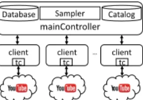
Fig. 1: The experimentation framework
on its assigned probability. From the chosen cell, a random sample, representing the network QoS instance, is selected to be enforced on tc1. During our experiments we also verified
that the clients had a large bandwidth and low delay towards the YouTube cloud such that the network degradation was mainly caused by tc. Note here that by using a trace based sampling approach, we can build a QoS-QoE dataset that is closer to reality than the one based on uniform space sampling. B. Video catalog
Today’s video content providers have huge catalogs of videos that vary in content type. To build QoE prediction models for such providers, we take into consideration this diversity of contents by considering a large number of different videos in our experiments. We build a large catalog of videos of around 1 million different videos supporting HD resolutions (720p and above). This catalog is built by searching the YouTube website using the YouTube Data API with around 4k keywords from Google top trends website for the period of January 2015 to November 2017. We sample this catalog to select a unique video to playout at each experiment. C. The overall experimental framework
Our overall framework consists of a mainController with several clients as shown in Figure 1. The mainController stores the video catalog and provides the network configurations (using the trace based sampling framework) to the clients which perform the experiments. In each experiment, the client, 1) obtains from the mainController the network QoS instance and the video ID, 2) enforces the network QoS using tc, 3) plays out the selected video in a Google Chrome Browser, 4) obtains the traffic features from the encrypted packet traces and the application QoE metrics from the browser, and 5) reports back the results (QoS-QoE tuple) to the mainController which stores the results in a central database. We implement our methodology in a Grid computing environment where up to 30 clients are used to perform the experiments in parallel. We use the Grid5000 [19] and the R2Lab [20] computing platforms for the clients, while the mainController is hosted on an AWS EC2 instance [21]. Such segregation allows large scale experimentations to be carried out by clients distributed
1We do not consider trace samples which have very large values, we only
consider values that are below a certain limit. These limits are 10 Mbps for downlink/uplink bandwidth, 1000 ms for RTT and its variation and 50% for loss rate. Note that almost all the samples in our traces have values within these limits (93% for downlink bandwidth and 98% for the remaining features). We only consider such samples free from outliers to devise our sampling framework.
144p 240p 360p 480p 720p Resolution 0.0 1.0 2.0 3.0 4.0
Chunk Size (MBytes)
# Samples: 136406 207983 245390 401548 857033
Fig. 2: Variation of the video chunk sizes w.r.t resolution (VP9 codec, 30 fps). Total number of samples: 1848360.
geographically. Furthermore, we consider a large number of videos to account for the diversity of load incurred by YouTube videos on the network caused by the different content they present. Overall, we collect a dataset of around 100k unique video playouts. In the next section we discuss the input features and the output QoE metrics we use for building QoE prediction models from this dataset.
IV. THETRAININGDATASET A. Network features
The network features we use to build our models are collected from the encrypted packet traces in each experi-ment. These include the statistical metrics of the average, the maximum, the standard deviation and the 10th to 90th percentiles (in steps of 10) for the downlink throughput (in bits per second), the uplink and downlink interarrival times (in seconds) and the downlink packet sizes (in bytes). A single video session (a video running in a Chrome browser) can correspond to several flows (towards the CDNs identified by the URLs ending with googlevideo.com) at the network layer. We collect these features for all such flows that carry the traffic for each video playout. We end up having a total of 48 features comprising the Finband feature set. With these features, we
believe that we can get a fine grained view of what happens during the video stream.
Chunk information from encrypted traffic. In addition to the above mentioned features and to further improve the modeling, we propose a method to infer the chunk sizes from encrypted flows of YouTube. In adaptive streaming, the video is delivered to the client in chunks. For YouTube, we observe that the audio and the video chunks are requested using separate HTTP requests. Each video chunk is downloaded with a given resolution/bitrate that may vary according to the network conditions. As videos with higher resolution naturally have higher bitrates and vice versa, the video chunk sizes vary with the resolution. Note that the size of the audio chunks is observed to remain the same across resolutions for the same video playout. The variation of the video chunk size (obtained from clear text HTTP traces extracted in the Chrome browser using the chrome.webRequest API) [22] w.r.t each resolution is shown in Figure 2. The figure shows that indeed the size of the video chunks tends to increase for higher resolutions.
To infer the chunk sizes from encrypted traffic, we develop the following method. We assume that for each video flow a
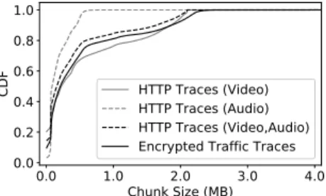
0.0 1.0 2.0 3.0 4.0 Chunk Size (MB) 0.0 0.2 0.4 0.6 0.8 1.0 CDF HTTP Traces (Video) HTTP Traces (Audio) HTTP Traces (Video,Audio) Encrypted Traffic Traces
Fig. 3: CDF of the chunk sizes inferred from the encrypted traces compared to the chunk sizes observed in the clear text HTTP traces (obtained in Google Chrome browser) for the same video sessions
large sized uplink packet corresponds to a chunk request while small packets correspond to acknowledgments in TCP/QUIC based flows. We look at the size of each uplink packet and use K-means clustering to segregate the uplink packet sizes into two clusters; the first cluster represents the acknowledgement packets while the second cluster represents the request packets. Once the uplink request packets are identified, we sum up the amount of data downloaded between the request packets, which represents the chunk sizes. Figure 3 compares the chunks sizes extracted from encrypted traffic traces and the chunk sizes observed in the clear text HTTP traces for the same video sessions. The distribution of the encrypted chunk sizes extracted using our method is close to the combined distribution of audio and video chunks observed in the HTTP traces. Furthermore, the video chunks understandably have larger sizes than audio chunks. As can be noticed, our chunk extraction method cannot distinguish between audio or video chunks, so it does contain some redundant audio chunk in-formation, however, the size of the video chunks especially in view of their large sizes w.r.t audio chunks is still captured. As we will show later in Section V, and thanks to this information on chunk sizes, we will manage to make it considerably helpful in improving the QoE models of YouTube.
Overall, for each video session we obtain an array of chunk sizes extracted from the encrypted traces. We build a feature set composed of the average, the minimum, the maximum, the standard deviation, the 25th, the 50th and the 75th percentiles of the chunk sizes array. This results in the Fchunksfeature set
composed of 7 statistical features. We believe that the upper quartiles in this feature set should capture the information of the video chunks due to their larger size.
In addition to the above mentioned feature sets, we also consider modeling with the five features that are configured on tc. We call these features Foutband as they are not gathered
from traffic traces but rather configured out-of-band on tc. They represent the performance of the underlying network access over which the video is played out.
B. The subjective MOS
The subjective QoE model we use to define our MOS relies on using the ITU recommendation P.1203 [7]. It describes a set of objective parametric quality assessment modules.
These are the audio quality estimation module (Pa), the video quality estimation module (Pv), and the quality integration module (Pq). The Pq module is further composed of the A/V integration (Pav) and buffering impact modules (Pb). The Pv module predicts mean opinion scores (MOS) on a 5-point ACR scale [23]. The Recommendation further describes four different quality modules, one for each mode of ITU-T P.1203, i.e., modes 0, 1, 2 and 3. Each mode of operation has different input requirements ranging from only meta data to frame level information of the video stream. Since our goal in this paper is to target encrypted video streams from a network point of view, we use mode 0 of the model that requires only meta data for each video stream. We consider the video quality only; the audio quality is not considered in this work. The meta data needed to obtain the MOS includes the bitrate, the codec, the duration, the frame rate and the resolution of each chunk. It also considers stalling as well, where for each stall, the media time of stall and its duration are taken as input. The model also considers the ”memory” effect where each stalling duration is assigned a weight depending on its location within the video session. Finally the model considers the device type (mobile/PC), the display size and the viewing distance. In our work we set the device type to be PC, with display size set to 1280x780 and viewing distance to be 250 cm.
Using the meta data for each stream, the outputs of the model include 1) the final audiovisual coding quality score (O.35), 2) the perceptual stalling indication (O.23), and 3) the final media session quality score (O.46). These scores are calculated by the Pv and the Pb modules. O.35 considers the visual quality that is dependent on the resolution and bitrate of playout while O.23 considers stalling and startup delay. Overall the final output of the model is O.46 that considers both O.23 and O.35. We use O.46 as the final MOS and calculate it using a python implementation provided in [24], [25]. This python module requires input meta data of the bitrate, the resolution of each chunk, and the stalling information, if any, for the video played out. We obtain this information from the clear text HTTP traces in the Chrome browser and the YouTube API. Specifically, we extract itag, range, mime and clen parameters for each chunk request to infer the resolution, the codec and the bitrate of each chunk (assuming equal duration of chunks) while the timestamp and the duration of each stalling event is obtained from the YouTube API.
It should be noted here that YouTube videos can play out in either H.264 (mp4) or VP9 (webm) codec while the current version of the ITU-T model is standardized for H.264 codec only; standardization for VP9 is in progress [26]. To get MOS values for VP9, we use the mapping function provided by the authors in [24] to translate the H.264 MOS to a VP9 MOS for videos that play with the VP9 codec.
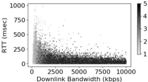
The visualization of the collected dataset is given in Figure 4 that shows the variation of the two network features of downlink bandwidth and RTT with the corresponding MOS. An obvious relationship between QoS and MOS is visible here: as the bandwidth increases (or RTT decreases), the
Fig. 4: Variation of the ITU MOS w.r.t configured bandwidth and RTT. # samples: 104504. Unique video count: 94167.
0 2000 4000 6000 8000 10000 Bandwidth (kbps) 0.0 0.2 0.4 0.6 0.8 1.0 CDF DL_BW UL_BW (a) Bandwidth 0 200 400 600 800 1000 RTT and its variation (msec) 0.0 0.2 0.4 0.6 0.8 1.0 CDF RTT std_RTT
(b) RTT and its variation Fig. 5: The CDF for Foutbandenforced on tc
MOS increases. Notice the absence of experiments in regions where the bandwidth and the RTT both are high. This non-uniformity comes from our trace based sampling framework (Section III-C) where TCP based measurements achieve high throughput with low RTT and vice versa.
C. Statistical analysis of the collected dataset
In this section, we present the statistical analysis of our dataset to get insights into the variation of the network QoS, the observed application QoS metrics (startup delay, stalls, quality switches and resolution of playout) and the MOS.
1) Network Features: Figure 5 shows the distribution of the network features configured on tc (Foutband) using our
sam-pling methodology. From these figures, we can see that 80% of the experiments have the uplink bandwidth less than 1.7 Mbps while the downlink bandwidth remains below 5 Mbps. Similarly, the RTT and its variation are mostly concentrated around 100 ms while loss rate is less than 2.3% for 90% of the total experiments (CDF for loss rate not shown here).
In Finband, the average downlink throughput per playout
gets a mean value of 1.89 Mbps compared to the mean of the configured downlink bandwidth of 2.72 Mbps (average of DL BW in Figure 5a). Furthermore, the mean values for the average downlink and uplink packet interarrival times are 13 and 14 msecs respectively while the downlink average packet size gets a mean value of 1485 bytes.
In Figure 6, we show the CDF of the statistical features of the chunk sizes (Fchunks). Note that the minimum chunk size
can be very small; for 80% of our experiments, we observe a chunk size less than 8.9 KB. On the other hand, the maximum chunk size can go up to 2.19 MB. The average and the standard deviation of the chunk size have similar distributions with median values of 400 KB and 493 KB respectively.
0 1 2 3 4 5 Chunk size (MB) 0.2 0.4 0.6 0.8 1.0 CDF AVG STD MIN MAX
Fig. 6: The CDF of the statistical chunk size features (Fchunks)
0 10 20 30 Startup delay (sec) 0.0 0.2 0.4 0.6 0.8 1.0 CDF
Our work (100k playouts) Prior work (300M views)
(a) Startup delay
0 10 20 30 40 50 Number of stalling events 0.4
0.6 0.8 1.0
CDF
(b) Number of stalling events
0 10 20 30 Total stalling duration (sec) 0.0 0.2 0.4 0.6 0.8 1.0 CDF
(c) Total stalling duration
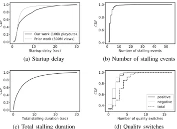
0 5 10 15 Number of quality switches 0.4 0.6 0.8 1.0 CDF positive negative total (d) Quality switches Fig. 7: The CDF of the startup delay, the stallings and the quality switches
2) Startup delay: In our work, we define a timeout for each experiment to be 30 seconds. We consider this threshold value based on the findings of prior subjective studies on user engagement with a large number of real users. For example, authors in [27] study a dataset of 23 million views and show that the video abandonment rate went up to 80% for videos with startup delay higher than 30 seconds. In another study based on a dataset of 300 million video views, around 98% of the total views had a startup delay of less than 30 seconds [28]. In our dataset, 93% videos start to play within 30 seconds while the remaining 7% timeout. The variation of the startup delays for the videos that started playing is shown in Figure 7a where the distribution is observed to be non uniform with 80% of experiments having a startup delay of less than 10 seconds. As seen in Figure 7a, this observation has also been made in prior work [28] based on real user measurements, with an even more pronounced skewness towards lower startup delays.
3) Stalls: Since YouTube uses ABR, we expect that stalls or rebufferings should be rare events. Indeed we observe the same in our dataset as only 12% of the video playouts suffer from stalling. We plot the CDF of the number of stalling events and the total stalling duration per playout in Figures 7b and 7c considering videos that at least had one stall. From the figure, we can see that around 40% of the videos that stalled had only one stall while 70% of the total stalled videos suffered up to two stalls only. Overall, 80% of the stalled videos had the total stalling duration less than 7 seconds (Figure 7c).
1 2 3 4 5 Average resolution score 0.0 0.2 0.4 0.6 0.8 1.0 CDF
(a) Average resolution score
1 2 3 4 5 MOS 0.0 0.2 0.4 0.6 0.8 1.0 CDF QoE_ITU_023 QoE_ITU_035 QoE_ITU_046 (b) ITU-T MOS
Fig. 8: The CDF of the average resolution score, r and MOS
4) Quality switches: Contrary to stalls, we observe that quality switches are more common in our dataset due to ABR; 73% of the video playouts have at least one quality switching event. A quality switch can either be ”positive” i.e. the resolution of playout increases from low resolution to high, or it can be ”negative” if the resolution decreases. The CDF of these events is shown in Figure 7d where both the positive and the negative switch events are shown to have similar distributions.
5) The average resolution score: We measure the resolution of each chunk from the HTTP traces and assign a score to the resolution of each chunk, i.e., 1 for 144p, 2 for 240p, 3 for 360p, 4 for 480p and 5 for 720p and above. The average resolution score, r, corresponds to the mean of these scores and ranges from 1 to 5. Figure 8a shows that the distribution r is biased towards higher values. This is due to the measurement datasets used in our sampling methodology (Section III-A) which result in more experiments with good network conditions as seems to be the case with real users.
In our dataset, we observe that the highest resolution mostly goes up to 720p even though we used videos that propose even higher resolution (upto 1080p). Since the viewport in the Chrome browser in our experiments had size of 1280x780, the YouTube player seems not requesting higher resolution segments. This suggests that YouTube client considers the viewport in choosing the quality of playout.
6) The ITU P.1203 MOS: Finally, the CDF of the resulting ITU MOS is shown in Figure 8b. The maximum values for O.23 are between 4.5 and 5.0 which is also true for the MOS (O.46). However, the CDF for O.46 is more similar to O.35 which means that in our dataset, the ITU MOS is affected more by the resolution and bitrate of playout compared to the rebufferings (startup delay and stalls).
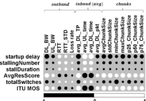
D. Correlation analysis between network QoS and QoE To understand the relationship between the input network features and the QoE, we measure the corresponding Pearson correlation coefficients and plot the correlation matrix of the feature sets in Figure 9. From the figure, we can see that the startup delay, the average resolution score and the MOS have strong correlation with all the features of Foutbandexcept
for the packet loss rate while the stall duration, the stalling number (total number of stalls in a given playout) and the quality switches show little correlation with Foutband. For the
Fig. 9: Correlogram for network QoS, app QoS and MOS
arrival times show the strongest correlation with the QoE metrics (except for stalls and number of switches) while the downlink packet size shows a comparatively lower correlation. Finally, for Fchunks, the correlation with the QoE metrics
is again strong except for the metrics related to stalls. The number of switches shows a better correlation here compared to the preceding two features sets with minimum chunk size showing the strongest correlation. To summarize, all the QoE related metrics have good correlation with our network feature sets except for stalling; we will discuss the potential reason for this in the next section where we evaluate the ML models built from these features.
V. EVALUATION OF THEML MODELS
In this section, we discuss the performance of the ML mod-els built using our dataset. We try to predict application QoS metrics and MOS using network QoS. We aim at assessing how well the following questions can be answered:
1) Predict if the video starts to play or not. 2) If the video starts, estimate the startup delay. 3) Predict if the video plays out smoothly or has stalls. 4) Predict if there are any quality switches.
5) Estimate the average resolution of playout. 6) Estimate the final QoE in terms of the ITU MOS. We consider three sets of features; Foutband, Finband and
Finband+chunk to build predictive ML models. Our work
considers both the classification and the regression scenarios as we have both discrete as well as continuous output labels. A. Estimating startup delay
To estimate the startup delay, we need to first classify if the video started to play out. We classify the video as started if the startup delay is less than 30 seconds and not started if a timeout occurs. Considering this binary classification problem, we train a Random Forest (RF) ML model (using python Scikit-Learn library [29] in default parameter configurations) with our dataset and evaluate its accuracy using k-fold cross validation. In k-fold cross validation, the dataset is split into training and validation sets k times randomly. The model is then trained with the training set and tested with the validation set k times to get k accuracy scores. The final accuracy score is then the average of these k scores. The metric for classification
Feature Set Class Count Prec Recall F1 Avg F1
Foutband 01 1045187401 85.498.9 84.599.0 85.098.9 92.0
Finband 01 1045187401 95.499.7 95.199.7 95.299.7 97.4
Finband+chunks 01 1045187401 100.099.8 100.099.9 100.099.9 99.9
TABLE I: ML classification accuracy of predicting video start up. Class 0: not started (startup delay > 30 seconds). Class 1: video started to play.
Feature Set Regression Algo RMSE Foutband Linear RegressionRF Regression 4.312.97
Finband Linear RegressionRF Regression 2.992.85
Finband+chunks Linear RegressionRF Regression 2.982.66
TABLE II: RMSE (in seconds) for the predicted startup delay
accuracy we use is the F1-Score2 with k = 3 and a data split ratio of 80:20 for training and validation. The ML performance resulting from training RF with each of the three feature sets is given in Table I. The models obtain over 90% accuracy for the three sets. Furthermore, the performance improves if Finbandis used compared to Foutband. With Finband+chunks,
we get the best average F1-score of over 99%.
We now try to estimate the startup delay using ML regres-sion models trained with started videos. We compare models based on Linear Regression and Random Forest (RF) Regres-sion. The evaluation is done based on the well known metric of Root Mean Squared Error (RMSE) given by
q
E[ ˆ(y − y)2],
where y are the true labels and ˆy are the predictions made by the regression model. The results are shown in Table II where we obtain the minimum RMSE of 2.66 seconds using Random Forest (RF) Regression with Finband+chunks. A noticeable
observation is that we can obtain a reasonably low RMSE of 2.97 seconds if we use RF Regression with Foutband,
which can be explained by the fact that the startup delay is determined by the initial buffering time, which in turn is determined by network performance. This can justify in practice the use of out-of-band measurements alone to predict startup delay without relying on accessing the video traffic i.e. predict startup delay without playing out the videos.
B. Predicting quality switches and stalls
In this section, we present the results of the ML models for detecting the quality switches and the stallings. As YouTube uses ABR, the resolution of the video played out can change depending upon the network conditions. To detect these quality changes, we consider a binary classification scenario where the output label 0 corresponds to a video being played out with constant quality, while the label is 1 if the video changes its quality at least once. Using the same methodology of
2The F1-score is a measure to gauge the accuracy of the ML model by
taking into account both the precision and recall. It is given by 2pr/(p + r), where p and r are the precision and recall of the ML model respectively.
Feature Set Class Count Prec Recall F1 Avg F1 Foutband 01 2857775941 44.578.4 40.681.0 42.579.7 61.1
Finband 01 2857775941 55.482.8 54.183.6 54.783.2 68.9
Finband+chunks 01 2857775941 87.994.1 84.295.6 86.094.9 90.4
TABLE III: ML classification accuracy of detecting quality (resolution) switches. Class 0: video plays at constant quality. Class 1: there are quality switches.
Feature Set Class Count Prec Recall F1 Avg F1
Foutband 01 9180412714 89.551.0 97.816.6 93.425.0 59.2
Finband 01 9180412714 89.754.8 97.918.7 93.627.9 60.8
Finband+chunks 01 9180412714 90.259.8 98.022.1 93.932.2 63.1
TABLE IV: ML classification accuracy of detecting stalls. Class 0: video plays smoothly. Class 1: video has stalls.
Section V-A, we obtain the performance results given in Table III. We observe that with feature sets Foutband and
Finband we do not get good accuracy scores suggesting that
the conventional network and traffic features used in prior works are not sufficient to predict quality switches from encrypted traces. However, if we include the Fchunks feature
set for prediction, we can see a significant improvement with over 90% precision and recall for quality switch detection. This improvement comes from the relationship between chunk sizes and the corresponding resolutions (Figure 2).
For the scenario of detecting stalls we again consider a binary classification scenario where the label 0 corresponds to video playing out smoothly without any stall while a label of 1 is assigned if there is stalling in the playout. The accuracy of the obtained ML model is shown in Table IV. A surprising observation here is that the model suffers from low recall for stall detection suggesting that the model fails to detect stalls. This is contrary to what is seen in the literature where similar statistical features were used. The reason is that prior works for stall detection used datasets mostly consisting of videos without ABR; in [10] the videos played out with constant quality, while in [4], the dataset had 97% videos that did not use ABR. However in our work, we use ABR for all the experiments and use a very diverse set of video contents, which explains why the statistical network features fail to detect stalls. Indeed, the features we consider capture the network QoS holistically without considering the temporal aspects of playout. As we know that stalling can occur at any time instant during playout, capturing those temporal degradations is very important in order to accurately detect stalls. For example, the video bitrate at the time of stall might be suddenly high while being low otherwise. In such a scenario, the overall statistical features would look similar to a normal playout making stall detection difficult. We believe that in the presence of ABR, stalls become rare events that depend on the temporal properties of the video, and thus, can hardly be detected
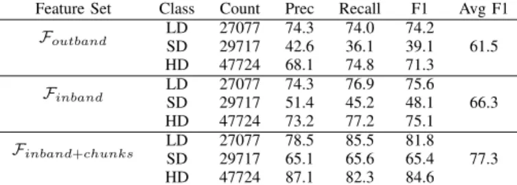
Feature Set Class Count Prec Recall F1 Avg F1
Foutband LDSD 2707729717 74.342.6 74.036.1 74.239.1 61.5 HD 47724 68.1 74.8 71.3 Finband LDSD 2707729717 74.351.4 76.945.2 75.648.1 66.3 HD 47724 73.2 77.2 75.1 Finband+chunks LDSD 2707729717 78.565.1 85.565.6 81.865.4 77.3 HD 47724 87.1 82.3 84.6
TABLE V: ML classification accuracy of detecting resolution Feature Set Regression Algo RMSE
Foutband Linear RegressionRF Regression 0.6840.470
Finband Linear RegressionRF Regression 0.4540.428
Finband+chunks Linear RegressionRF Regression 0.4230.333
TABLE VI: RMSE of the predicted MOS
without features capturing the video content itself, in particular its burstiness. We leave the exploration of this idea for a future research with focus on video content and its characterization. C. Estimating average resolution of playout
To build a ML model that detects the average resolution of playout, we convert the average resolution score, r (defined in Section IV-C5) into three resolution levels: 1) low definition (LD), if 1 ≤ r ≤ 3.5, 2) standard definition (SD), if 3.5 < r ≤ 4.5, and 3) high definition (HD), if 4.5 < r ≤ 5.
For a classification scenario with three output labels, the model performance using Random Forests (RF) is given in Table V. We again see that by using Fchunks, we improve
the overall F1-scores of the model because of the positive relationship between chunk size and resolution. However, the individual F1-scores for SD are lower compared to LD and HD. This is because SD is an intermediary class and usually the accuracy for such classes is lower compared to edge classes in cases such as ours where the output labels and input features form a monotonic relationship. Overall, the best performance is obtained for class HD where a precision of 87% is achieved.
D. Estimating the ITU MOS
We consider both regression and classification scenarios for predicting the MOS based on the ITU P.1203 model. Table VI shows the RMSE with the RF and the linear regression models. Similar to the observation in Section V-A, the RMSE decreases with enrichment of the input set with relevant features. The lowest RMSE of 0.33 is obtained using the Finband+chunks
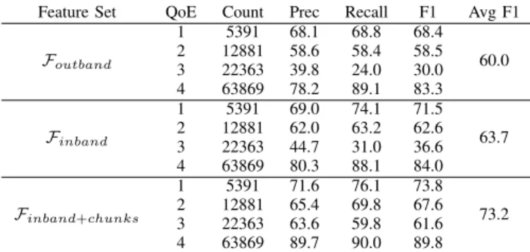
feature set and RF regression. Table VII shows the MOS prediction results where we quantize the MOS into 4 classes and then train the RF classifier. As we enrich the feature sets, we see improvement in performance across all classes. With Finband+chunks, the precision per class ranges from
63% to 90% while the recall per class ranges from 60% to 90%. Overall, we get an average F1-score of 73%. Note that the accuracy for the intermediary classes 2 and 3 is lower
Feature Set QoE Count Prec Recall F1 Avg F1 Foutband 1 5391 68.1 68.8 68.4 60.0 2 12881 58.6 58.4 58.5 3 22363 39.8 24.0 30.0 4 63869 78.2 89.1 83.3 Finband 1 5391 69.0 74.1 71.5 63.7 2 12881 62.0 63.2 62.6 3 22363 44.7 31.0 36.6 4 63869 80.3 88.1 84.0 Finband+chunks 1 5391 71.6 76.1 73.8 73.2 2 12881 65.4 69.8 67.6 3 22363 63.6 59.8 61.6 4 63869 89.7 90.0 89.8
TABLE VII: ML classification accuracy with quantized MOS. Bins: 1) 1.0 – 2.0, 2) 2.0 – 3.0, 3) 3.0 – 4.0, 4) 4.0 – 5.0). Predicted Class 1 2 3 4 Original 1 0.76 0.22 0.01 0.00 2 0.11 0.71 0.15 0.03 3 0.01 0.13 0.59 0.27 4 0.00 0.01 0.08 0.90
TABLE VIII: MOS confusion matrix using Finband+chunks
compared to the edge classes 1 and 4 due to the monotonic relationship between our features and the MOS. Furthermore, if we look at the confusion matrix in Table VIII, we can observe that the misclassifications mostly occur to the adjacent classes.
VI. LIMITATIONS
The dataset presented in this work was collected using Google Chrome browser based on Linux machines; we do not consider mobile devices or other browsers. The effect of network QoS on QoE may vary across different platforms and devices which is not handled by the models in this work.
Our dataset is based on TCP based video flows for YouTube collected in April 2018. Over time, we expect that video content providers can change their video delivery mechanisms which would limit the applicability of our model to be used in future. So, over a period of time, the training data would have to be re-collected again to ensure that the models are updated according to the latest version of the targeted video provider. The results for the MOS prediction are based on only one set of parameters used for the ITU P.1203 model. With a different set of parameters e.g. a different screen size, the resulting MOS distribution will also change which would change the performance of the ML models as well.
VII. CONCLUSION
In this paper we presented our methodology for building QoS-QoE prediction models from encrypted Internet video traffic using controlled experimentation and machine learning. The models presented predict not only the application level QoS features but also the subjective QoE modeled as MOS according to ITU-T P.1203. Overall our experimentation ap-proach is re-usable to construct large datasets in distributed computing environments for any video content provider. The future work will focus on developing methods to improve the
low stall detection accuracy of our models by considering met-rics reflecting the content of videos itself, and will elaborate further on the capacity of ABR to adapt to fast changes in video content under different network conditions.
REFERENCES
[1] “Cisco Visual Networking Index (VNI) Forecast,” 2016, https://www.cisco.com/c/en/us/solutions/service-provider/visual-networking-index-vni/index.html.
[2] “Ericsson Mobility Report, June 2018,” 2018,
https://www.ericsson.com/assets/local/mobility-report/documents/2018/ ericsson-mobility-report-june-2018.pdf.
[3] T. Hoßfeld, M. Seufert, M. Hirth, T. Zinner, P. Tran-Gia, and R. Schatz, “Quantification of youtube qoe via crowdsourcing,” in Multimedia (ISM), 2011 IEEE International Symposium on, Dec 2011, pp. 494–499. [4] G. Dimopoulos, I. Leontiadis, P. Barlet-Ros, and K. Papagiannaki, “Measuring video qoe from encrypted traffic,” in Proceedings of the 2016 Internet Measurement Conference, 2016, pp. 513–526.
[5] R. K. P. Mok, E. W. W. Chan, and R. K. C. Chang, “Measuring the quality of experience of http video streaming,” in 12th IFIP/IEEE Int’l Symp. on Integrated Network Management, May 2011, pp. 485–492. [6] M. H. Mazhar and Z. Shafiq, “Real-time video quality of experience
monitoring for https and quic,” in IEEE INFOCOM 2018 - IEEE Conference on Computer Communications, April 2018.
[7] ITU, “Parametric bitstream-based quality assessment of progressive download and adaptive audiovisual streaming services over reliable transport,” ITU-T Rec. P.1203, 2017.
[8] “Code and Datasets,” 2018, https://github.com/mjawadak/youtubeapi. [9] I. Orsolic, D. Pevec, M. Suznjevic, and L. Skorin-Kapov, “A machine
learning approach to classifying youtube qoe based on encrypted net-work traffic,” Multimedia Tools and Applications, vol. 76, 2017. [10] V. Aggarwal, E. Halepovic, J. Pang, S. Venkataraman, and H. Yan,
“Prometheus: Toward quality-of-experience estimation for mobile apps from passive network measurements,” in HotMobile ’14. ACM, 2014. [11] D. Joumblatt, J. Chandrashekar, B. Kveton, N. Taft, and R. Teixeira, “Predicting user dissatisfaction with internet application performance at end-hosts,” in 2013 Proceedings IEEE INFOCOM, April 2013. [12] K. T. Chen, C. C. Tu, and W. C. Xiao, “Oneclick: A framework for
measuring network quality of experience,” in IEEE INFOCOM, 2009. [13] M. Seufert, N. Wehner, F. Wamser, P. Casas, A. D’Alconzo, and P.
Tran-Gia, “Unsupervised qoe field study for mobile youtube video streaming with yomoapp,” in QoMEX, May 2017, pp. 1–6.
[14] M. Katsarakis, R. C. Teixeira, M. Papadopouli, and V. Christophides, “Towards a causal analysis of video qoe from network and application qos,” in Proceedings of the Internet QoE’16. ACM, 2016.
[15] “Linux Traffic Control,” 2018, http://lartc.org/.
[16] M. J. Khokhar, N. A. Saber, T. Spetebroot, and C. Barakat, “On active sampling of controlled experiments for qoe modeling,” in Proceedings of the Internet QoE’17. ACM, 2017.
[17] “RTR-Netz open dataset,” 2017, https://www.netztest.at/en/Opendata. [18] “MobiPerf,” 2018, https://www.measurementlab.net/tests/mobiperf/. [19] “Grid5000,” 2018, https://www.grid5000.fr.
[20] “R2Lab,” 2017, https://r2lab.inria.fr/index.md. [21] “AWS EC2,” 2018, https://aws.amazon.com/ec2/.
[22] “WebRequest,” 2018, https://developer.chrome.com/extensions/webRequest. [23] ITU-T, “Subjective video quality assessment methods for multimedia
applications,” ITU-T Recommendation P.910, 2008.
[24] W. Robitza et al., “HTTP Adaptive Streaming QoE Estimation with ITU-T Rec. P.1203 Open Databases and Software,” in 9th ACM Multimedia Systems Conference, Amsterdam, 2018.
[25] “ITU P.1203 Python implementation,” 2018, https://github.com/itu-p1203/itu-p1203.
[26] “Ericsson QoE report,” 2017, https://www.ericsson.com/en/ericsson- technology-review/archive/2017/video-qoe-leveraging-standards-to-meet-rising-user-expectations.
[27] S. S. Krishnan and R. K. Sitaraman, “Video stream quality impacts viewer behavior: Inferring causality using quasi-experimental designs,” in IMC ’12. ACM, 2012, pp. 211–224.
[28] F. Dobrian, V. Sekar, A. Awan, I. Stoica, D. Joseph, A. Ganjam, J. Zhan, and H. Zhang, “Understanding the impact of video quality on user engagement,” SIGCOMM CCR, vol. 41, no. 4, Aug. 2011.