HAL Id: hal-01661263
https://hal.archives-ouvertes.fr/hal-01661263
Preprint submitted on 11 Dec 2017
HAL is a multi-disciplinary open access
archive for the deposit and dissemination of sci-entific research documents, whether they are pub-lished or not. The documents may come from teaching and research institutions in France or abroad, or from public or private research centers.
L’archive ouverte pluridisciplinaire HAL, est destinée au dépôt et à la diffusion de documents scientifiques de niveau recherche, publiés ou non, émanant des établissements d’enseignement et de recherche français ou étrangers, des laboratoires publics ou privés.
José de Sousa, Anne-Célia Disdier, Carl Gaigné
To cite this version:
Export Decision under Risk
José DE SOUSA, Anne-Célia DISDIER, Carl GAIGNÉ
Working Paper SMART – LERECO N°17-10
December 2017
UMR INRA-Agrocampus Ouest SMART - LERECO
Les Working Papers SMART-LERECO ont pour vocation de diffuser les recherches conduites au sein des unités SMART et LERECO dans une forme préliminaire permettant la discussion et avant publication définitive. Selon les cas, il s'agit de travaux qui ont été acceptés ou ont déjà fait l'objet d'une présentation lors d'une conférence scientifique nationale ou internationale, qui ont été soumis pour publication dans une revue académique à comité de lecture, ou encore qui constituent un chapitre d'ouvrage académique. Bien que non revus par les pairs, chaque working paper a fait l'objet d'une relecture interne par un des scientifiques de SMART ou du LERECO et par l'un des deux éditeurs de la série. Les Working Papers SMART-LERECO n'engagent cependant que leurs auteurs.
The SMART-LERECO Working Papers are meant to promote discussion by disseminating the research of the SMART and LERECO members in a preliminary form and before their final publication. They may be papers which have been accepted or already presented in a national or international scientific conference, articles which have been submitted to a peer-reviewed academic journal, or chapters of an academic book. While not peer-reviewed, each of them has been read over by one of the scientists of SMART or LERECO and by one of the two editors of the series. However, the views expressed in the SMART-LERECO Working Papers are solely those of their authors.
Export Decision under Risk
José DESOUSA
Université Paris-Sud, RITM and Sciences-Po Paris, LIEPP, France
Anne-Célia DISDIER
Paris School of Economics-INRA, France
Carl GAIGNÉ
INRA, UMR1302 SMART-LERECO, Rennes, France Université Laval, CREATE, Québec, Canada
Acknowledgments
We thank Treb Allen, Manuel Amador, Roc Armenter, Nick Bloom, Holger Breinlich, Lorenzo Caliendo, Maggie Chen, Jonathan Eaton, Stefania Garetto, Stefanie Haller, James Harrigan, Keith Head, Oleg Itskhoki, Nuno Limão, Eduardo Morales, Peter Morrow, Gianmarco Otta-viano, John McLaren, Marc Melitz, John Morrow, Denis Novy, Mathieu Parenti, Thomas Philip-pon, Ariell Reshef, Veronica Rappoport, Andrés Rodríguez-Clare, Claudia Steinwender, Daniel Sturm, Alan Taylor, and seminar and conference participants at CEPII, DEGIT (U. of Geneva), EIIT (U. of Michigan), George Washington U., Harvard Kennedy School, EIIE, LSE, ETSG, U.C. Berkeley, U.C. Davis, U. of Caen, U. of Strathclyde, U. of Tours, U. of Virginia, and SED for their helpful comments. This work is supported by the French National Research Agency through the Investissements d’Avenir program, ANR-10-LABX-93-01, and by the CEPREMAP.
Corresponding author
Carl Gaigné
INRA, UMR1302 SMART-LERECO 4, allée Adolphe Bobierre
CS 61103
35011 Rennes, France
Email: [email protected]
Téléphone / Phone: +33 (0)2 23 48 56 08 Fax: +33 (0)2 23 48 53 80
Les Working Papers SMART-LERECO n’engagent que leurs auteurs.
Export Decision under Risk
Abstract
Using firm and industry data, we unveil two empirical regularities: (i) Demand uncertainty not only reduces export probabilities but also decreases export quantities and increases export prices; (ii) The most productive exporters are more affected by higher industry-wide expenditure volatility than are the least productive exporters. We rationalize these regularities by developing a new firm-based trade model wherein managers are risk averse. Higher volatility induces the reallocation of export shares from the most to the least productive incumbents. Greater skewness of the demand distribution and/or higher trade costs weaken this effect. Our results hold for a large class of consumer utility functions.
Keywords: firm exports, demand uncertainty, risk aversion, expenditure volatility, skewness
Décision d’exportation en environnement risqué
Résumé
En utilisant les données d’entreprise et d’industrie, nous mettons e évidence deux régularités empiriques : (i) L’incertitude de la demande étrangère réduit les ventes à l’exportation, la prob-abilité d’exporter, et l’efficacité des politiques commerciales; (ii) Les grandes entreprises sont les exportateurs les plus affectés par l’incertitude. Nous rationalisons ces régularités à l’aide d’un nouveau modèle de commerce international dans lequel les entreprises agissent dans un environnement incertain. On montre qu’une plus grande incertitude induit une réallocation des parts de marché des entreprises productives vers les moins productives. Cependant, des bar-rières aux échanges élevés réduit ce phénomène de réallocation. Nos résultats tiennent pour une large classe de fonctions d’utilité.
Mots-clés: exportations de firmes, incertitude de la demande, aversion au risque aversion, poli-tique commerciale
Export Decision under Risk
1. Introduction
We study the impact of demand uncertainty on firm export decisions.1 Most trade theory
as-sumes that demand in foreign markets is known with certainty. Accordingly, firms know their exact demand functions, and only market size plays a key role in export performance. However, recent surveys of leading companies note that market/demand uncertainty is their top business
driver.2 This view is consistent with empirical evidence of the impact of demand uncertainty
on a wide variety of economic outcomes, such as investment, production, and pricing decisions (seeBloom,2014).
Despite a growing and recent literature on the impact of uncertainty on trade, little is known about how firms respond to demand uncertainty in foreign markets. In this paper, we study the impact of demand uncertainty in foreign markets on firms’ export quantities and prices (intensive margin) and export entry/exit decisions (extensive margin).
Our theory is motivated by reduced-form evidence of the effect of foreign expenditure uncer-tainty on French manufacturing exports. We observe the destination countries to which firms export and the products they sell over the 2000-2009 period. We match these firm-level export data with industry-wide measures of expenditure uncertainty in the destination countries, as
proxied by the observed central moments of absorption:3 the expected value, the variance (or
volatility), and the skewness.
We unveil two empirical regularities regarding the role of industry-wide expenditure uncertainty in the intensive and extensive margins of firm exports. First, firm export decisions in a destina-tion market are significantly affected by the central moments of the expenditure distribudestina-tion of that destination. The expected values of expenditure (the first moment) and skewness (the third moment) positively affect both the probability of entry and the export quantities while reducing the prices and the probability of exit. By contrast, the volatility – or variance – of expenditure (the second moment) produces the opposite effects, reducing both the probability of entry and the export quantities while increasing prices and the probability of exit.
Second, the responses of exporting firms to industry-wide expenditure uncertainty are hetero-geneous. As firms differ in size and productivity, they might be differently affected by un-certainty. Our estimations reveal that an increase in expenditure volatility reduces the differ-1Due to the practical difficulties of separating risky events from uncertain events, we followBloom(2014) in referring to a single concept of uncertainty, which captures a mixture of risk and uncertainty. The terms ‘risk’ and ‘uncertainty’ are thus used interchangeably.
2See, for instance, the Capgemini surveys of leading companies that can be publicly accessed for2011,2012, and2013.
ence in export sales between high- and low-productivity firms. More precisely, for a given industry-destination-year triplet, the decrease in export sales due to volatility is greater for high-productivity firms than for low-productivity ones. We also highlight that, for a given industry-year pair, the more productive firms favor destination countries with low volatility and high skewness.
Interestingly, this first empirical regularity shows that uncertainty affects not only the export entry/exit decisions but also the quantities exported and prices. Explaining the effects of un-certainty on both the intensive and the extensive margins of trade is theoretically challenging. Real option effects may explain the extensive margin result. Given the sunk costs of accessing foreign markets, uncertainty makes firms more cautious about serving a new market and de-lays the entry of exporters into new markets. However, having entered, reducing or increasing quantities and prices does not lead to the loss of an option value (from waiting to enter). The intensive margin is an easily reversible action. By assuming risk-averse managers, we develop a new theory allowing us to rationalize these empirical regularities.
The model features three key ingredients: (i) managers are averse to both risk and downside losses, (ii) firms face the same industry-wide uncertainty over expenditures, and (iii) managers make decisions about entry/exit and production/prices before expenditure uncertainty is re-vealed. Firms produce under monopolistic competition and are heterogeneous in productivity, which affects the decision of whether to enter an export market. Having entered, exporters choose strategic variables (price or quantity) before the output reaches the market. Therefore, foreign expenditures or market prices can change between the time quantities are set and the time of delivery due to random shocks, such as changes in consumer preferences, income, cli-matic conditions, opinion leaders’ attitudes, or competing products’ popularity.
One question is why are firm managers risk averse? Managers and shareholders of exporting firms might be risk averse because if uncertainty is common to all firms, risk is non-diversifiable (Grossman and Hart, 1981). However, there are various reasons why the manager of an ex-porting firm might be risk averse even if shareholders are risk neutral: (i) bankruptcy costs
might be high (Greenwald and Stiglitz,1993), (ii) exchange rate risk is not adequately hedged
(Wei,1999), (iii) open-account terms are common in trade finance and allow importers to delay
payment for a certain time following the receipt of goods (Antràs and Foley, 2015), and (iv)
managers’ human and financial capital (through their equity shares) are disproportionately tied
up in the firms they manage (Bloom, 2014). Thus, in making all of their economic decisions,
managers take into account their risk exposure (Panousi and Papanikolaou(2012)).
To capture managers’ willingness to pay a risk premium to avoid uncertainty, we draw on ex-pected utility theory and conduct a mean-variance-skewness analysis. Risk-averse behavior is
the literature on production decisions under risk and imperfect competition, an increase in risk (as measured by higher variance of the random variable) raises the risk premium and decreases
output when the decision maker is risk averse (Klemperer and Meyer,1986). Nevertheless, the
variance does not distinguish between upside and downside risk, while managers can be more
sensitive to downside losses than to upside gains (Menezes et al.,1980). Skewness can provide
information about the asymmetry of the expenditure distribution and, thus, about downside risk exposure. For a given mean and variance, countries with more right-skewed expenditure distri-butions provide better downside protection or less downside risk.
Our model leads to theoretical predictions that rationalize our reduced-form estimations. As expected, the probability of exporting decreases with expenditure volatility but increases with its mean and skewness. We also show that the equilibrium certainty-equivalent quantities, which incorporate the risk premium, are negatively correlated with the volatility of expenditures but positively affected by its mean and skewness.
Further, even if firms face the same industry-wide expenditure volatility, we show that they do react differently to an increase in volatility. In this case, risk aversion and differences in productivity lead to the reallocation of market shares. An increase in expenditure volatility may impede the entry of some producers into the international market and force others to cease exporting, which in turn, may increase the market shares of incumbent exporting firms. Addi-tionally, changes in volatility modify the relative prices of the varieties supplied, leading to the reallocation of market shares across incumbent exporters.
Hence, the effects of industry-specific volatility uncertainty on the export performance of in-dividual firm are not a priori clear. A key result is that an increase in volatility induces the reallocation of market shares from the most to the least productive exporters. The reason is that greater expenditure volatility makes the most productive exporters the most exposed. As high-productivity firms produce larger quantities, their profits are more sensitive to an increase in expenditure variation. Consequently, they reduce their certainty-equivalent quantities relatively more than low-productivity exporters. The market shares of the least productive exporters may
thus grow.4 However, the reallocation effect is weakened when trade barriers increase or/and
the expenditure distribution becomes more right-skewed.
It is worth stressing that our model matches traditional facts concerning the role of trade costs and firm heterogeneity in the trade literature. The main results hold for a large class of consumer utility functions, and unlike trade models of monopolistic competition without uncertainty, the markup is not constant even if demand is isoelastic. In other words, expenditure uncertainty and risk-averse managers allow for variable markups (even under constant elasticity of substitution 4Note that the least productive exporters are medium-sized firms, as small firms are not productive enough to export.
(CES) preferences).
Related Literature
This paper complements a recent body of the literature on the heterogeneous effects of
macroe-conomic uncertainty on individual firms. First, Bloom et al. (2007) highlight a “cautionary
effect” such that greater uncertainty reduces the responsiveness of firms’ R&D and investments to changes in productivity. The investment behavior of large firms is consistent with a partial irreversibility model in which uncertainty dampens the short-run adjustment of investment to demand shocks. In a different setting, we also capture a cautionary effect or “risk-averseness effect” of expenditure uncertainty on export behavior such that greater uncertainty reduces the responsiveness of firms’ exports to changes in productivity. This effect leads to the reallocation of market shares from the most to the least productive exporters. In this way, we provide a new explanation for declines in aggregate productivity growth following uncertainty shocks. As the reallocation of resources across heterogeneous firms is a key factor in explaining aggregate
pro-ductivity growth (Foster et al.,2008;Melitz and Polanec,2015), higher expenditure uncertainty
can slow productivity growth.
Second, Fillat and Garetto(2015) document that exporters and multinationals, which are
typi-cally large firms, face higher risk exposure that makes their profits more sensitive to the state of the global economy. The reason is that entering a foreign market is a source of risk expo-sure when aggregate demand is subject to fluctuation and entry involves a sunk cost. Following a negative shock, risk-averse large firms are reluctant to exit the foreign market because they would forgo the sunk cost they paid to enter. This higher risk exposure commands a higher return in equilibrium for exporters and multinationals compared to domestic firms. We adopt a different perspective by focusing on the role of uncertainty in extensive and intensive export decisions. We argue that firms face aggregate expenditure uncertainty when the strategic vari-ables are chosen. The larger the firms, the more they produce and the more exposed they are to
ex postprice variation because of expenditure variation.
Our paper is also related to the literature on risk and trade. Expected utility theory was used
to analyze international trade under risk by Turnovsky(1974) and Helpman and Razin(1978)
but with perfect competition. More recently, the trade literature has witnessed renewed interest
in studying uncertainty with imperfect competition (e.g.,Nguyen,2012;Ramondo et al.,2013;
Handley,2014;Lewis,2014;Novy and Taylor,2014;Feng et al.,2016;Héricourt and Nedon-celle,2017;Handley and Limao,ming). Following a line of reasoning similar to ours,Esposito
(2016) andGervais(2016) also assume risk averse managers.Gervais(2016) develops a model
of international trade in homogeneous intermediate inputs with uncertainty in the delivery of
inputs, while Esposito(2016) focuses on demand complementarities across markets under
un-certainty. By contrast, our paper explores the reallocation of export shares across firms within a market under uncertainty. Furthermore, we use a more general demand system and
theoreti-cally and empiritheoreti-cally show that both second- and third-moment shocks need to be considered to understand patterns of trade at the extensive and intensive margins.
The remainder of the paper proceeds as follows. In Section2, we present two empirical
regular-ities on the role of expenditure uncertainty at the intensive and extensive margins of trade. We then develop a multi-country model of trade with heterogeneous firms under imperfect
compe-tition in Section3. Section4concludes.
2. Reduced-form Evidence on Trade and Uncertainty
In this section, we present the data and reduced-form evidence that individual exporting firms react to both the volatility and the skewness of consumption expenditure. This evidence
moti-vates the theory presented in Section3.
2.1. Data
We combine two types of data. First, French customs provide export data by firm, product and destination over the 2000-2009 period. For each firm located on French metropolitan ter-ritory, we observe the quantity (in tons) and value (in thousands of euros) of exports for each destination-product-year triplet. To match these data with other sources, we aggregate them
at the industry level (4-digit ISIC code)5. We thus obtain the exports of each firm for each
destination-industry-year triplet. Prices, proxied by unit values, are computed as the ratio of export values to export quantities. Using the official firm identifier, we merge the customs data with the BRN (Bénéfices réels normaux) dataset from the French Statistical Institute, which provides firm balance-sheet data, e.g., value added, total sales, and employment.
Our sample contains a total of 105,777 different firms that are located in France, serve 90 des-tination countries and produce in 119 manufacturing industries (based on the 4-digit codes). In an average year, 43,586 firms export to 71 countries in 117 industries, amounting to 187.8 bil-lion euros and 71.2 milbil-lion tons. The firm turnover in industries and destinations is rather high over the 2000-2009 period. On average, a firm is present for 2.72 years in a given
destination-industry and serves 1.99 industries per destination-year and 3.19 destinations per destination-industry-year.6
In addition to firm-level data, we use annual destination country–industry (4-digit ISIC codes)
information on manufacturing production, exports and imports. These data come from
COM-TRADEandUNIDOand cover our 119 manufacturing industries over the period from 1995 to 5See Table6in AppendixAfor the detailed classification.
6The turnover is also high for firms that do not exhibit any extensive margin change in a destination-industry during the whole study period. This sub-sample includes 9,326 different “continuing” firms present in 51 des-tinations and 110 industries. On average, these firms export to 1.50 industries per destination-year and to 3.19 destinations per industry-year.
2009. Such destination-industry-year data allow us to define a consumption expenditure vari-able R, which is also known as apparent consumption or absorption, computed as domestic production minus net exports:
Rkjt = Productionkjt+ Importskjt− Exportskjt, (1)
where Production, Imports, and Exports are defined as total production, total imports, and total exports, respectively, for each triplet destination j, 4-digit industry k, and year t. The inten-tion here is to capture industry consumpinten-tion expenditure that is used in a destinainten-tion for any purpose.7
2.2. Identification
Our objective is to study the impact of uncertainty on export performance. If firms produce under demand or expenditure uncertainty, they make their choices by considering different mo-ments of the expenditure distribution. Hence, contrary to the standard trade literature, we assess whether export sales depend not only on (i) the expected value but also on the (ii) variance and (iii) skewness of expenditures. These three central moments are calculated for each destination-industry-year.
One concern is that our estimations may be plagued by reverse causality running from trade to uncertainty. To address this concern, we use the following identification strategy: for a given year t and destination j, the three central moments of the expenditure distribution are calculated at the 3-digit K industry level (rather than at the 4-digit k level). We expect that these moments of aggregated expenditure affect disaggregated trade patterns but not necessarily the reverse. The identifying assumption is that the 4-digit export flow of an individual firm to a destination does not affect the 3-digit industry expenditure distribution in that destination. This assumption is supported by two key features of the data. First, the 3-digit industry is composed of various 4-digit sub-industries. Thus, it is reasonable to assume, for example, that an individual export shipment of soft drinks (k=1554) to the United Kingdom (UK) only marginally affects the volatility of UK beverages (K=155). However, some 3-digit industries are composed of only
one 4-digit sub-industry (see Table 6 in AppendixA). Despite this concern, a second feature
of the data supports our assumption: there exists substantial evidence of large border effects in
trade patterns (see De Sousa et al., 2012). Consumer spending is thus domestically oriented,
and net exports account for a small share of domestic expenditure, reinforcing the idea that an individual export shipment only marginally affects the expenditure moments. Nevertheless, to address the concern that an individual French firm’s export flow may affect expenditure shifters in a destination, we remove French export and import flows from the destination’s expenditure computation.
Different empirical measures of the expected value E(RjtK), variance V(RKjt), and skewness
S(RjtK) are suggested in the literature. We could, for instance, consider that exporters use all
information to form expectations about consumers’ expenditures. However, to keep matters simple, we assume that agents use a subset of information to make decisions (because
informa-tion acquisiinforma-tion is costly). Thus, the expected value E(RKjt) is computed in year t as the mean
of expenditure R over the 5 previous years. In this way, we capture the well-known market size effect on trade.
There is no unique definition of demand or expenditure volatility. Thus, we adopt a widely used empirical measure of volatility based on the standard deviation of the growth rate of a variable
(as, for example, inAcemoglu et al.,2003andGiovanni and Levchenko,2009).
The volatility V(RKjt) in industry K and year t is computed in two steps. First, we compute
yearly growth rates of R (equation1) over 6-year rolling periods at each 4-digit sub-industry k
of industry K. Then, volatility is simply the standard deviation of these yearly growth rates.8
For example, consider the manufacture of beverages (K=155) in the UK in 2000. This industry
is disaggregated into 4 sub-industries (k=1551, 1552, 1553, 1554).9 First, for each sub-industry
k, we compute the yearly growth rates of apparent consumption from 1995 to 2000. Then,
we calculate V(R155
UK,2000) as the standard deviation of all computed growth rates for the 4
sub-industries. Note that we exploit fluctuations in uncertainty over time by computing a time-variant volatility measure.10
The third moment of the expenditure distribution corresponds to the unbiased skewness. In-stead of the standard parametric skewness index, measured as the gap between the mean and
the median, the skewness of the expenditure distribution S(RK
jt) is computed using the same
strategy as the volatility, i.e., as the skewness of the yearly growth rates of R for 6 years and
sub-industries k. This latter index is easily interpreted. When S(RK
jt) is positive (negative), the expenditure distribution is right skewed (left skewed).
2.3. Descriptive Statistics
We first present some descriptive statistics on the expenditure moments and their variations across (i) destination markets and (ii) industries, and over (iii) time. Specifically, we show that these moments match some facts advanced in the literature on uncertainty. Then, we provide
8As a robustness check, we also use 5-year and 7-year rolling periods.
9The 4 sub-industries of K=155 are 1551 - distilling, rectifying and blending of spirits; ethyl alcohol production from fermented materials; 1552 manufacture of wines; 1553 manufacture of malt liquors and malt; 1554 -manufacture of soft drinks and production of mineral waters.
10Another possibility is to compute time-invariant moments to capture cross-country and industry-specific dif-ferences in uncertainty, which are absorbed by our fixed effects.Ramondo et al.(2013), for instance, compute the volatility of a country’s GDP over a 35-year period and study the effects of cross-country differences in uncertainty on the firm’s choice to serve a foreign market through exports or foreign affiliate sales.
some practical examples comparing French exports to those of Canada and Mexico to illustrate the usefulness of our approach.
Variation across Markets, Industries, and Years
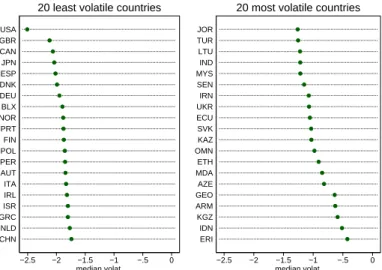
In Figure1, we depict the median of expenditure volatility (in logs) across destination markets
for the 20 least and most volatile countries over the 2000-2009 period.11 The United States
(US) has very low volatility, as do the UK and Canada (in the left panel). By contrast, the most volatile countries (in the right panel) tend to be developing countries. Our volatility measure confirms that, on average, developed countries are less volatile than developing countries, as
documented inWorld Bank(2013) andBloom(2014).
Figure 1: Least and most volatile countries
−2.5 −2 −1.5 −1 −.5 0 median volat. CHN NLD GRC ISR IRL ITA AUT PER POL FIN PRT NOR BLX DEU DNK ESP JPN CAN GBR USA
20 least volatile countries
−2.5 −2 −1.5 −1 −.5 0 median volat. ERI IDN KGZ ARM GEO AZE MDA ETH OMN KAZ SVK ECU UKR IRN SEN MYS IND LTU TUR JOR
20 most volatile countries
Note: This figure reports the median expenditure volatility (in logs) over the period 2000-2009 for the 20 least (left panel) and most (right panel) volatile countries.
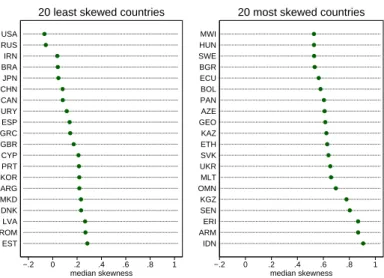
Similarly, Figure2reports the median skewness over the 2000-2009 period for the 20 least and
most skewed countries. Developed countries tend to be less skewed than developing countries,
as reported in Bekaert and Popov(2012). The difference between developed and developing
countries in terms of skewness seems, however, less pronounced than the difference in
volatil-ity.12 Two countries in our sample have negative median skewness: Russia and the US.
Expenditure volatility and skewness also vary across industries. Figure3 depicts the
distribu-tion of expenditure volatility (in logs) and skewness across 2-digit industries. The ranking of industries differs for the two moments. For example, the food and beverages category is among the most volatile industries, while its skewness is rather low. By contrast, the medical and op-11The distribution is computed for each destination using all 3-digit industries and years for which we are able to compute apparent consumption (we have, at most, 10 years * 57 three-digit industries = 570 observations per destination). We retain only countries for which we have at least 10% of the 570 possible observations.
12One limitation of our approach is that the number of industry-years for which we are able to compute volatility and skewness figures is smaller for developing countries than for developed countries, and this restriction may affect the median values.
Figure 2: Least and most skewed countries −.2 0 .2 .4 .6 .8 1 median skewness EST ROM LVA DNK MKD ARG KOR PRT CYP GBR GRC ESP URY CAN CHN JPN BRA IRN RUS USA
20 least skewed countries
−.2 0 .2 .4 .6 .8 1 median skewness IDN ARM ERI SEN KGZ OMN MLT UKR SVK ETH KAZ GEO AZE PAN BOL ECU BGR SWE HUN MWI
20 most skewed countries
Note: This figure reports the median skewness of expenditure over the period 2000-2009 for the 20 least (left panel) and the 20 most (right panel) skewed countries.
tical instruments industry has relatively low volatility but high skewness. Only two industries (tobacco; office, accounting) have negative median skewness.
Figure 3: Distribution of volatility and skewness, by industry
−4 −3 −2 −1 0 1 Other transport equipment
Machinery and equipment Radio, tv, comm. equipment coke, petroleum, nuclear fuel Medical, optical instruments Publishing, printing Fabricated metal products Furniture, manufacturing n.e.c Basic metals Electrical machinery Wood Motor vehicles Chemicals Leather Office, accounting Other mineral products Food & beverages Textiles Tobacco Wearing apparel Paper Rubber and plastics
Outside values excluded
Volatility, by industry
−2 0 2 4 Machinery and equipment
Other transport equipment Furniture, manufacturing n.e.c Publishing, printing Food & beverages Wood coke, petroleum, nuclear fuel Basic metals Other mineral products Wearing apparel Textiles Chemicals Fabricated metal products Motor vehicles Radio, tv, comm. equipment Medical, optical instruments Electrical machinery Leather Paper Rubber and plastics Office, accounting Tobacco
Outside values excluded
Skewness, by industry
Note: This figure reports the distribution of expenditure volatility (in logs) and skewness across 2-digit industries over the period 2000-2009.
A simple analysis of the variance of our volatility measure suggests that variations occur
pri-marily across countries and industries. Nevertheless, in accordance with the literature (Bloom,
2014), we also observe fluctuations in uncertainty over time. In particular, Figure4shows that
the mean volatility of food and beverage expenditures in the US increased between 2000 and 2008 (plain line). This finding confirms a trend that has been documented in the literature on US
food consumption (Gorbachev,2011).13 We also observe variation in the skewness distribution,
13Gorbachev(2011) shows that the mean volatility of household food consumption in the US increased between 1970 and 2004.
which is used for identification (dotted line).
Figure 4: Volatility and skewness of US expenditures on food and beverages, 2000-2008
-1
-.5
0
.5
1
Average expenditure skewness
-3
-2.8
-2.6
-2.4
-2.2
Average log of expenditure volatility
2000 2002 2004 2006 2008
year
Average log of expenditure volatility Average expenditure skewness
Role of Uncertainty: French Exports to Canada and Mexico
We provide some practical examples to illustrate the usefulness of our approach. Consider Canada and Mexico, which are characterized by similar levels of demand for some industries and are both seemingly distant markets in the American continent for French exporters. Let us pick three 3-digit industries for which total expenditures in 2005 are comparable in each country but risk exposure differs.
The first industry is chemical products (ISIC rev. 3 code 242). Expenditures are comparable in size (approximately 4 billion US dollars) and distribution (variance of 0.13 and skewness of -0.4) in both countries. It appears that the wedge between French export quantities to Mexico and to Canada is relatively low (12 and 15 million tons, respectively). This limited wedge could be explained by the same perceived risk exposure of French exporters in both countries.
By contrast, in the second industry (grain mill products and feeds; ISIC 153), expenditures in Canada and Mexico are similar (approximately 2 billion US dollars), but the volatility in Mexico is twice as high as that in Canada. Interestingly, the quantity of French exports to Canada is 2.6 times as high as exports to Mexico (11.7 and 5.4 million tons, respectively). In this case, for a given level of mean expenditures, managers appear to differentiate between Canada and Mexico, as the risk exposure of serving Mexico is higher.
Finally, managers can also be more sensitive to downside losses than to upside gains. For a given mean and variance, managers might prefer to serve a country exhibiting a high probability of an extreme event associated with a high or low level of demand. For instance, in the third industry (basic iron and steel; ISIC 271), expenditures in Canada and Mexico are similar (approximately 11 billion US dollars). However, the data show that the volatility is higher in Mexico than in Canada (0.38 and 0.22, respectively), whereas the skewness is positive in Mexico (1.83) and
negative in Canada (-0.14). Despite a slight difference in volatility, the difference in skewness may explain why the quantity of French exports to Mexico is higher than that to Canada (124 vs. 96 million tons, respectively). As Mexico exhibits a more right-skewed distribution in this industry, it can be viewed as providing better downside protection or lower downside risk, which induces more exports. Hence, for a given level of market potential, firms face different expenditure distributions and risk exposure, thereby inducing different levels of exports.
2.4. Empirical Evidence
We provide industry- and firm-level evidence of a significant effect of foreign expenditure volatility and skewness on exports.
2.4.1. Industry-level Evidence
This section presents our industry-level estimations on the intensive margin (export quantities by year) and extensive margin (number of firms per industry-destination-year) of trade.
Intensive Margin of Trade
We first estimate the following equation at the industry level:
ln qjtk = β1ln E(RKjt) + β2ln V(RKjt) + β3S(RKjt) + FE + εkjt, (2)
where qk
jt is the French export quantity to destination j aggregated at the 4-digit manufacturing
level k (ISIC classification) in year t. The sample covers the period from 2000 to 2009. Trade is related to the first three moments of the expenditure distribution of the destination and defined at the 3-digit level K: expected value E(RKjt), volatility V(RKjt), and skewness S(RKjt).14 FE is a
vector of different combinations of fixed effects, and εkjtrepresents the error term. The standard
errors are clustered at the destination-4-digit-industry level. We first consider industry (αk) and
destination-time (αjt) fixed effects, which control for unobserved heterogeneity in industries
and destination-year markets. These sets of fixed effects are selected according to a simple variance analysis suggesting that most of the variation in the volatility measure arises across
countries and industries. The results are reported in the first column of Table1.
Export quantities at the industry level are positively affected by the first and third central mo-ments of the foreign expenditure distribution, i.e., the expected expenditure and its skewness. The third-moment effect suggests that exporters are sensitive to downside risk exposure. In contrast, exports are negatively affected by the second central moment of expenditure. For
14Note that E(R
j) and V(Rj) are always positive, while S(Rj) can be either positive or negative. This explains
Table 1: Intensive and extensive margins: Industry export quantities and number of firms
Dependent variable: Industry export quantities: ln qk
jt Nb. of firms: ln nbkjt (1) (2) (3) (4) Ln Mean ExpenditureK jt 0.293a 0.293a 0.293a 0.118a (0.032) (0.032) (0.032) (0.012) Ln Expenditure VolatilityK jt -0.117a -0.078b -0.078b -0.084a (0.028) (0.031) (0.035) (0.011) Ln Expenditure VolatilityK jt× Ln Distancej 0.081a (0.022) Ln Expenditure VolatilityK jt× FTAj -0.101b (0.044) Expenditure SkewnessK jt 0.039a 0.040a 0.040a 0.019a (0.011) (0.011) (0.011) (0.004) Observations 47,858 47,858 47,858 47,858 R2 0.774 0.774 0.774 0.891
Sets of Fixed Effects:
Destination.Timejt Yes Yes Yes Yes
(4-digit-)Industryk Yes Yes Yes Yes
Notes: dependent variable is aggregated export quantities in logs (columns 1-3) and the number in logs of firms per (4-digit-)industry-destination-year triplet (column 4). Number of years: 10; Number of destinations: 90; Number of 4-digit industries: 119. Expenditure is defined as apparent consumption (production minus net exports) at the 3-digit K level. See the paper for computational details about expenditure moments. Distance is the geographical distance between France and the destination country. FTA includes all trade agreements in force between France and its trade partners. Robust standard errors are in parentheses, clustered by destination-4-digit industry level, withaandbdenoting significance at the 1% and 5%
level, respectively.
example, given that the export elasticity to expenditure volatility is 0.117, French exports to Canada in the grain mill industry would decrease by 11.7% if, ceteris paribus, its expenditure
were as volatile as that of Mexico.15
Columns 2 and 3 of Table1investigate whether the negative effect of expenditure volatility on
export quantities varies with trade barriers and trade policy in general. We know from Bloom
et al. (2007) that the responsiveness of investment to policy stimulus may be weaker in peri-ods of high uncertainty. We wonder whether the positive effects of trade policy on exports are weaker when expenditure uncertainty increases. The basic intuition is that the marginal nega-tive impact of volatility is magnified when market potential is higher. Thus, destination markets for which trade costs are low receive relatively more exports, which, in turn, implies a higher variance of profits. We use the geographical distance between France and the destination coun-try, as well as the free trade agreements (FTA) in force between France and its trade partners, to proxy for trade costs. In the regressions, we interact the volatility variable with distance (col-umn 2) and with the FTA dummy variable indicating whether at least one FTA with destination
j has been in force since 2000, the beginning of our sample period (column 3).16
15Recall that volatility in the grain mill products and feeds industry (ISIC rev. 3 code 153) is twice as high in Mexico as in Canada. See Section2.3.
16The distance to the destination country is obtained fromCEPIIand computed as the distance between the major cities of each country weighted by the share of the population living in each city. The data on FTA membership
Note that the separate effects of distance and FTA on French exports are captured by the destination-by-time fixed effects, which also absorb other time-variant and -invariant destina-tion covariates, such as a common language and contiguity. The estimated coefficient associated with the interaction term between volatility and distance is positive and significant at the one percent level. It also appears that FTAs significantly magnify the negative effect of expenditure volatility. In other words, higher expenditure uncertainty tends to shrink the positive impact of trade policy (lower trade barriers) on exports.
Extensive Margin of Trade
We now investigate the extensive margin of trade at the industry level and run the following estimation:
ln (nb firms)kjt = β1ln E(RKjt) + β2ln V(RjtK) + β3S(RKjt) + FE + ε k
jt, (3)
where (nb firms)kjt denotes the number (in logs) of French exporting firms in a
destination-(4-digit-)industry-year triplet. The number of French exporters is regressed on the first three mo-ments of the expenditure distribution of the destination at the 3-digit level K, E(RKjt), V(RKjt),
and S(RKjt). As previously, εkjt represents the error term, and the standard errors are clustered
at the destination-(4-digit-)industry level. The results reported in column 4 of Table 1control
for unobserved heterogeneity in industries and destination-year markets by including industry
(αk) and destination-time (αjt) fixed effects. The number of French exporters in a
destination-industry-year triplet is positively influenced by the expected demand and the skewness and negatively influenced by the volatility.
Heterogeneous Impact of Volatility on Exports
We supplement the analysis by presenting reduced-form graphical evidence of the heteroge-neous impact of volatility on exports. However, instead of using trade costs, we exploit differ-ences in productivity across firms. The intuition is similar to that presented above: the more pro-ductive the firm, the greater the export quantities and, therefore, the higher the risk at the margin.
Figure5compares the most to the least productive exporters in terms of industry export
quan-tities and expenditure volatility in destination markets between 2000 and 2009. Each industry-destination-year is binned based on the quartile of its expenditure volatility (x-axis), with bins from Q1 to Q4, where Q1 is the lowest and Q4 the highest quartile of volatility. The y-axis dis-plays the interquartile ratio of the 25% most productive firms to the 25% least productive firms in terms of the weighted average export quantities for each quartile of expenditure volatility. The weighted average export quantities are computed at the 4-digit industry-destination-year
level. The weights are the mean expenditures of the industry-destination-year triplets E(RKjt),
come fromDe Sousa(2012) (seehttp://jdesousa.univ.free.fr/data.htm). The countries with at least one FTA with France in force since 2000 are Eastern European countries, EU15 countries, Israel, Morocco, Norway, South Africa, Switzerland, Tunisia, and Turkey.
as defined in section2.2. They are designed to account for possible self-selection of firms into destinations with different levels of expenditure. The figure depicts an interesting and strik-ing result: expenditure volatility reduces the export difference between the least and the most productive exporters. The 25% most productive firms export, on average, 3.9 times more than the 25% least productive firms in less volatile markets (Q1), while this difference shrinks to 2.3 in the most volatile markets (Q4). Our theoretical model will rationalize this cautionary or “risk-averseness” effect.
Figure 5: Export difference in quantities between least and most productive exporters (Volatility in destination-year-industry markets – 2000-2009)
3.9 3.6 2.6 2.3 1 1.5 2 2.5 3 3.5 4
Interquartile ratio (75/25 productivity) of weighted average export volumes
Lowest (Q1) Highest (Q4)
Quartile of expenditure volatility in industry-destination markets
The figure compares most-to-least productive exporters in terms of export volumes and expenditure volatility in destination markets between 2000 and 2009: on average, the 25% most productive firms sell 3.9 times more than the 25% least productive ones in Q1 vs 2.3 in Q4. The x-axis displays the quartiles of expenditure volatility in 3-digit industry-destination-year triplets. The y-axis displays the interquartile ratio that compares the highest 25% of productive firms to the lowest 25% in terms of weighted average export volumes for each quartile of expenditure volatility. The weighted average export volumes are computed at the 4-digit industry-destination-year level. The weights are the lagged mean absorption of the industry-destination-year triplets.
by export volume and quartile of expenditure volatility
Comparing most-to-least productive exporters
2.4.2. Firm-level Evidence
We now present our firm-level estimations on the intensive and extensive margins of trade, i.e.,
on firm export sales and entry/exit decisions, respectively. Then, in Section2.5, we discuss the
economic meaningfulness of the estimates of volatility and skewness.
Intensive Margin of Trade
We estimate two intensive margins of trade: first on quantities and then on unit values.
Quantities. We estimate the following specification of firm-level export quantities at the destination-year-(4-digit-)industry triplet:
ln qf jtk = δ1ln E(RKjt) + δ2ln V(RKjt) + δ3S(RKjt) + FE + ε k
where qf jtk is now the export quantity of French firm f to destination j at the 4-digit manu-facturing level k in year t. As previously described, E(RKjt), V(RKjt), and S(RKjt) are the first
three central moments of the expenditure distribution, and εkf jtrepresents the usual error term.
Compared with the industry-level estimations, firm-level data offer considerably more obser-vations and mitigate concerns about the inefficiency of the panel estimator when introducing various combinations of fixed effects. Consequently, we use fairly demanding specifications with a vector FE of different combinations of fixed effects. The standard errors are clustered at the destination-4-digit-industry level.17
The results are reported in Table 2 according to the main source of variation in expenditure:
across destination markets (column 1), industries (column 2), and years (column 3). Before discussing the differences across columns, note that in every specification, all coefficients are statistically significant (at the 1 percent confidence level) and exhibit the expected signs. The results clearly show that expenditure volatility is negatively correlated with firm export quan-tities. This confirms the industry evidence presented above. Moreover, as expected, average expenditures, skewness, and firm productivity are positively correlated with the export quanti-ties.
In the first column, we introduce firm-by-industry-by-year fixed effects (αf kt), which capture
all time-varying specific determinants, such as productivity and debt, as well as any firm-industry heterogeneity. The coefficients of interest on volatility and skewness are identified in the destination dimension. In other words, the estimation relies on firm-industry-year triplets
with multiple destinations. We add a separate destination-country fixed effect (αj) to control for
destination-specific factors. In this way, we investigate whether multi-destination firms favor countries with low volatility and high skewness. That is, this estimation neutralizes the ability of firms to manage their risk exposure by adjusting their (4-digit) product lines.
In this fixed effects setting, we find a negative effect of expenditure volatility and a positive effect of expenditure skewness on firm-level exports. Hence, multi-destination firms manage
their risk exposure by favoring countries with low expenditure variance and high skewness.18
In other words, firms avoid a high-risk market j by diverting exports to other markets with lower risk.
In the second column, we introduce firm-by-destination-by-year fixed effects (αf jt). With this
specification, we still absorb productivity differences across firms, but we also control for any time-varying firm-destination-specific factors. Our coefficients of interest are now identified in 17We use the Stata package REGHDFE developed byCorreia(2014). Because maintaining singleton groups in linear regressions where fixed effects are nested within clusters might lead to incorrect inferences, we exclude groups containing only one observation (Correia,2015). Therefore, the number of observations differs across estimations. The results are similar when retaining singleton groups and are available upon request.
18Note that restricting the estimations to multi-destination and -industry exporters only marginally affects the estimates. These results are available upon request.
Table 2: Intensive margin: Firm export quantities
Dependent variable: Firm export quantities: ln qk f jt (1) (2) (3) Ln Mean ExpenditureK jt 0.068a 0.079a 0.200a (0.018) (0.022) (0.030) Ln Expenditure VolatilityK jt -0.028a -0.040a -0.024a (0.009) (0.012) (0.008) Expenditure SkewnessK jt 0.012a 0.015a 0.009a (0.004) (0.005) (0.003) Ln Productivityf t - - 0.123a (0.004) Observations 3,904,513 3,129,051 3,875,422 R2 0.708 0.534 0.861
Sets of Fixed Effects:
Firm.(4-digit-)Industry.Timef kt Yes - -Destinationj Yes - -Firm.Destination.Timef jt - Yes -(4-digit-)Industryk - Yes -Firm.Destination.(4-digit-)Industryf jk - - Yes Timet - - Yes
Notes: dependent variable is firm-level export quantities in logs aggregated at the 4-digit k level. Number of years: 10; Number of destinations: 90; Number of 4-4-digit industries: 119; Number of firms: 105,777. Expenditure is defined as apparent con-sumption (production minus net exports) at the 3-digit K level. See the paper for computational details about expenditure moments. Robust standard errors are in paren-theses, clustered by destination-4-digit industry level, withadenoting significance at
the 1% level.
the industry dimension. In other words, the estimation relies on firm-destination-year triplets
with multiple 4-digit industries. We add a separate 4-digit industry fixed effect (αj) to control
for industry-specific factors. Hence, we estimate whether firms favor the exports of industries with low volatility and high skewness for a given firm-destination-year triplet. In this setting, by controlling for firm-by-destination-by-year fixed effects, we eliminate the possibility that firms diversify across destinations. Unsurprisingly, the magnitude of the volatility estimate increases (from 0.028 in column 1 to 0.040 in column 2). Firms are more affected because it is intuitively more difficult to diversify across industries than across destinations when uncertainty increases. The magnitude of the skewness effect is also somewhat larger.
In the third column, we use firm-by-destination-by-industry fixed effects (αf jk) and add a
sepa-rate year fixed effect (αt). We capture any differences that are maintained across our observation
period at the firm-destination-industry level. However, this set does not control for time-varying firm characteristics such as productivity, which is now introduced as an additional control and defined as the ratio of value added to the number of employees. The estimates in the third col-umn have a very natural interpretation with a set of fixed effects corresponding to a within-panel estimator. The identification lies in the variation of expenditure moments over time. The within estimates suggest that, for a given firm-destination-industry triplet, an increase in volatility over time reduces the firm’s export quantities, while an increase in skewness increases exports.
Table7of AppendixBtests the robustness of our results by considering alternative time spans for the construction of the expenditure moments. Instead of using a 6-year time window, volatil-ity and skewness are calculated over 5-year and 7-year rolling periods, respectively. The results for firm-export quantities are robust to these alternatives, and the previous conclusions remain unchanged.
Prices. We now check whether the three moments of the expenditure distribution influence prices. We estimate the following specification for firm-level export prices for destination-year-(4-digit-)industry triplets: ln pkf jt= δ1ln E(RKjt) + δ2ln V(RKjt) + δ3S(RKjt) + quality k f jt+ FE + ε k f jt, (5)
where pkf jt is now the export price of French firm f to destination j at the 4-digit
manufactur-ing level k in year t. E(RKjt), V(RKjt), and S(RKjt) are the first three central moments of the expenditure distribution, and εkf jtis the usual error term. Prices pkf jt are proxied by unit values and defined as the ratio of export value to export quantity. Unit values are known to include a quality component in addition to productivity. More productive firms have lower marginal costs but may export at higher prices due to quality. Omitting the quality component may reverse the empirical conclusions. We account for potential contamination of prices by quality by using the
strategy ofKhandelwal et al. (2013). For a given price in an industry(4-digit)-destination-year
triplet, a variety with a higher quantity is assigned a higher quality. Qualityk
f jt is thus esti-mated for each firm-industry-destination-year observation as the residual of the following OLS regression:
ln qkf jt+ lnpe k
f jt = αjt+ αk+ εkf jt, (6) where qkf jtis the export quantity,pe
k
f jtis the substitution-adjusted export price,19 αjt and αk are destination-year and industry (4-digit) fixed effects, respectively.
The results are reported in Table 3 according to the same source of variation in expenditure
used in Table 2: destination markets (column 1), industries (column 2), and years (column 3).
As expected, quality is positively correlated with prices. The first and third central expenditure moments are also positively correlated with prices, while a negative correlation is observed for the second moment. A plausible and coherent explanation for the expenditure moment estimates is linked to the risk premium and to pro-competitive effects. For instance, the higher the demand and skewness, the higher the competition in the market, and thus, the lower the price. By contrast, the higher the volatility, the higher the risk premium, the lower the competition, and the higher the price. Furthermore, in column 3, controlling for the quality and expenditure
19InKhandelwal et al.(2013), the left-hand side variable of equation (6) is equal to ln qk
f jt+ σ ln p k
f jt, where σ
is the elasticity of substitution such thatepk f jt= p
k f jtexp
σ. Quality is estimated as qualityk
f jt= ˆεkf jt/(σ − 1) using
moments, an increase in productivity implies a lower marginal cost and a price decrease. Our results suggest that decision makers care about expenditure uncertainty when they decide the quantity to export or the prices.
Table 3: Intensive margin: Firm export prices
Dependent variable: Firm export prices: ln pk f jt (1) (2) (3) Ln Mean ExpenditureK jt -0.017 a -0.017a -0.062a (0.004) (0.005) (0.009) Ln Expenditure VolatilityK jt 0.005 b 0.009a 0.004 (0.002) (0.003) (0.002) Expenditure SkewnessK jt -0.003 a -0.004a -0.002a (0.001) (0.001) (0.001) Ln Qualityf jkt 0.644a 0.640a 0.750a (0.003) (0.003) (0.002) Ln Productivityf t - - -0.030a - - (0.001) Observations 3,904,513 3,129,051 3,875,422 R2 0.945 0.917 0.973
Sets of Fixed Effects:
Firm.(4-digit-)Industry.Timef kt Yes - -Destinationj Yes - -Firm.Destination.Timef jt - Yes -4-digit-Industryk - Yes -Firm.destination.(4-digit-)Industryf jk - - Yes Timet - - Yes
Notes: dependent variable is firm-level export unit values in logs aggregated at the digit k level. Number of years: 10; Number of destinations: 90; Number of 4-digit industries: 119; Number of firms: 105,777. Expenditure is defined as apparent consumption (production minus net exports) at the 3-digit K level. See the paper for computational details about expenditure moments. Qualityf jktis computed using
Khandelwal et al.(2013)’s approach. The productivity of firm f in year t is measured using the value-added per employee. Robust standard errors are in parentheses, clus-tered by destination-4-digit industry level, witha,bdenoting significance at the 1%
and 5% level respectively.
Heterogeneous Intensive Responses of Firms to Expenditure Volatility
In this section, we assess the potential for heterogeneity in firm responses to volatility. Specif-ically, we evaluate whether expenditure uncertainty reduces the export difference between the
least and the most productive firms, as depicted in the non-parametric Figure5. In Figure6, we
Figure 6: Volatility, productivity and export quantities -.85 -.8 -.75 -.7 -.65 -.6 -.55
Predicted mean export quantity (in logs)
Low (D1) Med (D5) Hi (D9)
Decile of expenditure volatility in industry-destinations
Ln(prod) >= P(75) P(50) <= Ln(prod) < P(75) P(25) <= Ln(prod) < P(50) Ln(prod) < P(25) Firm Productivity Quartile:
Notes: The figure compares exporters across categories of productivity (prod) and expenditure volatility in terms of predicted export quantities between 2000 and 2009. The x-axis displays the deciles of expenditure volatility in 3-digit industry-destination-year triplets. The y-axis displays the predicted mean export quantity in 4-digit industry-destination-year triplets. See the text for estimation details.
Predictive margins with 95% confidence intervals
We first divide firm productivity into quartiles and industry expenditure volatility into deciles. Then, we create new variables by interacting each productivity quartile with the volatility deciles. Finally, we use an estimator that allows us to identify these interactions and to overcome the computational cost of calculating marginal effects. We run the regression by conditioning
firm responses on the destination-by-year and firm-by-industry (4-digit) fixed effects.20 Based
on the estimated parameters, we compute the predicted mean of export quantity (in logs) for each decile of volatility and quartile of productivity. The different predictions for trade are
plotted in Figure6. This plot shows three interesting results: (1) the most productive firms
ex-port more than the others at any level of volatility; (2) the greater the expenditure volatility, the smaller the export quantities for all levels of productivity, except for the least productive firms; and (3) the marginal decrease in exports increases for the most productive firms as volatility in-creases. These results imply that the export difference between the least and the most productive firms decreases with volatility.
We pursue our investigation of the heterogeneous responses of firms to expenditure volatility
us-ing the same specifications as in Table2and a new covariate: the interaction between volatility
and firm productivity. The results are reported in Table4. Our estimates confirm that the most
productive firms are more sensitive to variation in expenditure volatility (across destinations, 20Note that this estimator yields the same estimates of volatility and skewness as those presented in column 3 of Table2without the interactions.
industries, and years).
Table 4: Intensive margin: Reallocation of export quantities across firms
Dependent variable: Firm export quantities: ln qk
f jt (1) (2) (3) Ln Mean ExpenditureK jt 0.065 a 0.078a 0.200a (0.018) (0.021) (0.030) Ln Expenditure VolatilityK jt 0.008 -0.017 -0.011 (0.010) (0.012) (0.008) Ln VolatilityK jt× Ln Productivityf t -0.011a -0.007a -0.004a (0.002) (0.001) (0.001) Expenditure SkewnessK jt 0.012 a 0.015a 0.009a (0.004) (0.005) (0.003) Ln Productivityf t - - 0.117a (0.004) Observations 3,904,513 3,129,051 3,8754,22 R2 0.708 0.534 0.861
Sets of Fixed Effects:
Firm.(4-digit-)Industry.Timef kt Yes - -Destinationj Yes - -Firm.Destination.Timef jt - Yes -(4-digit-)Industryk - Yes -Firm.Destination.(4-digit-)Industryf jk - - Yes Timet - - Yes
Notes: dependent variable is firm-level export quantities in logs aggregated at the 4-digit
k level. All specifications include the overall sample of exporters. Number of years: 10;
Number of destinations: 90; Number of 4-digit industries: 119; Number of firms: 105,777. Expenditure is defined as apparent consumption (production minus net exports) at the 3-digit K level. See the paper for computational details about expenditure moments. The productivity of firm f in year t is measured using the value-added per employee. Robust standard errors are in parentheses, clustered by destination-4-digit industry level, witha
denoting significance at the 1% level.
Extensive Margin of Trade
We now investigate the impact of uncertainty on the extensive margin of trade. We follow the same identification strategy as above with a disaggregated left-hand side variable regressed on aggregated right-hand side expenditure moments. We distinguish between the entry of new French firms into the international market and the exit of incumbents from that market over the
2000-2009 period. Regarding entry, our dependent variable (yf jtk ) is the probability that firm f
begins exporting to destination j in 4-digit industry k and year t. Our counterfactual scenario considers the firms that do not enter in the same triplet jkt. This choice model can be written
as a latent variable representation, with y∗kf jt being the latent variable that determines whether
a strictly positive export flow is observed for firm f in a destination-industry-year triplet. Our estimated equation is therefore:
P r(yf jtk |yk f j,t−1 = 0) = 1 if y∗kf jt> 0, 0 if y∗kf jt≤ 0, (7) with yf jt∗k = γ1ln E(RKj,t−1) + γ2ln V(RKjt) + γ3S(RKjt) + FE + ε k f jt,
where, as previously described, E(RKjt), V(RjtK), and S(RKjt) are the first three central moments
of the expenditure distribution, FE represents various combinations of fixed effects, and εkf jtis
the error term. In addition to the probability of entry, one can study the exit transition. Higher volatility or lower upside gains may indeed increase the exit of firms from the export market. In that case, our dependent variable is the probability that firm f in destination j, industry
k and year t − 1 stops exporting products from industry k to this destination in year t. Our
counterfactual scenario now considers the firms that continue to serve the same triplet jkt. The explanatory variables are the same as in the entry estimations.
We estimate the entry and exit equations using a linear probability model (LPM). The inclusion of fixed effects in a probit model would give rise to the incidental parameter problem. The LPM avoids this issue. Furthermore, the use of an LPM allows us to directly interpret the coefficients. As for the intensive margin, in all regressions, we account for the correlation of
errors by clustering at the destination-4-digit-industry level. The results are reported in Table5.
In accordance with the definition of our counterfactual scenarios, we investigate the effects of uncertainty across industries and destinations. In columns 1 and 3, we introduce destination
(αj) and firm-by-industry-by-year fixed effects (αf kt). Here, our coefficients of interest on
volatility and skewness are identified in the destination dimension. In other words, regarding the probability of firm entry (column 1), we compare firms in a given industry k and year t entering an export market j versus those that are not entering that market. In columns 2 and 4,
we introduce industry (αk) and firm-by-destination-by-year fixed effects (αf jt). Our coefficients
of interest on volatility and skewness are now identified in the industry dimension. Regarding the probability of firm entry (column 3), we thus compare firms in a given destination j and year t entering industry k versus those that are not entering that industry.
Table 5 presents quite intuitive results. The average expenditure significantly increases the
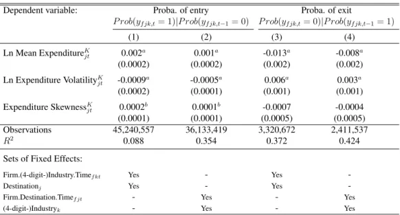
probability that a firm enters a destination j or an industry k, while reducing the probability of exit (columns 3 and 4). As expected, the within industry-time (columns 1 and 3) and firm-destination-time (columns 3 and 4) dimensions react to the second- and third-order moment changes in expenditures. Expenditure volatility significantly decreases the probability of entry and increases the probability of exit. These results depict reallocation effects across destinations and industries in terms of export decisions. Interestingly, destination reallocation appears to be stronger (see columns 1 and 3 vs. columns 2 and 4). As noted for the intensive margin of trade, diversification and reallocation across destinations is easier than diversification across industries, which may explain the difference in the magnitudes of the coefficients. Thus, a smaller volatility effect on the intensive margin is consistent with a larger effect on the extensive margin. Note that skewness has a positive and significant impact on the probability of entry but no exit effect.
Table 5: Extensive margin: Firm entry and exit probabilities
Dependent variable: Proba. of entry Proba. of exit
P rob(yf jk,t= 1)|P rob(yf jk,t−1= 0) P rob(yf jk,t= 0)|P rob(yf jk,t−1= 1)
(1) (2) (3) (4) Ln Mean ExpenditureK jt 0.002a 0.001a -0.013a -0.008a (0.0002) (0.0002) (0.002) (0.002) Ln Expenditure VolatilityK jt -0.0009 a -0.0005a 0.006a 0.003a (0.0002) (0.0001) (0.001) (0.001) Expenditure SkewnessK jt 0.0002b 0.0001b -0.0007 -0.0004 (0.0001) (0.0001) (0.0005) (0.0005) Observations 45,240,557 36,133,419 3,320,672 2,411,537 R2 0.088 0.354 0.372 0.424
Sets of Fixed Effects:
Firm.(4-digit-)Industry.Timef kt Yes - Yes
-Destinationj Yes - Yes
-Firm.Destination.Timef jt - Yes - Yes
(4-digit-)Industryk - Yes - Yes
Notes: dependent variable is probability for a firm to enter the export market (columns 1-2) and probability for a firm to exit the export market (columns 3-4). Entry sample: 9 years, 89 destinations, 119 4-digit industries, and 74,575 firms. Exit sample: 9 years, 88 destinations, 119 4-digit industries, and 72,694 firms. Expenditure is defined as apparent consumption (production minus net exports) at the 3-digit K level. See the paper for computational details about expenditure moments. Robust standard errors are in parentheses, clustered by destination-4-digit industry level, witha,bdenoting significance at the 1% and 5% level respectively.
We check the robustness of our results in Table 8of AppendixCby selecting alternative time
spans for the construction of the expenditure moments (5- and 7-year rolling periods instead of
a 6-year time window). The results are similar to those reported in Table5and are therefore not
driven by the time span chosen for the expenditure moments.
2.5. Discussion and Simulations
Our estimations reveal that expenditure volatility negatively affects the intensive and extensive margins of trade. In addition, more productive firms seem to favor destinations or industries with low volatility. In contrast, low productivity exporters can increase their exports in the riskiest countries or industries due to the reallocation of market shares among firms. Our results also suggest that downside risk matters to exporters.
How economically meaningful are the estimates of volatility and skewness? The firm-level esti-mates are our preferred estiesti-mates. Compared with the industry-level estimations, the number of firm-level observations improves the efficiency of the panel estimator when various combina-tions of fixed effects are introduced. Nevertheless, the firm-level estimates likely underestimate the magnitude of the effects. Indeed, our estimations only consider variation along a single di-mension (destination, industry, or time), whereas our measures of volatility and skewness vary
along the three dimensions (see Section 2.3). In addition, our simulations focus only on the
intensive margin, disregarding the effects on the extensive margin. Our simulations also neglect feedback effects on price and demand. As a result, the magnitude of the positive effect of lower uncertainty can be viewed as a minimum threshold.