HAL Id: cea-02327633
https://hal-cea.archives-ouvertes.fr/cea-02327633
Submitted on 22 Oct 2019
HAL is a multi-disciplinary open access
archive for the deposit and dissemination of
sci-entific research documents, whether they are
pub-lished or not. The documents may come from
teaching and research institutions in France or
abroad, or from public or private research centers.
L’archive ouverte pluridisciplinaire HAL, est
destinée au dépôt et à la diffusion de documents
scientifiques de niveau recherche, publiés ou non,
émanant des établissements d’enseignement et de
recherche français ou étrangers, des laboratoires
publics ou privés.
Estimating the galaxy two-point correlation function
using a split random catalog
E. Keihänen, H. Kurki-Suonio, V. Lindholm, A. Viitanen, A.-S. Suur-Uski, V.
Allevato, E. Branchini, F. Marulli, P. Norberg, D. Tavagnacco, et al.
To cite this version:
E. Keihänen, H. Kurki-Suonio, V. Lindholm, A. Viitanen, A.-S. Suur-Uski, et al.. Estimating the
galaxy twopoint correlation function using a split random catalog. Astronomy and Astrophysics
-A&A, EDP Sciences, 2019, 631, pp.A73. �10.1051/0004-6361/201935828�. �cea-02327633�
https://doi.org/10.1051/0004-6361/201935828 c ESO 2019
Astronomy
&
Astrophysics
Estimating the galaxy two-point correlation function using a split
random catalog
E. Keihänen
1, H. Kurki-Suonio
1, V. Lindholm
1, A. Viitanen
1, A.-S. Suur-Uski
1, V. Allevato
2,1, E. Branchini
3,
F. Marulli
4,5,6, P. Norberg
7, D. Tavagnacco
8, S. de la Torre
9, J. Valiviita
1, M. Viel
10,11,8,14, J. Bel
12,
M. Frailis
8, and A. G. Sánchez
131 Department of Physics and Helsinki Institute of Physics, University of Helsinki, Gustaf Hällströmin katu 2, 00014 Helsinki,
Finland
e-mail: [email protected]
2 Scuola Normale Superiore, Piazza dei Cavalieri 7, 56126 Pisa, Italy
3 Department of Mathematics and Physics, Roma Tre University, Via della Vasca Navale 84, 00146 Rome, Italy
4 Dipartimento di Fisica e Astronomia – Alma Mater Studiorum Università di Bologna, Via Piero Gobetti 93/2, 40129 Bologna,
Italy
5 INAF – Osservatorio di Astrofisica e Scienza dello Spazio di Bologna, Via Piero Gobetti 93/3, 40129 Bologna, Italy 6 INFN – Sezione di Bologna, Viale Berti Pichat 6/2, 40127 Bologna, Italy
7 ICC & CEA, Department of Physics, Durham University, South Road, Durham DH1 3LE, UK 8 INAF, Osservatorio Astronomico di Trieste, Via Tiepolo 11, 34131 Trieste, Italy
9 Aix Marseille Univ., CNRS, CNES, LAM, Marseille, France
10 SISSA, International School for Advanced Studies, Via Bonomea 265, 34136 Trieste, TS, Italy 11 INFN, Sezione di Trieste, Via Valerio 2, 34127 Trieste, TS, Italy
12 Aix Marseille Univ., Université de Toulon, CNRS, CPT, Marseille, France
13 Max-Planck-Institut für Extraterrestrische Physik, Postfach 1312, Giessenbachstr., 85741 Garching, Germany 14 IFPU – Institute for Fundamental Physics of the Universe, Via Beirut 2, 34014 Trieste, Italy
Received 3 May 2019/ Accepted 24 July 2019
ABSTRACT
The two-point correlation function of the galaxy distribution is a key cosmological observable that allows us to constrain the dynamical and geometrical state of our Universe. To measure the correlation function we need to know both the galaxy positions and the expected galaxy density field. The expected field is commonly specified using a Monte-Carlo sampling of the volume covered by the survey and, to minimize additional sampling errors, this random catalog has to be much larger than the data catalog. Correlation function estimators compare data–data pair counts to data–random and random–random pair counts, where random–random pairs usually dominate the computational cost. Future redshift surveys will deliver spectroscopic catalogs of tens of millions of galaxies. Given the large number of random objects required to guarantee sub-percent accuracy, it is of paramount importance to improve the efficiency of the algorithm without degrading its precision. We show both analytically and numerically that splitting the random catalog into a number of subcatalogs of the same size as the data catalog when calculating random–random pairs and excluding pairs across different subcatalogs provides the optimal error at fixed computational cost. For a random catalog fifty times larger than the data catalog, this reduces the computation time by a factor of more than ten without affecting estimator variance or bias.
Key words. large-scale structure of Universe – cosmology: observations – methods: statistical – methods: data analysis
1. Introduction
The spatial distribution of luminous matter in the Universe is a key diagnostic for studying cosmological models and the physi-cal processes involved in the assembly of structure. In particular, light from galaxies is a robust tracer of the overall matter distri-bution, whose statistical properties can be predicted by cosmo-logical models. Two-point correlation statistics are very effective tools for compressing the cosmological information encoded in the spatial distribution of the mass in the Universe. In particu-lar, the two-point correlation function in configuration space has emerged as one of the most popular cosmological probes. Its suc-cess stems from the presence of characterized features that can be identified, measured, and effectively compared to theoretical models to extract clean cosmological information.
One such feature is baryon acoustic oscillations (BAOs), which imprint a characteristic scale in the two-point correlation
function that can be used as a standard ruler. After the first detection in the two-point correlation function of SDSS DR3 and 2dFGRS galaxy catalogs (Eisenstein et al. 2005;Cole et al. 2005), the BAO signal was identified, with different degrees of statistical significance, and has since been used to constrain the expansion history of the Universe in many spectroscopic galaxy samples (see e.g.,Percival et al. 2010;Blake et al. 2011;
Beutler et al. 2011;Anderson et al. 2012,2014;Ross et al. 2015,
2017; Alam et al. 2017; Vargas-Magaña et al. 2018; Bautista et al. 2018;Ata et al. 2018). Several of these studies did not focus on the BAO feature only but also analyzed the anisotropies in the two-point correlation function induced by the peculiar veloci-ties (Kaiser 1987), the so-called redshift space distortions (RSD), and by assigning cosmology-dependent distances to the observed redshifts (theAlcock & Paczy´nski 1979test). For RSD analyses, see also, for example,Peacock et al.(2001),Guzzo et al.(2008),
Pezzotta et al.(2017),Zarrouk et al.(2018),Hou et al.(2018), andRuggeri et al.(2019).
Methods to estimate the galaxy two-point correlation func-tion (2PCF) ξ(r) from survey data are based on its definifunc-tion as the excess probability of finding a galaxy pair. One counts from the data (D) catalog the number DD(r) of pairs of galaxies with separation x2−x1∈r, where r is a bin of separation vectors, and
compares it to the number of pairs RR(r) in a corresponding ran-domly generated (R) catalog and to the number of data-random pairs DR(r). The bin may be a 1D (r ±12∆r), 2D, or a 3D bin. In the 1D case, r is the length of the separation vector and∆r is the width of the bin. From here on, “separation r” indicates that the separation falls in this bin.
Several estimators of the 2PCF have been proposed by
Hewett(1982),Davis & Peebles(1983),Hamilton(1993), and
Landy & Szalay (1993), building on the original Peebles & Hauser(1974) proposal. These correspond to different combina-tions of the DD, DR, and RR counts to obtain a 2PCF estimate
ˆ
ξ(r); seeKerscher(1999) andKerscher et al.(2000) for more esti-mators. The Landy–Szalay (Landy & Szalay 1993) estimator
ˆ ξLS(r) := N0 r(Nr0− 1) Nd(Nd− 1) DD(r) RR(r) − N0 r− 1 Nd DR(r) RR(r) + 1, (1) (we call this method “standard LS” in the following) is the most commonly used, since it provides the minimum variance when |ξ| 1 and is unbiased in the limit N0
r → ∞. Here Ndis the size
(number of objects) of the data catalog and Nr0is the size of the
random catalog. We define Mr := Nr0/Nd. To minimize random
error from the random catalog, Mr 1 should be used (for a
different approach, seeDemina et al. 2018).
One is usually interested in ξ(r) only up to some rmax Lmax
(the maximum separation in the survey), and therefore pairs with larger separations can be skipped. Efficient implementations of the LS estimator involve pre-ordering of the catalogs through kd-tree, chain-mesh, or other algorithms (e.g., Moore et al. 2000;
Alonso 2012;Jarvis 2015;Marulli et al. 2016) to facilitate this. The computational cost is then roughly proportional to the actual number of pairs with separation r ≤ rmax.
The correlation function is small for large separations, and in cosmological surveys rmax is large enough so that for most
pairs |ξ(r)| 1. The fraction f of DD pairs with r ≤ rmax is
therefore not very different from the fraction of DR or RR pairs with r ≤ rmax. The computational cost is dominated by the part
proportional to the total number of pairs needed,12f Nd(Nd− 1)+
f NdNr+12f Nr0(Nr0− 1) ≈ 12f N 2
d(1+ 2Mr+ M 2
r), which in turn
is dominated by the RR pairs as Mr 1. The smaller number
of DR pairs contribute much more to the error of the estimate than the large number of RR pairs, whereas the cost is dominated by RR. Thus, a significant saving of computation time with an insignificant loss of accuracy may be achieved by counting only a subset of RR pairs, while still counting the full set (up to rmax)
of DR pairs.
A good way to achieve this is to use many small (i.e, low-density) R catalogs instead of one large (high-density) cat-alog (Landy & Szalay 1993;Wall & Jenkins 2012;Slepian & Eisenstein 2015), or, equivalently, to split an already generated large R catalog into Mssmall ones for the calculation of RR pairs
while using the full R catalog for the DR counts. This method has been used by some practitioners (e.g.,Zehavi et al. 20111), but this is usually not documented in the literature. One might also consider obtaining a similar cost saving by diluting (sub-sampling) the R catalog for RR counts, but, as we show below,
1 I. Zehavi, priv. comm.
this is not a good idea. We refer to these two cost-saving methods as “split” and “dilution”.
In this work we theoretically derive the additional covari-ance and bias due to the size and treatment of the R catalog; test these predictions numerically with mock catalogs representa-tive of next-generation datasets, such as the spectroscopic galaxy samples that will be obtained by the future Euclid satellite mis-sion (Laureijs et al. 2011); and show that the “split” method, while reducing the computational cost by a large factor, retains the advantages of the LS estimator.
We follow the approach ofLandy & Szalay(1993; hereafter, LS93), but generalize it in a number of ways: In particular, since we focus on the effect of the random catalog, we do not work in the limit Mr → ∞. Also, we calculate covariances, not just
variances, and make fewer approximations (see Sect.2.2). The layout of the paper is as follows. In Sect. 2we derive theoretical results for bias and covariance. In Sect.3 we focus on the split LS estimator and its optimization. In Sect.4we test the different estimators with mock catalogs. Finally, we discuss the results and present our conclusions in Sect.5.
2. Theoretical results: bias and covariance
2.1. General derivation
We follow the derivation and notations in LS93 but extend to the case that includes random counts covariance. We consider the survey volume as divided into K microcells (very small subvol-umes) and work in the limit K → ∞, which means that no two objects will ever be located within the same microcell.
Here, α, β, and γ represent the relative deviation of the DD(r), DR(r), and RR(r) counts from their expectation values (mean values over an infinite number of independent realiza-tions):
DD(r)=: hDD(r)i[1 + α(r)], DR(r)=: hDR(r)i[1 + β(r)],
RR(r)=: hRR(r)i[1 + γ(r)]. (2)
By definition hαi = hβi = hγi = 0. The factors α, β, and γ rep-resent fluctuations in the pair counts, which arise as a result of a Poisson process. As long as the mean pair counts per bin are large ( 1) the relative fluctuations will be small. We calculate up to second order in α, β, and γ, and ignore the higher-order terms (in the limit Mr→ ∞, γ → 0, so LS93 set γ= 0 at this point).
The expectation values for the pair counts are: hDD(r)i=1 2Nd(Nd− 1)G p(r)[1+ ξ(r)], hDR(r)i= NdNrGp(r), hRR(r)i=1 2N 0 r(N 0 r − 1)G p(r), (3)
where ξ(r) is the correlation function normalized to the actual number density of galaxies in the survey and
Gp(r) := 2 K2 K X i< j Θi j(r) (4)
is the fraction of microcell pairs with separation r. HereΘi j(r) :=
1 if xi−xjfalls in the r-bin, otherwise it is equal to zero.
The expectation value of the LS estimator (1) is h ˆξLSi= (1 + ξ) * 1+ α 1+ γ + − 2* 1+ β 1+ γ + + 1 h ξ + (ξ − 1)hγ2i+ 2hβγi. (5)
A finite R catalog thus introduces a (small) bias. (In LS93, γ = 0, so the estimator is unbiased in this limit). This expression is calculated to second order in α, β, and γ (we denote equality to second order by “h”). Calculation to higher order is beyond the scope of this work. Since data and random catalogs are inde-pendent, hαγi= 0.
We introduce shorthand notations hα1α2i for hα(r1)α(r2)i,
hDD1DD2i for hDD(r1)DD(r2)i, and similarly for other terms.
For the covariance we get Covh ˆξLS(r1), ˆξLS(r2) i ≡D ˆξLS(r1) ˆξLS(r2) E −D ˆξLS(r1)E D ˆξLS(r2) E h (1 + ξ1)(1+ ξ2)hα1α2i+ 4hβ1β2i + (1 − ξ1)(1 − ξ2)hγ1γ2i − 2(1+ ξ1)hα1β2i − 2(1+ ξ2)hβ1α2i − 2(1 − ξ1)hγ1β2i − 2(1 − ξ2)hβ1γ2i. (6) Terms with γ represent additional variance due to finite N0
r, and
are new compared to those of LS93. Also, hβ1β2i collects an
additional contribution, which we denote by∆hβ1β2i, from
vari-ations in the random field (see Sect.2.3). The cross terms α1β2
and α2β1, instead depend linearly on the random field, and
aver-age to the N0
r → ∞ result. The additional contribution due to
finite N0 r is thus ∆Covh ˆξLS(r1), ˆξLS(r2)i h 4∆hβ1β2i+ (1 − ξ1)(1 − ξ2)hγ1γ2i − 2(1 − ξ1)hγ1β2i − 2(1 − ξ2)hβ1γ2i. (7) From (2), hDD1DD2i= hDD1ihDD2i(1+ hα1α2i), (8)
and so on, so that the covariances of the deviations are obtained from hα1α2i=hDD1DD2i − hDD1ihDD2i hDD1ihDD2i , hβ1β2i= hDR1DR2i − hDR1ihDR2i hDR1ihDR2i , hγ1γ2i= hRR1RR2i − hRR1ihRR2i hRR1ihRR2i , hα1β2i= hDD1DR2i − hDD1ihDR2i hDD1ihDR2i , hβ1γ2i= hDR1RR2i − hDR1ihRR2i hDR1ihRR2i , hα1γ2i= hDD1RR2i − hDD1ihRR1i hDD1ihRR2i = 0. (9)
2.2. Quadruplets, triplets, and approximations We use Gt12:= Gt(r1, r2) := 1 K3 ∗ X i jk Θik 1Θ jk 2 (10)
to denote the fraction of ordered microcell triplets, where xi−
xk∈r1and xj−xk∈r2. The notationP∗means that only terms
where all indices (microcells) are different are included. Here Gt
12is of the same magnitude as G p 1G
p
2but is larger.
AppendixAgives examples of how the hDD1 DD2i and so
on in (9) are calculated. These covariances involve expectation values hninjnlnki, where ni is the number of objects (0 or 1)
in microcell i and so on, and only cases where the four micro-cells are separated pairwise by r1and r2are included. If all four
microcells i, j, k, and l are different, we call this case a quadru-plet; it consists of two pairs with separations r1and r2. If two of
the indices, that is, microcells, are equal, we have a triplet with a center cell (the equal indices) and two end cells separated from the center by r1and r2.
We make the following three approximations:
1. For microcell quadruplets, the correlations between uncon-nected cells are approximated by zero on average.
2. Three-point correlations vanish.
3. The part of four-point correlations that does not arise from the two-point correlations vanishes.
With approximations (2) and (3), we have for the expectation value of a galaxy triplet
hninjnki ∝ 1+ ξi j+ ξjk+ ξik, (11)
where ξi j:= ξ(xj−xi), and for a quadruplet
hninjnknli ∝ 1+ξi j+ξjk+ξik+ξil+ξjl+ξkl+ξi jξkl+ξikξjl+ξilξjk.
(12) We use “'” to denote results based on these three approxi-mations. Approximation (1) is good as long as the survey size is large compared to rmax. It allows us to drop terms other than
1 + ξi j + ξkl + ξi jξkl in (12). Approximations (2) and (3) hold
for Gaussian density fluctuations, but in the realistic cosmolog-ical situation they are not good: the presence of the higher-order correlations makes the estimation of the covariance of ξ(r) esti-mators a difficult problem. However, this difficulty applies only to the contribution of the data to the covariance, that is, to the part that does not depend on the size and treatment of the random cat-alog. The key point in this work is that while our theoretical result for the total covariance does not hold in a realistic situation (it is an underestimate), our results for the difference in estimator covari-ance due to different treatments of the random catalog hold well.
In addition to working in the limit N0
r → ∞ (γ= 0), LS93
considered only 1D bins and the case where r1 = r2 ≡ r (i.e.,
variances, not covariances) and made also a fourth approxima-tion: for triplets (which in this case have legs of equal length) they approximated the correlation between the end cells (whose separation in this case varies between 0 and 2r) by ξ(r). We use ξ12 to denote the mean value of the correlation between triplet
end cells (separated from the triplet center by r1 and r2). (For
our plots in Sect.4we make a similar approximation of ξ12 as
Landy & Szalay 1993, see Sect.4.2). Also, LS93 only calcu-lated to first order in ξ, whereas we do not make this approxima-tion.Bernstein(1994) also considered covariances, and included the effect of three-point and four-point correlations, but worked in the limit Nr0→ ∞ (γ= 0).
2.3. Poisson, edge, and q terms
After calculating all the hDD1DD2i and so on (see AppendixA),
(9) becomes (1+ ξ1)(1+ ξ2)hα1α2i ' 4 Nd (1+ ξ1)(1+ ξ2) Gt 12 Gp1Gp2− 1 + 2(1+ ξ1) Nd(Nd− 1) δ12 Gp1 − 2(1+ ξ2) Gt12 Gp1Gp2 + (1 + ξ2) + 4(Nd− 2) Nd(Nd− 1)(ξ12−ξ1ξ2) Gt 12 Gp1Gp2,
hβ1β2i ' 1 NdNr ( Nr0 Gt 12 Gp1Gp2 − 1 +Nd Gt 12 Gp1Gp2 − 1 +1 − 2G t 12 Gp1Gp2 + δ12 Gp1 ) + Nd− 1 NdNr ξ12 Gt 12 Gp1Gp2, hγ1γ2i= 2 Nr0(Nr0− 1) 2(N 0 r− 2) Gt12 Gp1Gp2− 1 + δ12 Gp1 − 1 , hα1β2i ' 2 Nd Gt 12 Gp1Gp2− 1 , hβ1γ2i= 2 N0 r Gt 12 Gp1Gp2 − 1 , hα1γ2i= 0, (13)
for the standard LS estimator.
Following the definition of t and p in LS93, we define t12 := 1 Nd Gt12 Gp1Gp2 − 1 , t12r := 1 Nr0 Gt12 Gp1Gp2 − 1 = Nd Nr0 t12, p12:= 2 Nd(Nd− 1) δ12 (1+ ξ1)G p 1 − 2 G t 12 Gp1Gp2 + 1 , pc12:= 1 NdNr δ12 Gp1 − 2 Gt 12 Gp1Gp2 + 1 , pr12:= 2 Nr0(Nr0− 1) δ12 Gp1 − 2 Gt12 Gp1Gp2 + 1 , q12:= 1 Nd Gt12 Gp1Gp2 = t12+ 1 Nd , qr12:= 1 N0 r Gt 12 Gp1Gp2 = t r 12+ 1 N0 r · (14)
For their diagonals (r1 = r2), we write t, tr, p, pc, pr, q, and qr.
Thus, t ≡ t11 ≡ t22, tr ≡ tr11≡ tr22and so on. (We use superscripts
for the matrices, e.g., tr(r
1, r2), and subscripts for their diagonals,
e.g., tr(r)).
Using these definitions, (13) becomes
(1+ ξ1)(1+ ξ2)hα1α2i ' (1+ ξ1)(1+ ξ2)(4t12+ p12) + 4 Nd− 2 (Nd− 1) (ξ12−ξ1ξ2)q12, hβ1β2i ' t12+ tr12+ p c 12+ Nd− 1 Nd ξ12qr12, hγ1γ2i= 4 t12r + pr12, hα1β2i ' 2t12, hβ1γ2i= 2 tr12, and hα1γ2i= 0. (15)
The new part in hβ1β2i due to finite size of the random
cata-log is ∆hβ1β2i ' tr12+ p c 12+ Nd− 1 Nd ξ12qr12. (16)
Thus only hα1α2i and hβ1β2i are affected by ξ(r) (in our
approximation its effect cancels in hα1β2i). The results for
hγ1γ2i, hβ1γ2i, and hα1γ2i are exact. The result for hα1α2i
involves all three approximations mentioned above, hα1β2i
involves approximations (1) and (2), and hβ1β2i involves
approx-imation (1).
We refer to p, pc, and pr as “Poisson” terms and t and tr as “edge” terms (the difference between Gt
12 and G p 1G
p 2 is due
to edge effects). While the Poisson terms are strongly diagonal dominated, the edge terms are not. Since Ndt12 = Nr0tr12 1, the
qterms are much larger than the edge terms, but they get mul-tiplied by ξ12 −ξ1ξ2 or ξ12. In the limit Nr0 → ∞: hβ1γ2i →
0, hγ1γ2i → 0, hβ1β2i → t12; hα1α2i, and also hα1β2i are
unaffected.
We see that DD–DR and DR–RR correlations arise from edge effects. If we increase the density of data or random objects, the Poisson terms decrease as N−2but the edge terms decrease
only as N−1so the edge effects are more important for a higher
density of objects.
Doubling the bin size (combining neighboring bins) dou-bles Gp(r) but makes Gt(r1, r2) four times as large, since triplets
where one leg was in one of the original smaller bins and the other leg was in the other bin are now also included. Thus, the ratio Gt
12/(G p 1G
p
2) and t are not affected, but the dominant term
in p, 1/(1+ ξ)Gpis halved. Edge effects are thus more important for larger bins.
2.4. Results for the standard Landy–Szalay estimator Inserting the results for hα1α2i and so on into Eqs. (5) and (6),
we get that the expectation value of the standard LS estimator (1) is
h ˆξLSi= ξ + (ξ − 1) (4 tr+ pr)+ 4 tr. (17)
This holds also for large ξ and in the presence of three-point and four-point correlations. A finite R catalog thus introduces a bias (ξ − 1) (4 tr+ pr)+ 4 tr = −pr+ (4 tr+ pr)ξ; the edge (tr) part of
the bias cancels in the ξ → 0 limit. For the covariance we get Covh ˆξLS(r1), ˆξLS(r2) i ≡D ˆξLS(r1) ˆξLS(r2)E−D ˆξLS(r1)E D ˆξLS(r2) E ' (1+ ξ1)(1+ ξ2)p12+ 4pc12 + (1 − ξ1)(1 − ξ2) pr 12+ 4ξ1ξ2(t12+ tr12) + 4Nd− 2 Nd− 1 (ξ12−ξ1ξ2)q12+ 4 Nd− 1 Nd ξ12qr12. (18) Because of the approximations made, this result for the covari-ance does not apply to the realistic cosmological case; not even for large separations r, where ξ is small, since large correlations at small r increase the covariance also at large r. However, this concerns only hα1α2i and hα1β2i. Our focus here is on the
addi-tional covariance due to the size and handling of the random catalog, which for standard LS is
∆Covh ˆξLS(r1), ˆξLS(r2) i h 4∆hβ1β2i+ (1 − ξ1)(1 − ξ2)hγ1γ2i − 2(1 − ξ1)hγ1β2i − 2(1 − ξ2)hβ1γ2i ' 4pc12+ (1 − ξ1)(1 − ξ2) pr12+ 4ξ1ξ2tr12 + 4Nd− 1 Nd ξ12qr12. (19)
To zeroth order in ξ the covariance is given by the Pois-son terms and the edge terms cancel to first order in ξ. This is the property for which the standard LS estimator was designed. To first order in ξ, the q terms contribute. This q contribution involves the triplet correlation ξ12, which, depending on the form
If we try to save cost by using a diluted random catalog with N0
r N0r for RR pairs, hγ1γ2i is replaced by hγ01γ02i = 4 tr
0
12+
pr00
12 with N 0
r in place of Nr0, but hβ1γ02i = hβ1γ2i and hβ1β2i are
unaffected, so that the edge terms involving randoms no longer cancel. In Sect.4we see that this is a large effect. Therefore, one should not use dilution.
3. Split random catalog
3.1. Bias and covariance for the split method
In the split method one has Msindependent smaller Rµcatalogs
of size N0
r instead of one large random catalog R. Their union, R,
has a size of Nr0= MsNr0. The pair counts DR(r) and RR0(r) are
calculated as DR(r) := Ms X µ=1 DRµ(r) and RR0(r) := Ms X µ=1 RµRµ(r), (20)
that is, pairs across different Rµcatalogs are not included in RR0.
The total number of pairs in RR0is12MsNr0(Nr0−1)=12N 0 r(Nr0−1).
Here, DR is equal to its value in standard LS. The split Landy–Szalay estimator is ˆ ξsplit(r) := Nr0(Nr0− 1) Nd(Nd− 1) DD(r) RR0(r)− Nr0− 1 Nd DR(r) RR0(r)+ 1· (21)
Compared to standard LS, hα1α2i, hβ1β2i, and hα1β2i are
unaf-fected. We construct hRR0i, hRR0· RR0i, and hRR0· DRi from the standard LS results, bearing in mind that the random catalog is a union of independent catalogs, arriving at
hβ1γ02i= 2 t r 12, hγ0 1γ 0 2i= 4 t r 12+ p r0 12, (22) where pr120 := Nd(Nd− 1) N0 r(Nr0− 1) p12≡ Nr0− 1 N0 r − 1 pr12. (23)
The first is the same as in standard LS and dilution, but the sec-ond differs both from standard LS and from dilution, since it involves both N0
r and Nr0.
For the expectation value we get
h ˆξspliti= ξ + (ξ − 1) (4 tr+ p0r)+ 4 tr, (24)
so that the bias is (ξ − 1)(4 tr+ p0r)+ 4 tr= −p0r+ (4 tr+ p0r)ξ. In
the limit ξ → 0 the edge part cancels, leaving only the Poisson term.
The covariance is
Covh ˆξsplit(r1), ˆξsplit(r2)i' (1+ ξ1)(1+ ξ2)p12+ 4 pc12 + (1 − ξ1)(1 − ξ2)pr0
12+ 4ξ1ξ2(t12+ t12r ). (25) The change in the covariance compared to the standard LS method is
Covh ˆξ1split, ˆξ2spliti− Covh ˆξ1LS, ˆξLS2 i = (1 − ξ1)(1 − ξ2)(pr
0
12− p r 12),
(26) which again applies in the realistic cosmological situation. Our main result is that in the split method the edge effects cancel and the bias and covariance are the same as for standard LS, except that the Poisson term prfrom RR is replaced with the larger pr0
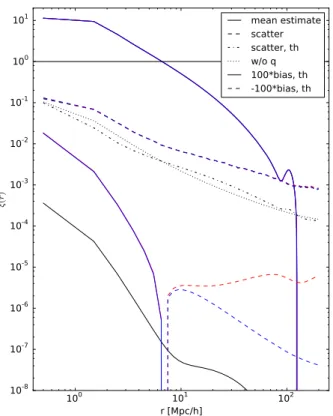
. 100 101 102 r [Mpc/h] 10-8 10-7 10-6 10-5 10-4 10-3 10-2 10-1 100 101 ξ( r) mean estimate scatter scatter, th w/o q 100*bias, th -100*bias, th
Fig. 1.Mean ξ(r) estimate and the scatter and theoretical bias of the estimates for different estimators. The dash-dotted line, our theoretical result for the scatter of the LS method, underestimates the scatter, since higher-order correlations in the D catalog are ignored. The dotted line is without the contribution of the q terms, and is dominated by the Poisson (p) terms. The bias is multiplied by 100 so the curves can be displayed in a more compact plot. For the measured mean and scatter, and the theoretical bias we plot standard LS in black, dilution with d= 0.14 in red, and split with Ms = 50 in blue. For the mean and scatter the
dif-ference between the methods is not visible in this plot. The difdif-ferences in the mean estimate are shown in Fig.5. The differences in scatter (or
its square, the variance) are shown in Fig3. For the theoretical bias the difference between split and dilution is not visible at small r (ξ(r) > 1), where the bias is positive.
3.2. Optimizing computational cost and variance of the split method
The bias is small compared to variance in our application (see Fig.1for the theoretical result and Fig.5for an attempted bias measurement), and therefore we focus on variance as the figure of merit. The computational cost should be roughly proportional to 1 2N 2 d 1+ 2Mr+ Mr2 Ms ! =: 1 2N 2 dc, (27)
and the additional variance due to finite R catalog in the ξ → 0 limit becomes ∆var ≈ 2 Mr + Ms M2 r ! p=: vp. (28)
Here, Nd and p are fixed by the survey and the requested r
bin-ning, but we can vary Mr and Ms in the search for the optimal
computational method. In the above we defined the “cost” and “variance” factors c and v.
We may ask two questions:
1. For a fixed level of variance v, which combination of Mrand
2. For a fixed computational cost c, which combination of Mr
and Msminimizes the variance v?
The answer to both questions is (Slepian & Eisenstein 2015) Ms= Mr ⇒ c= 1 + 3Mr and v =
3 Mr
· (29)
Thus, the optimal version of the split method is the natural one where N0
r = Nd. In this case the additional variance in the
ξ → 0 limit becomes ∆var ≈ 2Nd N0 r +Nd N0 r ! p, (30)
and the computational cost factor Nd2+ 2NdNr+ Nr0N 0 r becomes 1+ 2N 0 r Nd + Nr0 Nd ! N2d, (31)
meaning that DR pairs contribute twice as much as RR pairs to the variance and also twice as much computational cost is invested in them. The memory requirement for the random cata-log is then the same as for the data catacata-log. The cost saving esti-mate above is optimistic, since the computation involves some overhead not proportional to the number of pairs.
For small scales, where ξ 1, the situation is different. The greater density of DD pairs due to the correlation requires a greater density of the R catalog so that the additional variance from it is not greater. From Eq. (19) we see that the balance of the DR and the RR contributions is different for large ξ (the pc
term vs. the other terms). We may consider recomputing ˆξ for the small scales using a smaller rmaxand a larger R catalog.
Consid-ering just the Poisson terms (pcand pror p0r) with a
“representa-tive” ξ value, (27) and (28) become c= 1 + ξ + 2 Mr+ M2r/Ms
and v= 2/Mr+ (1 − ξ)2Ms/M2r which modifies the above result
(Eq. (29)) for the optimal choice of Msand Mrto
Ms=
Mr
|ξ − 1|, that is, Nr0= |ξ − 1|Nd. (32)
This result is only indicative, since it assumes a constant ξ for r< rmax. In particular, it does not apply for ξ ≈ 1, because then
the approximation of ignoring the qr and tr terms in (19) is not good.
4. Tests on mock catalogs
4.1. Minerva simulations and methodology
The Minerva mocks are a set of 300 cosmological mocks pro-duced with N-body simulations (Grieb et al. 2016;Lippich et al. 2019), stored at five output redshifts z ∈ {2.0, 1.0, 0.57, 0.3, 0}. The cosmology is flatΛCDM with Ωm= 0.285, and we use the
z = 1 outputs. The mocks have Nd ≈ 4 × 10⁶ objects (“halos”
found by a friends-of-friend algorithm) in a box of 1500 h−1Mpc
cubed.
To model the survey geometry of a redshift bin with∆z ≈ 0.1 at z ∼ 1, we placed the observer at comoving distance 2284.63 h−1Mpc from the center of the cube and selected from
the cube a shell 2201.34–2367.92 h−1Mpc from the observer. The comoving thickness of the shell is 166.58 h−1Mpc. The
resulting mock sub-catalogs have Nd ≈ 4.5 × 10⁵ and are
rep-resentative of the galaxy number density of the future Euclid spectroscopic galaxy catalog.
We ignore peculiar velocities, that is, we perform our anal-ysis in real space. Therefore, we consider results for the 1D
2PCF ξ(r). We estimated ξ(r) up to rmax = 200 h−1Mpc using
∆r = 1 h−1Mpc bins.
We chose standard LS with Mr= 50 as the reference method.
In the following, LS without further qualification refers to this. The random catalog was generated separately for each shell mock to measure their contribution to the variance. For one of the random catalogs we calculated also triplets to obtain the edge effect quantity Ndt12= Gt12/G
p 1G
p 2− 1.
While dilution can already be discarded on theoretical grounds, we show results obtained using dilution, since these results provide the scale for edge effects demonstrating the importance of eliminating them with a careful choice of method. For the dilution and split methods we also used Mr = 50, and
tried out dilution fractions d := N0
r/Nr0= 0.5, 0.25, 0.14 and split
factors Ms = 4, 16, 50 (chosen to have similar pairwise
com-putational costs). In addition, we considered standard LS with Mr = 25, which has the same number of RR pairs as d = 0.5 and
Ms = 4, but only half the number of DR pairs; and standard LS
with Mr = 1 to demonstrate the effect of a small Nr0.
The code used to estimate the 2PCF implements a highly optimized pair-counting method, specifically designed for the search of object pairs in a given range of separations. In par-ticular, the code provides two alternative counting methods, the chain-mesh and the kd-tree. Both methods measure the exact number of object pairs in separation bins, without any approx-imation. However, since they implement different algorithms to search for pairs, they perform differently at different scales, both in terms of CPU time and memory usage. Overall, the efficiency of the two methods depends on the ratio between the scale range of the searching region and the maximum separation between the objects in the catalog.
The kd-tree method first constructs a space-partitioning data structure that is filled with catalog objects. The minimum and maximum separations probed by the objects are kept in the data structure and are used to prune object pairs with separations outside the range of interest. The tree pair search is performed through the dual-tree method in which cross-pairs between two dual trees are explored. This is an improvement in terms of exploration time over the single-tree method.
On the other hand, in the chain-mesh method the catalog is divided in cubic cells of equal size, and the indexes of the objects in each cell are stored in vectors. To avoid counting object pairs with separations outside the interest range, the counting is performed only on the cells in a selected range of distances from each object. The chain-mesh algorithm has been imported from the CosmoBolognaLib, a large set of free software C++/ python libraries for cosmological calculations (Marulli et al. 2016).
For our test runs we used the chain-mesh method. 4.2. Variance and bias
In Fig.1we show the mean (over the 300 mock shells) estimated correlation function and the scatter (square root of the variance) of the estimates using the LS, split, and dilution methods; our theoretical approximate result for the scatter for LS; and our the-oretical result for bias for the different methods.
The theoretical result for the scatter is shown with and with-out the q terms, which include the triplet correlation ξ12, for
which we used here the approximation ξ12≈ξ(max(r1, r2)). This
behaves as expected, that is, it underestimates the variance, since we neglected the higher-order correlations in the D catalog. Nev-ertheless, it (see the dash-dotted line in Fig.1) has similar fea-tures to the measured variance (dashed lines).
100 101 102 r [Mpc/h] 10-12 10-11 10-10 10-9 10-8 10-7 10-6 10-5 10-4 10-3 10-2 p pc pr q qr t tr
Fig. 2.Quantities p, pc, pr, q, qr, t, and tr for the Minerva shell. The
values for the first bin are noisy. The vertical red line marks r= L.
0 50 100 150 200 r [Mpc/h] −0.5 0.0 0.5 1.0 1.5 2.0 2.5 r 2va r [ξ (r )] di ffe ren ce fr om LS 1e−3 LS, Nr = Nd dilu ion = 0.14 dilu ion = 0.25 dilu ion = 0.5 LS, Nr = 25Nd spli = 50 spli = 16 spli = 4
Fig. 3.Measured difference from LS of the variance of different
estima-tors, multiplied by r2. Dashed lines are our theoretical results.
In Fig.2we plot the diagonals of the p, t, and q quantities. This shows how their relative importance changes with separa-tion scale. It also confirms that our initial assumpsepara-tion on small relative fluctuations is valid in this simulation case.
Consider now the variance differences (from standard LS with Mr= 50), for which our theoretical results should be
accu-rate. Figure3compares the measured variance difference to the theoretical result. For the diluted estimators and LS with Mr = 1
the measured result agrees with theory, although clearly the mea-surement with just 300 mocks is rather noisy. For the split esti-mators and LS with Mr = 25 the difference is too small to be
appreciated with 300 mocks, but at least the measurement does not disagree with the theoretical result.
In Fig. 4we show the relative theoretical increase in scat-ter compared to the best possible case, which is LS in the limit Mr → ∞. Since we do not have a valid theoretical result for the
total scatter, we estimate it by subtracting the theoretical di ffer-ence from LS with Mr = 50 from the measured variance of the
latter.
At scales r . 10 h−1Mpc the theoretical prediction is about the same for dilution and split and neither method looks promis-ing for r 10 h−1Mpc where ξ 1. This suggests that for optimizing cost and accuracy, a different method should be used
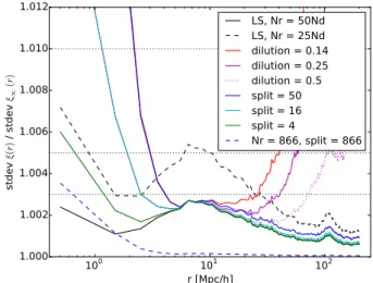
100 101 102 r [Mpc/h] 1.000 1.002 1.004 1.006 1.008 1.010 1.012 st de v ξ( r) / st de v ξ∞ (r ) LS, Nr = 50Nd LS, Nr = 25Nd dilution = 0.14 dilution = 0.25 dilution = 0.5 split = 50 split = 16 split = 4 Nr = 866, split = 866
Fig. 4.Theoretical estimate of the scatter of the ξ estimates divided by the scatter in the N0
r → ∞ limit. The dotted lines correspond to 0.3%,
0.5%, and 1% increase in scatter. For r < 10 h−1Mpc there is hardly
any difference between split and dilution, the curves lie on top of each other; whereas for larger r split is much better.
0 50 100 150 200 r [Mpc/h] −0.006 −0.004 −0.002 0.000 0.002 0.004 0.006 0.008 r( ξ( r) − ξLS (r )) LS, Nr = Nd LS, Nr = 25Nd dilution = 0.5 dilution = 0.25 dilution = 0.14 split = 4 split = 16 split = 50
Fig. 5.Differences between the mean ξ(r) estimate and that from the LS, multiplied by r to better display all scales. This measured difference is not the true bias, which is too small to measure with 300 mocks, and is mainly due to random error of the mean. The results for dilution appear to reveal a systematic bias, but this is just due to strong error correlations between nearby bins; for different subsets of the 300 mocks the mean difference is completely different.
for smaller scales than that used for large scales. The number of RR pairs with small separations is much less. Therefore, for the small-scale computation there is no need to restrict the com-putation to a subset of RR pairs, or alternatively, one can afford to increase Mr. For the small scales, we may consider the split
method with increased Mras an alternative to standard LS. We
have the same number of pairs to compute as in the reference LS case, if we use Mr = 866 and Ms = 866. We added this case to
Fig.4. It seems to perform better than LS at intermediate scales, but for the smallest scales LS has the smaller variance. This is in line with our conclusion in Sect.3.2, which is that when ξ 1, it is not optimal to split the R catalog into small subsets.
We also compared the differences in the mean estimate from the different estimators to our theoretical results on the bias differences (see Fig.5), but the theoretical bias differences are much smaller than the expected error of the mean from
Table 1. Mean computation time over the 300 runs and the mean vari-ance over four different ranges of r bins (given in units of h−1Mpc) for
each method.
Method Time Mean variance
[s] 0–2 5–15 80–120 150–200 [×10−2] [×10−5] [×10−6] [×10−7] Mr = 50 7889 1.01 4.42 1.23 7.01 Mr = 25 2306 1.01 4.39 1.23 7.04 Mr = 1 16.5 5.96 5.53 1.46 8.05 d= 0.5 2239 1.01 4.41 1.25 7.11 d= 0.25 812 1.02 4.41 1.25 7.42 d= 0.14 487 1.08 4.41 1.28 7.72 Ms= 4 1854 1.01 4.42 1.23 7.02 Ms= 16 763 1.00 4.42 1.23 7.01 Ms= 50 593 1.09 4.42 1.23 7.02
Notes. The first three are standard LS. The variance cannot be measured accurately enough from 300 realizations to correctly show all the di ffer-ences between methods. Thus the table shows some apparent improve-ments (going from Mr= 50 to Mr= 25 and from Ms= 4 to Ms = 16),
which are not to be taken as real. See Fig.6for the fifth vs. second column with error bars.
300 mocks; and we simply confirm that the differences we see are consistent with the error of the mean and thus consistent with the true bias being much smaller. We also performed tests with completely random (ξ = 0) mocks, and with a large number (10 000) of mocks confirmed the theoretical bias result for the different estimators in this case. Since the bias is too small to be interesting we do not report these results in more detail here.
However, we note that for the estimation of the 2D 2PCF and its multipoles, the 2D bins will contain a smaller number of objects than the 1D bins of these test runs and therefore the bias is larger. Using the theoretical results (17) or (24) the bias can be removed afterwards with accuracy depending on how well we know the true ξ.
4.3. Computation time and variance
The test runs were made using a single full 24-core node for each run. Table1shows the mean computation time and mean estimator variance for different r ranges for the different cases we tested. Of these r ranges, the r= 80−120 h−1Mpc is perhaps
the most interesting, since it contains the important BAO scale. Therefore, we plot the mean variance at this range versus mean computation time in Fig.6, together with our theoretical predic-tions. The theoretical estimate for the computation time for other dilution fractions and split factors is
(1+ 24.75d2) 306 s and (1+ 24.75/Ms2) 306 s, (33) assuming Mr = 50. For standard LS with other random catalog
sizes, the computation time estimate is
(1+ 2 Mr+ M2r) 3.03 s. (34)
5. Conclusions
The computational time of the standard Landy–Szalay estimator is dominated by the RR pairs. However, except at small scales where correlations are large, these make a negligible contribu-tion to the expected error compared to the contribucontribu-tion from the
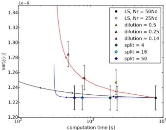
102 103 104 computation time [s] 1.20 1.22 1.24 1.26 1.28 1.30 1.32 1.34 va r [ξ (r )] 1e 6 LS, Nr = 50Nd LS, Nr = 25Nd dilution = 0.5 dilution = 0.25 dilution = 0.14 split = 4 split = 16 split = 50
Fig. 6. Measured variance (mean variance over the range r = 80−120 h−1Mpc) vs. computational cost (mean computation time) for
the different methods (markers with error bars) and our theoretical pre-diction (solid lines). The solid lines (blue for the split method, red for dilution, and black for standard LS with Mr ≤ 50) are our theoretical
predictions for the increase in variance and computation time ratio when compared to the standard LS, Mr= 50, case, and the dots on the curves
correspond to the measured cases (except for LS they are, from right to left, Mr= 25, 12.5, and (50/7); only the first of which was measured).
The curve for split ends at Ms= 2500; the optimal case, Ms= Mr, is the
circled dot. The error bars for the variance measurement are naive esti-mates that do not account for error correlations between bins. The the-oretical predictions overestimate the cost savings (data points are to the right of the dots on curves; except for the smaller split factors, where the additional speed-up compared to theory is related to some other perfor-mance differences between our split and standard LS implementations). This plot would have a different appearance for other r ranges.
DDand DR pairs. Therefore, a substantial saving of computa-tion time with an insignificant loss of accuracy can be achieved by counting a smaller subset of RR pairs.
We considered two ways to reduce the number of RR pairs: dilution and split. In dilution, only a subset of the R catalog is used for RR pairs. In split, the R catalog is split into a number of smaller subcatalogs, and only pairs within each subcatalog are counted. We derived theoretical results for the additional esti-mator covariance and bias due to the finite size of the random catalog for these different variants of the LS estimator, extend-ing in many ways the original results byLandy & Szalay(1993), who worked in the limit of an infinite random catalog. We tested our results using 300 mock data catalogs, representative of the z = 0.95–1.05 redshift range of the future Euclid survey. The split method maintains the property the Landy–Szalay estimator was designed for, namely cancelation of edge effects in bias and variance (for ξ= 0), whereas dilution loses this cancellation and therefore should not be used.
For small scales, where correlations are large, one should not reduce RR counts as much. The natural dividing line is the scale r where ξ(r) = 1. Interestingly, the difference in bias and covariance between the different estimators (split, dilution, and LS) vanishes when ξ= 1. We recommend the natural version of the split method, Ms = Mr, for large scales where |ξ| < 1. This
leads to a saving in computation time by more than a factor of ten (assuming Mr = 50) with a negligible effect on variance and bias.
For small scales, where ξ > 1, one should consider using a larger random catalog and one can use either the standard LS method or the split method with a more modest split factor. Because the
number of pairs with these small separations is much smaller, the computation time is not a similar issue as for large separations.
The results of our analysis will have an impact also on the computationally more demanding task of covariance matrix esti-mation. However, since in that case the exact computational cost is determined by the balance of data catalogs and random cata-logs, which does not need to be the same as for the individual two-point correlation estimate, we postpone a quantitative anal-ysis to a future, dedicated study. The same kind of methods can be applied to higher-order statistics (three-point and four-point correlation functions) to speed up their estimation (Slepian & Eisenstein 2015).
Acknowledgements. We thank Will Percival and Cristiano Porciani for use-ful discussions. The 2PCF computations were done at the Euclid Science Data Center Finland (SDC-FI, urn:nbn:fi:research-infras-2016072529), for whose computational resources we thank CSC – IT Center for Science, the Finnish Grid and Cloud Computing Infrastructure (FGCI, urn:nbn:fi:research-infras-2016072533), and the Academy of Finland grant 292882. This work was sup-ported by the Academy of Finland grant 295113. VL was supsup-ported by the Jenny and Antti Wihuri Foundation, AV by the Väisälä Foundation, AS by the Mag-nus Ehrnrooth Foundation, and JV by the Finnish Cultural Foundation. We also acknowledge travel support from the Jenny and Antti Wihuri Foundation. VA acknowledges funding from the European Union’s Horizon 2020 research and innovation programme under grant agreement No 749348. FM acknowledges the grants ASI n.I/023/12/0 “Attivit‘a relative alla fase B2/C per la missione Euclid” and PRIN MIUR 2015 “Cosmology and Fundamental Physics: illuminating the Dark Universe with Euclid”.
References
Alam, S., Ata, M., Bailey, S., et al. 2017,MNRAS, 470, 2617
Alcock, C., & Paczy´nski, B. 1979,Nature, 281, 358
Alonso, D. 2012, ArXiv e-prints [arXiv:1210.1833]
Anderson, L., Aubourg, E., Bailey, S., et al. 2012,MNRAS, 427, 3435
Anderson, L., Aubourg, E., Bailey, S., et al. 2014,MNRAS, 441, 24
Ata, M., Baumgarten, F., Bautista, J., et al. 2018,MNRAS, 473, 4773
Bautista, J. E., Vargas-Magaña, M., Dawson, K. S., et al. 2018,ApJ, 863, 110
Bernstein, G. M. 1994,ApJ, 424, 569
Beutler, F., Blake, C., Colless, M., et al. 2011,MNRAS, 416, 3017
Beutler, F., Blake, C., Colless, M., et al. 2012,MNRAS, 423, 3430
Blake, C., Kazin, E. A., Beutler, F., et al. 2011,MNRAS, 418, 1707
Cole, S., Percival, W. J., Peacock, J. A., et al. 2005,MNRAS, 362, 505
Davis, M., & Peebles, P. J. E. 1983,ApJ, 267, 465
de la Torre, S., Jullo, E., Giocoli, C., et al. 2017,A&A, 608, A44
Demina, R., Cheong, S., BenZvi, S., & Hindrichs, O. 2018,MNRAS, 480, 49
Eisenstein, D. J., Zehavi, I., Hogg, D. W., et al. 2005,ApJ, 633, 560
Grieb, J. N., Sánchez, A. G., Salvador-Albornoz, S., & Dalla Vecchia, C. 2016,
MNRAS, 457, 1577
Guzzo, L., Pierleoni, M., Meneux, B., et al. 2008,Nature, 451, 541
Hamilton, A. J. S. 1993,ApJ, 417, 19
Hewett, H. C. 1982,MNRAS, 201, 867
Hou, J., Sánchez, A. G., Scoccimarro, R., et al. 2018,MNRAS, 480, 2521
Jarvis, M. 2015, Astrophysics Source Code Library [record ascl:1508.007] Kaiser, N. 1987,MNRAS, 227, 1
Kerscher, M. 1999,A&A, 343, 333
Kerscher, M., Szapudi, I., & Szalay, A. S. 2000,ApJ, 535, L13
Landy, S. D., & Szalay, A. S. 1993,ApJ, 412, 64
Laureijs, R., Amiaux, J., Arduini, S., et al. 2011, ArXiv e-prints [arXiv:1110.3193]
Lippich, M., Sánchez, A. G., Colavincenzo, M., et al. 2019,MNRAS, 482, 1786
Marulli, F., Veropalumbo, A., & Moresco, M. 2016,Astron. Comput., 14, 35
Moore, A., Connolly, A., Genovese, C., et al. 2000, ArXiv e-prints [arXiv:astro-ph/0012333]
Peacock, J. A., Cole, S., Norberg, P., et al. 2001,Nature, 410, 169
Peebles, P. J. E., & Hauser, M. G. 1974,ApJS, 28, 19
Percival, W. J., Reid, B. A., Eisenstein, D. J., et al. 2010,MNRAS, 401, 2148
Pezzotta, A., de la Torre, S., Bel, J., et al. 2017,A&A, 604, A33
Reid, B. A., Samushia, L., White, M., et al. 2012,MNRAS, 426, 2719
Ross, A. J., Samushia, L., Howlett, C., et al. 2015,MNRAS, 449, 835
Ross, A. J., Beutler, F., Chuang, C. H., et al. 2017,MNRAS, 464, 1168
Ruggeri, R., Percival, W. J., Gil-Marín, H., et al. 2019,MNRAS, 483, 3878
Slepian, Z., & Eisenstein, D. J. 2015,MNRAS, 454, 4142
Vargas-Magaña, M., Ho, S., Cuesta, A. J., et al. 2018,MNRAS, 477, 1153
Wall, J. V., & Jenkins, C. R. 2012, Practical Statistics for Astronomers
(Cambridge, UK: Cambridge University Press)
Zarrouk, P., Burtin, E., Gil-Marín, H., et al. 2018,MNRAS, 477, 1639
Appendix A: Derivation examples
As examples of how the variances of the different deviations, hαβi and so on, are derived, following the method presented in LS93, we give three of the cases here: hα1α2i (common for all
the variants of LS), and hβ1γ02i and hγ01γ02i for the split method.
The rest are calculated in a similar manner.
To derive the hDD1DD2i appearing in the hα1α2i of (15) we
start from hDD1DD2i= K X i< j K X k<l hninjnknliΘi j(r1)Θkl(r2), (A.1)
where both i, j, and k, l sum over all microcell pairs; ni = 1 or 0
is the number of galaxies in microcell i. There are three different cases for the terms hninjnknli depending on how many indices
are equal (i , j and k , l for all of them).
The first case (quadruplets, i.e., two pairs of microcells) is when i, j, k, l are all different. We use P∗i jklto denote this part of the sum. There are12K(K − 1) ×12(K − 2)(K − 3)=14K4(we work in the limit K → ∞) such terms and they have
hninjnknli = Nd K Nd− 1 K −1 Nd− 2 K −2 Nd− 3 K −3 D (1+ δi)(1+ δj)(1+ δk)(1+ δl) E = Nd(Nd− 1)(Nd− 2)(Nd− 3) K4 h 1+ hδiδji+ hδkδli+ hδiδki + hδiδli+ hδjδki+ hδjδli + hδiδjδki+ hδiδjδli+ hδiδkδli+ hδjδkδli+ hδiδjδkδli i = Nd(Nd− 1)(Nd− 2)(Nd− 3) K4 h 1+ ξ(ri j)+ ξ(rkl)+ ξ(rik) + ξ(ril)+ ξ(rjk)+ ξ(rjl) + ζ(xi, xj, xk)+ ζ(xi, xk, xl)+ ζ(xi, xj, xl)+ ζ(xj, xk, xl) + ξ(ri j)ξ(rkl)+ ξ(rik)ξ(rjl)+ ξ(ril)ξ(rjk) + η(xi, xj, xk, xl)i, (A.2)
where δi := δ(xi) is the density perturbation (relative to the
actual mean density of galaxies in the survey), ζ is the three-point correlation, and η is the connected (i.e., the part that does not arise from the two-point correlation) four-point correlation. The fraction of microcell quadruplets (pairs of pairs) that satisfy ri j ≡xj−xi ∈ r1and rkl ∈r2 is Gp(r1)Gp(r2)=: G
p 1G
p 2. In the
limit of large K the number of other index quadruplets is negli-gible compared to those where all indices have different values, so we have ∗ X i jkl Θi j 1Θ kl 2 = K(K − 1)(K − 2)(K − 3) 4 G p 1G p 2= K4 4 G p 1G p 2. (A.3)
For the connected pairs (i, j) and (k, l) we have ξ(ri j)= ξ(r1) ≡
ξ1and ξ(rkl)= ξ(r2) ≡ ξ2.
The second case (triplets of microcells) is when k or l is equal to i or j. We denote this part of the sum by
∗ X i jk hninjnkiΘik1Θ jk 2. (A.4)
It turns out that it goes over all ordered combinations of {i, j, k}, where i, j, k are all different, exactly once, so there are
K(K − 1)(K − 2)= K3such terms (triplets). Here
hninjnki= Nd K Nd− 1 K −1 Nd− 2 K −2 D (1+ δi)(1+ δj)(1+ δk) E = Nd(Nd− 1)(Nd− 2) K3 h 1+ hδiδki+ hδjδki+ hδiδji+ hδiδjδki i = Nd(Nd− 1)(Nd− 2) K3 h 1+ ξ(rik)+ ξ(rjk)+ ξ(ri j)+ ζ(xi, xj, xk)i, (A.5) and ∗ X i jk Θik 1Θ jk 2 = K 3 Gt12. (A.6)
The third case (pairs of microcells) is when i= k and j = l. This part of the sum becomes
X i< j hninjiΘ i j 1Θ i j 2, (A.7) where hninji= Nd(Nd− 1) K2 h 1+ ξ(ri j)i , (A.8) and X i< j Θi j 1Θ i j 2 = δ12 K2 2 G p 1, (A.9)
that is, the sum vanishes unless the two bins are the same, r1 =
r2.
We now apply the three approximations listed in Sect. 2.2: (1) ξ(rik) = ξ(ril) = ξ(rjk) = ξ(rjl) = 0 in (A.2); (2) ζ = 0 in
(A.2) and (A.5); (3) η= 0 in (A.2). We obtain hDD1DD2i ' 1 4Nd(Nd− 1)(Nd− 2)(Nd− 3)(1+ ξ1)(1+ ξ2)G p 1G p 2 + Nd(Nd− 1)(Nd− 2)(1+ ξ1+ ξ2+ ξ12)Gt12 +1 2Nd(Nd− 1)δ12(1+ ξ1)G p 1, (A.10)
and using hDDi from (3) we arrive at the hα1α2i result given in
Eq. (15).
For the split method, we give the calculation for hγ0 1β 0 2i= hRR0 1DR2i − hRR 0 1ihDR2i hRR0 1ihDR2i , hγ0 1γ 0 2i= hRR0 1RR 0 2i − hRR 0 1ihRR 0 2i hRR0 1ihRR 0 2i (A.11) below. First the hγ01β2i: hRR01DR2i= Ms X µ=1 hRµRµ1DR2i= MshRµR µ 1 DR2i, (A.12) where hRµRµ1DR2i= X i< j X k,l hsisjnkrliΘ i j 1Θ kl 2, (A.13)
siis the number (0 or 1) of Rµobjects in microcell i, and rlis the
There are 12K4 quadruplet terms, for which (see (A.3)) P∗ΘΘ = 1 2K 4Gp 1G p 2, and hsisjnkrli= N0r(Nr0− 1)Nd(Nr0− 2) K4 · (A.14)
Triplets where i or j is equal to k have hsisknkrli = 0, since
sknk= 0 always (we cannot have two objects, from Rµand D, in
the same cell). There are K3triplet terms where i or j is equal to
l: for themP∗ΘΘ = K3Gt 12, and hsislnkrli= hsislnki= N0 r(Nr0− 1)Nd K3 , (A.15)
where if sl= 1 then also rl= 1 since Rµ⊂ R.
Pairs where (i, j)= (k, l) or (i, j) = (l, k) have hskslnkrli= 0,
since again we cannot have two different objects in the same cell. Thus hRR0 1DR2i= 1 2NdNr(N 0 r− 1)(N 0 r− 2)G p 1G p 2+ NdNr(N 0 r− 1)G t 12, (A.16)
and we obtain that hγ0 1β2i= 2 N0 r Gt 12 Gp1Gp2 − 1 = 2 t r 12, (A.17)
which is equal to the hγ1β2i of standard LS.
Then the hγ0 1γ 0 2i: hRR01RR02i= Ms X µ=1 Ms X ν=1 hRµRµ1· RνRν2i, (A.18)
where there are Ms(Ms− 1) terms with µ , ν giving
hRµRµ1RνRν2i= hRµRµ1ihRνRν2i=1 4(N 0 r)2(Nr0− 1)2G p 1G p 2, (A.19) and Msterms with µ= ν giving
hRµRµ1RµRµ2i=1 4N 0 r(N 0 r − 1)(N 0 r − 2)(N 0 r− 3)G p 1G p 2 + N0 r(N 0 r − 1)(N 0 r− 2)G t 12 +1 2N 0 r(N 0 r − 1)δ12G p 1. (A.20)
Adding these up gives hRR01RR02i= 1 4N 0 r(N 0 r− 1)(N 0 rN 0 r− N 0 r − 4 N 0 r + 6)G p 1G p 2 + N0 r(N 0 r − 1)(N 0 r − 2)G t 12 +1 2N 0 r(N 0 r − 1)δ12Gp1 (A.21) and hγ0 1γ 0 2i= 2 Nr0(Nr0− 1) 2(Nr0− 2) Gt12 Gp1Gp2 − 1 + δ12 Gp1 − 1 = 4 tr 12+ p r0 12. (A.22)
This differs both from standard LS and from dilution, since it involves both N0