HAL Id: hal-02271580
https://hal.inria.fr/hal-02271580
Submitted on 15 Nov 2019
HAL is a multi-disciplinary open access
archive for the deposit and dissemination of
sci-entific research documents, whether they are
pub-lished or not. The documents may come from
teaching and research institutions in France or
abroad, or from public or private research centers.
L’archive ouverte pluridisciplinaire HAL, est
destinée au dépôt et à la diffusion de documents
scientifiques de niveau recherche, publiés ou non,
émanant des établissements d’enseignement et de
recherche français ou étrangers, des laboratoires
publics ou privés.
Robust pedestrian trajectory reconstruction from
inertial sensor
Bertrand Beaufils, Frédéric Chazal, Marc Grelet, Bertrand Michel
To cite this version:
Bertrand Beaufils, Frédéric Chazal, Marc Grelet, Bertrand Michel. Robust pedestrian trajectory
reconstruction from inertial sensor. IPIN 2019 - 10th International Conference on Indoor Positioning
and Indoor Navigation, Sep 2019, Pisa, Italy. �hal-02271580�
Robust pedestrian trajectory reconstruction from
inertial sensor
Bertrand Beaufils
∗, Frédéric Chazal
†, Marc Grelet
‡and Bertrand Michel
§∗‡ Sysnav, 57 Rue de Montigny, 27200 Vernon, France
∗†§ Inria Saclay team DataShape, 1 Rue Honoré d’Estienne d’Orves, 91120 Palaiseau, France §Centrale Nantes Informatic and Mathematics Department, 1 Rue de La Noe, 44300 Nantes, France
Email:∗[email protected],†[email protected],‡[email protected],§[email protected]
Abstract—In this paper, a strides detection algorithm combined with a technique inspired by Zero Velocity Update (ZUPT) is proposed using inertial sensors worn on the ankle. This innovative approach based on a sensors alignment and machine learning can detect both normal walking strides and atypical strides such as small steps, side steps and backward walking that existing methods struggle to detect. As a consequence, the trajectory reconstruction achieves better performances in daily life contexts for example, where a lot of these kinds of strides are performed in narrow areas such as in a house. It is also robust in critical situations, when for example the wearer is sitting and moving the ankle or bicycling, while most algorithms in the literature would wrongly detect strides and produce error in the trajectory reconstruction by generating movements.
Our algorithm is evaluated on more than 7800 strides from seven different subjects performing several activities. We validated the trajectory reconstruction during motion capture sessions by analyzing the stride length. Finally, we tested the algorithm in a challenging situation by plotting the computed trajectory on the building map of an 5 hours and 30 minutes office worker recording.
I. INTRODUCTION
The emergence of Global Navigation Satellite System (GNSS) receivers in the 2000s has changed the perception of navigation. While they are commonly used in outdoor envi-ronments they fail to produce accurate localization due to poor reception in many situations, for example in tunnels, indoor parking, in the forest, inside buildings etc. Instead, body-mounted inertial measurement units (IMUs) can be used to record the movements of pedestrians, providing an estimate of their motion relative to a known origin. Unlike infrastructure-dependent localization systems such as map matching, Wi-Fi [1], Radio Frequency Identification [2] or ultra-wideband [3], body-mounted IMUs are lightweight and can be rapidly and easily deployed.
In this context, Sysnav has developed WATA systems (Wear-able Ankle Trajectory Analyzer) based on magneto-inertial sensors [4], [5], to enable trajectory reconstruction. Here we consider an ankle worn device for dead reckoning. The strategy which consists in the integration of the linear acceleration and angular velocity data from the unit may rapidly cumulate large errors due to IMUs drifts. To overcome this issue, we use
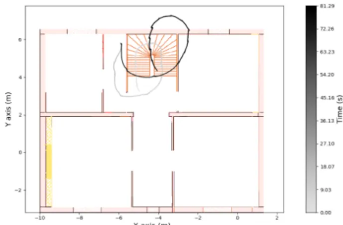
a technique inspired by Zero Velocity Update (ZUPT) [6]– [9], which is an effective method to limit the accumulation of errors. It consists in correcting the speed drift by estimating the speed of the ankle when the foot is on the ground during the walk and then integrates the data only between two ZUPTs. Several studies [10], [11], propose to detect pedestrian movements and classify activities (such as walking, stairs climbing, running...) from inertial data. These approaches do not work well outside a controlled environment [12]. Moreover these methods based on sliding windows do not allow to detect individual strides. A few methods of stance detection have been proposed in the literature by tuning thresholds to determine the start and the end of the strides [13]–[15]. Sysnav first developed a similar approach based on the swing detection and a combination of criteria on the inertial data to determine the ZUPT instant (accelerations close to one g and small values of the angular velocity). These methods show good results for classical gait but they tend to fail for atypical strides such as stairs and small steps. In order to give an illustration of these limits, we ask a wearer to climb the stairs and get in a small corridor where he performs small steps before going back. We plot in Figure 1 the computed trajectory by the Sysnav algorithm. It illustrates that during the atypical strides in the
Fig. 1: Computed trajectory with a strides detection based on inertial thresholds.
corridor, no stride is detected as the trajectory stays on the same point for dozens of seconds. In the end, the error is about two meters.
Other approaches use machine learning techniques on the frequency characteristics of the signals [16], [17]. These meth-ods show good results when it is known that the pedestrian is walking but fail in a lot of real life situations. Indeed, several foot movements in sitting position and bicycling for example are wrongly detected as strides.
In this work we describe our step detector which is based on a innovative technique to compute a sensors alignment for inertial data that enables a extraction of intervals that may correspond to strides. The selection among them is performed by a classifier built with the Gradient Boosting Tree algorithm. The same approach can also be applied to recognize the activity of the performed step. Activity recognition can be a valuable information in many situations, for example in med-ical context, but we focus here on trajectory reconstruction.
II. TERRESTRIAL REFERENCE FRAME COMPUTATION
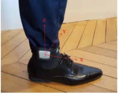
The system should be worn at the ankle as illustrated in Figure 2. In this default placement, the sensors record the inertial data in the reference frame defined by the Z axis aligned with the leg and the X axis aligned with the foot. However we observed that the device may be worn upside down and may turn around the ankle during the recording. The machine learning approach in this algorithm requires the 3-D inertial data to be in the same reference frame definition. In a previous work [18] we described a method that aligns the sensors based on geometric patterns of the angular velocity data. In this paper we present a more robust technique that has the particularity of removing the gravity from the acceleration data and compute a terrestrial reference frame. Indeed, the accelerometer in the device records the linear acceleration (Γ) that is equal to the gravity added to the acceleration of the WATA system (ΓAnkle).
Fig. 2: Default device placement.
The main idea lies in the fact that in an inertial reference frame, the integration of ΓAnkle is equal to the difference of the ankle speed (a few meters per second for a pedestrian) that is small compared to the integration of the gravity. At any time t in [0, tf inal], the device records the acceleration and angular
velocity data (respectively ΓBt(t) and ΩBt(t) in R
3) in the
body reference frame of the system Bt. With a no integration
error of the angular velocity, Rt solution of Equation 1 the
following would be the rotation matrix between Bt and B0.
dRt
dt = −Rt Skew(ΩBt(t)), (1)
with R0= I3 and the Skew operator defined for all vector n
inR3, n = (nx, ny, nz)T : Skew(n) = 0 −nz ny nz 0 −nx −ny nx 0 .
In practice, due to gyrometer imperfections (bias, non linear-ities, noise...), the product of the computed rotation matrix Rt and Bt only approximates B0. We note ˆB0t the resulting
reference frame. We can now express for all t the inertial data in the reference frame ˆBt
0 as follows: (Γ ˆ Bt 0(t) = RtΓBt(t), ΩBˆt 0(t) = RtΩBt(t). (2)
Let ΓAnkleBt (t) be the acceleration of the WATA system without the gravity gBt: ΓBt(t) = Γ
Ankle
Bt (t) + gBt. Then the mean of
the recorded acceleration projected in ˆBt
0, on an interval ∆T , is given by: 1 ∆T Zt+∆T t ΓBˆu 0(u)du = 1 ∆T Zt+∆T t (ΓAnkleBˆu 0 (u) + gBˆu 0)du.
We assume that for a ∆T small enough, the reference frame ˆ
B0uis constant for all u in [t, t + ∆T ]: ∀u ∈ [t, t + ∆T ], ˆBu0 =
ˆ Bt
0. Namely, we consider that during a small period, the
integration of the angular velocity produces no error. As a result, gBˆu
0 is a constant gBˆt0 on this interval, we have:
1 ∆T Zt+∆T t ΓBˆu 0(u)du = 1 ∆T Zt+∆T t ΓBˆt 0(u)du = 1 ∆T Zt+∆T t (ΓAnkleˆ Bt 0 (u) + gBˆt 0)du = 1 ∆T Zt+∆T t ΓAnkle ˆ Bt 0 (u)du + gBˆt 0. Let VBAnkleˆt 0
(u) be the speed of the ankle in the reference frame ˆ
B0t for all u in [t, t + ∆T ]. From the equation above we can write: 1 ∆T Z t+∆T t ΓBˆt 0(u)du = VAnkle ˆ Bt 0 (t + ∆T ) − VAnkle ˆ Bt 0 (t) ∆T + gB0.
For a sufficiently long duration of integration ∆T , we assume that the speed difference of the ankle, between t + ∆T and t, divided by ∆T is small compared to the gravity:
VAnkle ˆ Bt 0 (t + ∆T ) − VAnkle ˆ Bt 0 (t) ∆T gBˆt0. (3)
Thus, we can deduce the following equation:
1 ∆T Z t+∆T t ΓBˆu 0(u)du ≈ gBˆ0t. (4)
The assumption in Equation 3 is valid for large ∆T value. However, this approach requires to compute the mean of the acceleration in an inertial reference frame. Due to the integration drift with time, if ∆T is too large we have no guarantee that ˆBu
0 equals ˆB0tfor all u in [t + ∆T ]. In practice,
we found a compromise by setting ∆T = 15s.
Thanks to Equation 4 we can identify the gravity in the body reference frame at t = 0: gBˆ0
0 = gB0. If the angular velocity
integration did not produce any error, for all t > 0 gBˆt 0 would
be equals to gB0. In practice we observe that gBˆt
0 changes
all t > 0 we can correct it by computing the rotation matrix Rgt that aligns gBˆt
0 over time. We introduce the vector a as
follows: a = lim dt→0 gBˆt 0/||gBˆt0 || × gˆ B0t+dt/||gBˆ0t+dt|| dt .
Then the rotation matrix Rgt is the solution of the following
equation:
dRgt
dt = −R
g
t Skew(a) (5)
Then we can project the inertial data in the initial body reference frame for all t > 0:
(Γ B0(t) = R g t ΓBˆt 0(t) = R g t RtΓBt(t), ΩB0(t) = R g t ΩBˆt 0(t) = R g t RtΩBt(t). (6)
We now define a terrestrial reference frame Bterr by
consid-ering the vector − gB0
||gB0|| as the new Z
terraxis and choosing
arbitrarily Xterrand Yterraxes in order to build an
orthonor-mal basis. We note Rterr the rotation matrix between Bterr
and B0. The inertial data projected in the terrestrial reference
frame are given by the following for all t:
(
ΓBterr(t) = RterrΓB0(t),
ΩBterr(t) = RterrΩB0(t).
(7)
We have now access to the acceleration of the ankle for all t by removing the gravity (≈ 9, 81m/s) from the Zterr axis:
ΓAnkleBterr(t) = ΓBterr(t) −
0 0 9, 81 . (8)
The advantage of the attitude filter is the efficiency of its computation. This characteristic is necessary as we use ΓAnkleBterr to compute a pseudo-speed that is one of the main
features in our step detector. Indeed, due to the complexity of our application framework, it is difficult to describe a stride detector with only inertial models. In Section III, the computation of a pseudo-speed is introduced. It allows to extract a family of candidate intervals that may correspond to strides.
III. PSEUDO-SPEED COMPUTATION
A. Integration of the ankle acceleration
In previous Section II, we described the projection of the inertial data recorded by the device into a terrestrial reference frame Bterr. In this procedure, the gravity is removed from
the acceleration that can be integrated to compute the pseudo-speed of the ankle during the recording with an unknown initial condition. The first step of our algorithm is to detect phases of inactivity where we assume the ankle velocity as null. Let {(t0
1, t11), . . . , (t0i, t1i), . . . , (t0n, t1n)} the n detected
couples of inactivity instants with the ankle in motion in between. We can integrate ΓAnkle
Bterr between t0i and t1i
chrono-logically and in the reverse time direction to compute what we call respectively forward speed (Vf or) and backward speed (Vback). We introduce here their general expression between two instants a and b with a < b:
Va,bf or(t) = Z t−a 0
ΓAnkleBterr(a + u)du + V
f or a,b (a),
Va,bback(t) = Z b−t
0
ΓAnkleBterr(b − u)du + Va,bback(b).
(9)
In particular, the instants t0
i and t1i are defined as moments
where the ankle is motionless so we assume Vif or(t0 i) = 0 and Vback i (t1i) = 0. As a result we have: Vf or t0i,t1i(t) = Z t−t0i 0 ΓAnkle Bterr(t0i+ u)du, Vtback0 i,t1i (t) = Z t1i−t 0
ΓAnkleBterr(t1i− u)du.
(10)
Since the integration drift cumulates errors with time, we make the assumption that for all t in [a, b], the more t is close to b the more Va,bf produces errors and on the opposite the more t is close to a the more Va,bb produces errors. That is why we compute the pseudo-speed Va,b as weighted mean between a
and b: Va,b(t) = Va,bf or(t) b − t b − a+ V back a,b (t) t − a b − a. (11)
We note t0 the first index of inactivity detected and tn+1 the
last one. For all t < t0 we can only compute the backward
speed as we do not know the inital condition for t = 0:
V0,tb0(t) =
Z t0−t
0
ΓAnkleBterr(t0− u)du. (12)
On the contrary for all t > tn+1 we can only compute the
forward speed between tn+1 and tf inal because we do not
have any information on the speed of the ankle at the end of the recording:
Vtf
n+1,tf inal(t) =
Z t−tn+1
0
ΓAnkleBterr(tn+1+ u)du. (13)
We can now define the pseudo-speed V during all the record-ing, namely for all t in [0, tf inal]:
V (t) = V0,tback0 (t) if t < t0, Vt0 i,t1i(t) if t 0 i < t < t1i, ∀i ∈J1, nK, Vtf orn+1,tf inal(t) if tn+1< t, 0 otherwise. (14) B. Pseudo-speed visualization
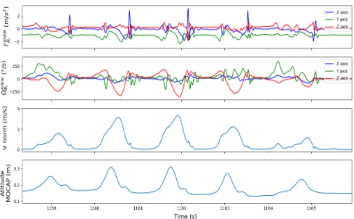
A group of people of various ages and heights, have practiced several activities (walking, running, stairs, side steps, small steps...) wearing the WATA system with infrared markers during motion capture (MOCAP) sessions under video control. The cameras record the position of the device with high pre-cision in a terrestrial reference frame defined at the beginning of the motion trial. Regarding the minimum of altitude and the video, we can detect when the foot is on the ground in the recording. Figure 3 illustrates a pattern in the inertial data that can be used to detect the beginning and the end of the strides during a walking phase. The contact of the foot with the ground is visible with a peak in the acceleration and a combination of conditions on the acceleration (one direction is close to one g, the two others are close to zero) and angular velocity (local minima, swing phase identification etc.) seems indeed to be sufficient criteria and presented good results in [18]. Nevertheless this method has shown its limits in situations of atypical movements such as fast sides stepping and rapid descent of stairs. Figure 4 exhibits the problem as it is hard to detect when a stride occurs from the inertial data.
Fig. 3: Pseudo-speed norm during walking.
Fig. 4: Pseudo-speed norm during fast side stepping.
On the contrary we can see in both Figure 3 and Figure 4 that the norm of V (Equation 14) is a good feature to solve this issue. The beginning and the end of a stride are defined by local minima around a maximum. However by following this procedure based on V norm criteria, many intervals are wrongly extracted when the wearer is moving its ankle but not walking. The goal is now to select among these intervals which ones are true strides. We adopt a statistical learning approach to answer this problem.
IV. ALGORITHM
A. Preprocessing and database
The first step of the algorithm is to project the inertial data in the terrestrial frame presented in Section II. Then we compute the pseudo-speed V described in Section III and defined in Equation 14. We saw in previous Section III that a combination of criteria on the norm of the computed speed allows to detect the start and the end of the stride. We set wide threshold values in order to detect all types of strides (small steps, running, stairs etc.). However many intervals are wrongly selected when the wearer is moving its ankle during daily activities other than walking (bicycling, sitting in a car etc.) and when the WATA system is manipulated before being worn on the ankle. Indeed, the sensors start recording when
the device is taken from its case and it can be carried with movement (in a backpack or pocket etc.) during an unknown amount of time. The goal is now to keep among these intervals those that are true strides. To answer this problem, we adopt a statistical learning approach.
From the intervals extraction above, a learning set is built from recordings of a group of people of various ages and heights practicing several activities. A binary label is affected to each interval indicating if it is a stride or not. Our database contains about 5000 positive intervals and also about 5000 negative intervals. In this binary classification problem, we adopt a strategy of supervised machine learning algorithm. B. Features engineering process
For all recordings, the inertial data and pseudo-speed are projected in the terrestrial frame Bterr whose the Zterr axis is aligned with the gravity and the two other axes (Xterrand Yterr) axes are set arbitrarily (Section II). To be robust to
this orientation that is dependent to each recording, in the following we compute a new rotation matrix around the Zterr
axis for all selected intervals.
Let the variable j in J1, N K denotes the index of each interval. These intervals are defined by one start and end that we note startjand endj. We assume that during the beginning
and the end of a stride, when the foot is flat on the floor, the ankle is in pure rotation. This mechanics is described in [19] and is illustrated in Figure 5. From this observation, if the
Fig. 5: The three foot rockers during stance phase. jth interval is a true stride we assume that the ankle speed at startj and endj is given by a lever arm:
V (startj) = ΩBterr(startj) ×
0 0 r ,
V (endj) = ΩBterr(endj) ×
0 0 r , (15)
with r the height relative to the ground of the device. In practice we set the value of r at 8 cm. From Equation 9 we can compute the forward speed (Vstartf or
j,endj) and the backward
speed (Vstartback
j,endj).
If the interval j is a stride, these two speeds are close because we integrate the acceleration during a short period so that the drift stays small. In practice, startj and endj do
not necessarily correspond to the ankle rocker. In addition, taking r equals 8 cm is not realistic for all recordings. That is why we observe differences in the residuals |Vstartf orj,endj(t) − Vback
startj,endj(t)| for t in [startj, endj]. However, it can be
much larger for movements that are not strides as Equation 15 do not stand.
Then, thanks to Equation 11, we compute Vstartj,endj(t)
on the studied interval. By integrating this pseudo-speed, we compute a pseudo-trajectory in the terrestrial reference frame Bterr, starting from the origin (0, 0, 0) and ending in
(xendj, yendj, zendj)
T: xendj yendj zendj = Z endj startj
Vstartj,endj(u)du. (16)
We consider a new terrestrial reference frame Bterr
j with the
Zterr
j axis still aligned with the gravity but with Xjterrdefined
by (xendj,yendj,zendj)
T
||(xendj,yendj,zendj)T||. We note R
terr
j the rotation matrix
that projects the data from Bterr to Bterr
j . For one stride
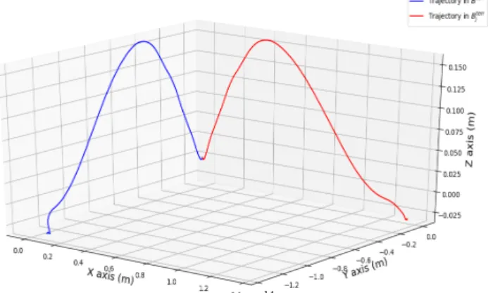
interval j, we plot the trajectories in Bterrand Bterr j (Figure
6). As we align the end of the trajectory with the Xterr j axis,
the value on Yterr
j of the end point is null. The body frames
Fig. 6: Example of a computed pseudo-trajectory in Bterrand Bterr
j .
Bterr
j are not the same for all j and for all recordings but
they have the same building specifications. The 3-D interval data we have access to (trajectory, pseudo-speeds, residuals, acceleration and angular velocity) in Bjterr are independent
to the initial position of the sensors. By proceeding this way We reduced drastically the complexity of the supervised learning problem. We compute features from signal processing techniques in time and frequency domains such as the mean, standard deviation, interquartile range, Fast Fourier Transform etc.
C. Gradient Boosting Tree algorithm
Following the strategy above, for each element of our database, 1657 features are computed. We want to build a binary classifier that decides if one interval is a stride. Several supervised statistical learning algorithms have been tested, notably random forests which are known to perform well in large dimensions, Support Vector Machine (SVM), LASSO regression and boosting algorithms such as Adaboost and GBT (Gradient Boosting Tree [20]). We evaluated their performance using the cross-validation method (10-fold cross-validation [21]). The chosen algorithm with the best results is GBT.
The general idea is to compute a series of (very weak) decision trees [22], learning at each step the prediction error of the previous aggregation. Let {(X1, Y1), . . . , (Xq, Yq), . . . (XN, YN)} the elements of
our database. As we computed 1657 features we have Xq in R1657. We note Yq the binary label of the interval
(Yq ∈ {0, 1}). We introduce X = (X1, . . . , XN) and
Y = (Y1, . . . , YN) for describing the GBT algorithm in the
following.
Algorithm 1: GBT algorithm
Input : Initial prediction: pred0(X) ∈ R(N ×1657)
Learning rate constant : c ∈R Number of iterations : K ∈ N Output: Prediction function
1 for k = 1, . . . , K do
2 Compute the error: errork(X) = Y − predk−1(X) 3 Fit the weak decision tree fkon (X, errork(X))
4 Udapte the prediction: predk(X) = predk−1(X) + c fk(X) 5 end
The parameters c and K have to be tuned to avoid the overfitting. They have been set by cross-validation.
D. Overview
Algorithm 2: Algorithm of the trajectory reconstruction
Input : Recording of the system worn at the ankle Output: Trajectory of the system
1 Projection of the inertial data in a terrestrial reference frame (Section II)
2 Detection of inactivity {(t01, t11), . . . , (t0i, t 1 i), . . . , (t
0 n, t1n)} 3 Pseudo-speed computation (Section III)
4 foreach ankle movement period i do
5 Extraction of candidate stride intervals 6 foreach interval j do
7 Data alignment (Section IV-B)
8 Features computation
9 GBT binary classification for stride detection
10 if interval classified as a stride then
11 ZUPT on the start and the end of the interval
12 Data integration between the two ZUPTs 13 Pseudo-speed update: V (t) = Vendj,t1i(t),
∀t ∈ [endj, t1i] (Equation 11)
14 Update of the posterior candidate stride intervals extraction
15 end 16 end
17 end
The step 13 of the Algorithm 2 is important to counter the integration drift if the ankle movement period [t0
i, t1i] is
large. In that case, the weighted mean of forward speed and backward speed (Equations 10 and 11) may not overtake the integration errors for t far from t0
i and t1i. With the
pseudo-speed update if strides are detected, the weighted mean is computed for smaller and smaller interval and overcomes the integration drift.
V. APPLICATIONS
The following section describes the performance of the stride detection and experimental results demonstrating the accuracy of the position estimation using the Algorithm 2.
A. Stride detector performance
1) Performance on the database: The database contains 5779 intervals that do not correspond to strides (label 0) and 4870 stride intervals divided into different activities: "atypical step" that includes small step, side step, backward walking etc., walking, running, climbing and descending stairs. The label 0 intervals come from ankle movement that are not strides during bicycling for example and situations when the device is manipulated in the hand, carried in a pocket or backpack before being worn on the ankle. The cross-validation results using GBT are presented in the following confusion matrix (Table I).
Predicted 0 Predicted 1
Actual 0 5659 120
Actual 1 191 4679
TABLE I: Confusion matrix of GBT algorithm. The mean error is less than 0.3%. This score depends on the difficulty of the database. A lot of atypical strides and ankles movements (labelled -1) that look like true stride from inertial data point of view have been included in the database. As a result, the final score is slightly deteriorated but it leads to more robust classifier.
2) Performance in MOCAP sessions: That is why we also tested our algorithm on 7 MOCAP sessions. The stride intervals detected are manually validated with the video and the MOCAP altitude. The foot has to be on the ground to accept the detection. We ask the wearers to walk at three different paces, small steps and side steps (both sides). In order to observe left and right turns and straight lines, the wearers had to follow a loop path in both directions and an eight-shape reference trajectory. The results are presented in Table II and III.
Slow walking Medium walking Fast walking Total Detected Total Detected Total Detected Wearer 1 291 291 - 100% 279 279 - 100% 216 216 - 100% Wearer 2 306 306 - 100% 261 261 - 100% 195 195 - 100% Wearer 3 294 294 - 100% 219 219 - 100% 198 198 - 100% Wearer 4 297 297 - 100% 267 267 - 100% 228 228 - 100% Wearer 5 273 273 - 100% 249 249 - 100% 213 213 - 100% Wearer 6 345 345 - 100% 339 339 - 100% 327 327 - 100% Wearer 7 342 342 - 100% 246 246 - 100% 240 240 - 100% Total 2148 2148 - 100% 1860 1860 - 100% 1617 1617 - 100%
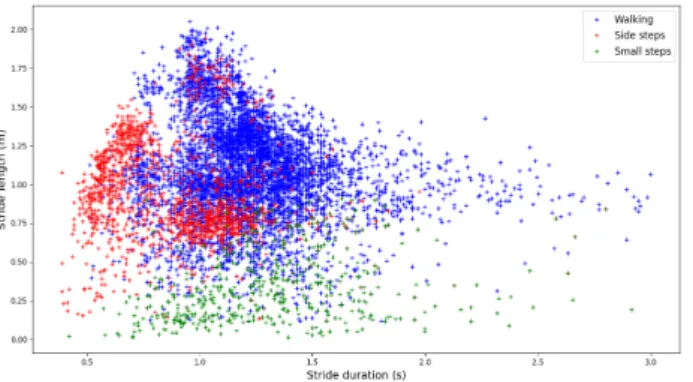
TABLE II: Detection rate for walking phases. All walking strides are detected. We can see on Figure 7 that the MOCAP database present diversified stride lengths and stride durations. It means our detection achieves 100% accuracy for walking phases with various paces. Some of the
Fig. 7: Stride lengths as a function of stride durations.
walking strides may appear very small but it is due to half turns of the MOCAP sessions. The foot comes in the end very close to the starting point of the stride.
Small steps Side steps Total Detected Total Detected Wearer 1 88 88 - 100% 287 285 - 99.3% Wearer 2 67 67 - 100% 265 258 - 97.4% Wearer 3 107 102 - 95.3% 143 138 - 96.5% Wearer 4 145 144 - 99.3% 301 301 - 100% Wearer 5 65 62 - 92.3% 246 244 - 99.2% Wearer 6 90 89 - 98.9% 150 149 - 99.3% Wearer 7 48 44 - 91.7% 200 199 - 99.5% Total 610 596 - 97.7% 1592 1574 - 98.9%
TABLE III: Detection rate for atypical strides. Our algorithm does not detect all atypical strides but shows good results while most existing methods described in the literature do not detect them.
B. Trajectory reconstruction performance
1) Performance in MOCAP sessions: We first study the trajectory reconstruction performance by comparing the stride length computed by our algorithm to the MOCAP reference during sessions introduced in Section III-B. The results are presented in Tables IV and V.
Slow walking Medium walking Fast walking Mean (m) Std (m) Mean (m) Std (m) Mean (m) Std (m)
Wearer 1 0.024 0.038 0.020 0.022 0.029 0.036 Wearer 2 0.026 0.039 0.016 0.018 0.025 0.034 Wearer 3 0.023 0.021 0.028 0.024 0.036 0.023 Wearer 4 0.028 0.020 0.028 0.021 0.023 0.022 Wearer 5 0.061 0.091 0.025 0.020 0.032 0.029 Wearer 6 0.018 0.016 0.024 0.024 0.043 0.039 Wearer 7 0.014 0.026 0.014 0.012 0.023 0.044 Total 0.028 0.048 0.022 0.021 0.032 0.034
TABLE IV: Absolute computed stride length error for walking phases.
Small steps Side steps Mean (m) Std (m) Mean (m) Std (m) Wearer 1 0.027 0.070 0.044 0.106 Wearer 2 0.039 0.048 0.071 0.168 Wearer 3 0.057 0.082 0.070 0.177 Wearer 4 0.025 0.024 0.048 0.056 Wearer 5 0.049 0.082 0.022 0.046 Wearer 6 0.074 0.061 0.133 0.170 Wearer 7 0.039 0.055 0.053 0.116 Total 0.048 0.069 0.056 0.129
TABLE V: Absolute computed stride length error for atypical strides.
Our algorithm achieves similar performances than existing methods ( [23], [24]) for normal walking but also good performances for atypical strides (around 5 cm of absolute mean error) that are not even studied in the literature.
2) Performance in non controlled environment: In the fol-lowing we validate the trajectory reconstruction in an everyday life situation. For this test an office worker has worn the system during 5 hours and 30 minutes. The aim is to test the step detector algorithm on strides performed naturally, including small steps. During those 5 hours and 30 minutes, the person was mostly sitting on his office chair. These periods are also interesting because the ankle does not remain inactive and it is important that no stride is wrongly detected. The recording
contains 3 walking periods including up and down stairs in the first and last one.
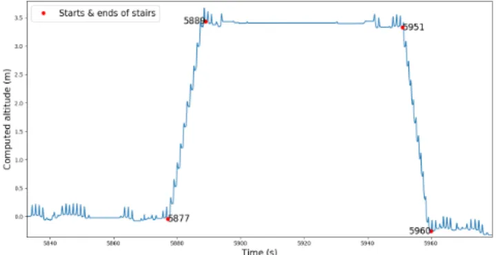
The computed altitude of the first walking period is rep-resented in Figure 8. From this graph we can detect when
Fig. 8: Computed altitude during the first walking period. the wearer is walking in the stairs. We plot in Figure 9 the computed trajectory in two dimensions on the plans of the ground floor and first floor depending on this altitude evolution. We add markers that indicate the beginning/end of the detected stairs from Figure 8 above. The colormap defines the time over the considered walking period: the more the greyscale is dark the more time has elapsed. In addition, the starting point is initialized with the coordinates (0, 0, 0) and the computed trajectory has been rotated to have the correct initial direction.
Fig. 9: Computed trajectory during the first walking period on the ground floor (left) and first floor (right).
During the second walking period, the wearer stays on the first floor. We plot in two dimensions the computed trajectory on the corresponding plan in Figure 10.
Fig. 10: Computed trajectory dur-ing the second walkdur-ing period on the ground floor.
The computed altitude of the third walking period is rep-resented in Figure 11. Using the same first walking period
Fig. 11: Computed altitude during the third walking period.
approach, we plot in Figure 12 the computed trajectory in two dimensions and we add markers that indicate the begin-ning/end of the detected stairs from Figure 11 above. This
Fig. 12: Computed trajectory during the third walking period on the ground floor (left) and the first floor (right).
experiment illustrates the good performance of the trajectory reconstruction in a difficult environment with narrow ways, small rooms and corridors. In this context, the computed trajectory almost never crosses the walls and we can identify in what room the wearer is at any time or when he is taking the stairs. Figure 8 and Figure 11 indicate a difference in the computed altitude of 3.4 meters for both stairs phases that are composed of 21 stair-treads of 15.4 cm height. The true altitude of the first ground is 3.234 meters so the altitude mean error is less than 1 cm for each stair-tread. In addition, the starting point of the second and third walking period correspond to the ending point of the previous one. It means that no stride is wrongly detected when the wearer is on his chair and moving his ankle.
VI. CONCLUSION
This paper describes an algorithm that compute the trajec-tory of a pedestrian wearing an ankle worn inertial device. This work is divided in four main steps:
• The projection of the inertial data in a terrestrial reference frame by detecting the gravity in the accelerations.
• The extraction of candidate intervals based on the com-puted pseudo-speed that may correspond to strides.
• The binary classification of the intervals using the Gra-dient Boosting Tree algorithm.
• The computation of an inspired ZUPT technique for the
detected stride.
For normal walking it shows good results achievable with existing algorithms with 100% stride detection rate and around 3 cm of absolute mean error for the stride length. In addition, the method described in this paper also has a good sensitivity for atypical strides such as small steps, side steps contrary to most algorithms proposed in the literature. It achieves more than 98% detection rate and the absolute mean error of the stride length is about 5 cm.
Moreover existing approaches are likely to produce detec-tion error when the system wearer is moving his ankle but not walking (e.g. sitting). This is a problem as non walking motion would be integrated erroneously in the trajectory. Our algorithm handles those situations without false detection. A challenging test have been performed by recording an office worker during 5 hours and 30 minutes. The building presented narrow areas and stairs forcing the wearer to perform atypical steps. He stayed also for several hours sitting on his chair keeping his ankle moving. In this context, the computed trajectory illustrates the good performance by barely never crossing the walls of the building map and no stride is wrongly detected as false positive.
ACKNOWLEDGMENT
This work was supported by the French Délégation Générale de l’Armement (DGA) and by ANR project TopData ANR-17-MALN-0003.
REFERENCES
[1] Y. Chen and H. Kobayashi, “Signal strength based indoor geolocation,” Proceedings of the IEEE International Conference on Communications, pp. 436–439, 2002.
[2] V. Renaudin, “Uwb and mems based indoor navigation,” The Journal of Navigation, vol. 61, pp. 369–384, 2008.
[3] S. S. et al., “Hybrid localization using uwb and inertial sensors,” IEEE Int. Conf. Ultra-Wideband (ICUWB), pp. 89–92, 2008.
[4] E. Dorveaux, “Magneto-inertial navigation: principles and application to an indoor pedometer,” PhD thesis, École Nationale Supeure des Mines de Paris, 2011.
[5] C. I. Chesneau, M. Hillion, and C. Prieur, “Motion estimation of a rigid body with an ekf using magneto-inertial measurements,” Indoor Positioning and Indoor Navigation (IPIN), 2016.
[6] K. Abdulrahim, T. Moore, C. Hide, and C. Hill, “Understanding the performance of zero velocity updates in mems-based pedestrian navi-gation,” International Journal of Advancements in Technology, vol. 5, no. 2, 2014.
[7] E. Foxlin, “Pedestrian tracking with shoe-mounted inertial sensors,” IEEE Computer graphics and applications, pp. 38–46, 2005.
[8] A. M. Sabatini, “Quaternion-based strap-down integration method for applications of inertial sensing to gait analysis,” Medical and Biological Engineering and Computing, pp. 94–101, 2005.
[9] S. J. Bamberg, A. Y. Benbasat, D. M. Scarborough, E. E. Krebs, and J. A. Paradiso, “Gait analysis using a shoe-integrated wireless sensor system,” IEEE transactions on information technology in biomedicine, pp. 413–423, 2008.
[10] M. Susi, V. Renaudin, and G. Lachapelle, “Motion mode recognition and step detection algorithms for mobile phone users,” Sensors, pp. 1539– 1562, 2013.
[11] B. Florentino-Liano, N. O’Mahony, and A. Artes-Rodriguez, “Human activity recognition using inertial sensors with invariance to sensor orientation,” Conf. Cognitive Information Processing (CIP), 2012. [12] S. Ghose, J. Mitra, M. Karunanithi, and J. Dowling, “Human activity
recognition from smart-phone sensor data using a multi-class ensemble learning in home monitoring,” Stud Health Tehcnol Inform, 2015.
[13] N. Castaneda and S. Lamy-Perbal, “An improved shoe-mounted inertial navigation system,” International conference on indoor positioning and indoor navigation (IPIN), 2010.
[14] J.-L. Carrera, Z. Zhao, T. Braun, and Z. Li, “A real-time indoor tracking system by fusing inertial sensor, radio signal and floor plan,” International conference on indoor positioning and indoor navigation (IPIN), 2016.
[15] A. Norrdine, Z. Kasmi, and J. Blankenbach, “Step detection for zupt-aided inertial pedestrian navigation system using foot-mounted perma-nent magnet,” International conference on indoor positioning and indoor navigation (IPIN), 2016.
[16] T. Moder, K. W. nd P. Hafner, and M. Wieser, “Smartphone-based indoor positioning utilizing motion recognitiont,” International conference on indoor positioning and indoor navigation (IPIN), 2015.
[17] S. Y. Cho and C.-G. Park, “Mems based pedestrian navigation system,” Journal of Navigation, vol. 59, pp. 135–153, 2006.
[18] B. Beaufils, F. Chazal, M. Grelet, and B. Michel, “Stride detection for pedestrian trajectory reconstruction: a machine learning approach based on geometric patterns,” International conference on indoor positioning and indoor navigation (IPIN), 2017.
[19] Z. O. Abu-Faraj, G. F. H. andPeter A Smith, and S. Hassani, “Human gait and clinical movement analysis,” Wiley Encyclopedia of Electrical and Electronics Engineering, 2015.
[20] J. H. Friedman, “Computational statistics and data analysis,” 2002. [21] M. Stone, “Cross-validatory choice and assessment of statistical
predic-tions,” Journal of the Royal Statistical Society, pp. 111–147, 1974. [22] L. Breiman, J. Friedman, R. Olshen, and C. Stone, “Classification and
regression tree,” 1984.
[23] N.-H. Ho, P. H. Truong, and G.-M. Jeong, “Step-detection and adaptive step-length estimation for pedestrian dead-reckoning at various walking speeds using a smartphone,” Sensors, 2016.
[24] J. Hannink, C. F. P. Thomas Kautz, J. Barth, S. Schlein, K.-G. G. mann, J. Klucken, and B. M. Eskofier, “Stride length estimation with deep learning,” IEEE EMBS, 2017.