HAL Id: hal-00685002
https://hal.inria.fr/hal-00685002v2
Submitted on 19 Aug 2012
HAL is a multi-disciplinary open access
archive for the deposit and dissemination of
sci-entific research documents, whether they are
pub-lished or not. The documents may come from
teaching and research institutions in France or
abroad, or from public or private research centers.
L’archive ouverte pluridisciplinaire HAL, est
destinée au dépôt et à la diffusion de documents
scientifiques de niveau recherche, publiés ou non,
émanant des établissements d’enseignement et de
recherche français ou étrangers, des laboratoires
publics ou privés.
Analysis-suitable volume parameterization of multi-block
computational domain in isogeometric applications
Gang Xu, Bernard Mourrain, Régis Duvigneau, André Galligo
To cite this version:
Gang Xu, Bernard Mourrain, Régis Duvigneau, André Galligo. Analysis-suitable volume
param-eterization of multi-block computational domain in isogeometric applications.
Computer-Aided
Design, Elsevier, 2013, Special Issue on Solid and Physical Modeling 2012, 45 (2), pp.395-404.
�10.1016/j.cad.2012.10.022�. �hal-00685002v2�
Analysis-suitable volume parameterization of multi-block computational
domain in isogeometric applications
Gang Xu
aBernard Mourrain
bR´egis Duvigneau
bAndr´e Galligo
caSchool of Computer Science and Technology, Hangzhou Dianzi University, Hangzhou 310018, P.R.China bINRIA Sophia-Antipolis, 2004 Route des Lucioles, 06902 Cedex, France
cUniversity of Nice Sophia-Antipolis, 06108 Nice Cedex 02, France
Abstract
Parameterization of computational domain is a key step in isogeometric analysis just as mesh generation is in finite element analysis. In this paper, we study the volume parameterization problem of multi-block computational domain in isogeometric version, i.e, how to generate analysis-suitable parameterization of the multi-block computational domain bounded by B-spline surfaces. Firstly, we show how to find good volume parameterization of single-block computational domain by solving a constraint optimization problem, in which the constraint condition is the injectivity sufficient conditions of B-spline volume parametrization, and the optimization term is the minimization of quadratic energy functions related to the first and second derivatives of B-spline volume parameterization. By using this method, the resulted volume parameterization has no self-intersections, and the isoparametric structure has good uniformity and orthogonality. Then we extend this method to the multi-block case, in which the continuity condition between the neighbor B-spline volume should be added to the constraint term. The effectiveness of the proposed method is illustrated by several examples based on three-dimensional heat conduction problem.
Key words: isogeometric analysis, volume parameterization, multi-block computational domain, heat conduction
1. Introduction
Isogeometric analysis (IGA for short) method pro-posed by Hughes et al. in [16] offers the possibility of bridg-ing the gap between CAD and CAE. The approach uses the same spline representation both for the geometry and for the physical solutions, and thus avoids this costly forth and back transformations. This uniform framework pro-vides more accurate and efficient ways to deal with com-plex shapes and to approximate the solutions of physical simulation problems. On the other hand, it also rises inter-esting geometric problems for analysis-suitable modeling tools [23][22] [24].
It is well known that mesh generation, which generates a discrete mesh of a computational domain from a given CAD object, is a key and the most time-consuming step in finite element analysis (FEA for short). It consumes about 80% of the overall design and analysis process [4] in
automo-Email addresses: [email protected] (Gang Xu), [email protected](Bernard Mourrain), [email protected] (R´egis Duvigneau), [email protected](Andr´e Galligo).
tive, aerospace and ship industry. Parametrization of com-putational domain in IGA, which corresponds to the mesh generation in FEA, also has some impact on analysis result and efficiency. In particular, arbitrary refinements can be performed on the computational mesh in FEA, but in IGA if we compute with tensor product B-splines, we can only perform refinement operations in each parametric direction by knot insertion or degree elevation. Hence, parameteri-zation of computational domain is also being important for IGA. As it is pointed by Cottrell et al.[6], one of the most significant challenges towards isogeometric analysis is con-structing trivariate spline volume parameterizations from given CAD boundary representation.
From the viewpoint of graphics applications, vol-ume parameterization of 3D models has been studied in [17,26,25]. As far as we know, there are only a few work on the parametrization of computational domains from the viewpoint of isogeometric applications. T. Martin et al. [18] proposed a method to fit a genus-0 triangular mesh by B-spline volume parameterization, based on dis-crete volumetric harmonic functions; this can be used to build computational domains for 3D IGA problems. E. Cohen et.al. [7] proposed the concept of analysis-aware
modeling, in which the parameters of CAD models should be selected to facilitate isogeometric analysis. They also demonstrated the influence of parameterization of com-putational domains by several examples. J.M Escobar et al. proposed a method to construct a trivariate T-spline volume of complex genus-zero solids for isogeometric ap-plication [12]. However, the proposed method demands a surface triangulation as input data. A variational approach for constructing NURBS parameterization of swept vol-umes is proposed by M. Aigner et al [1]. Given boundary CAD information, approximate implicitization technique is used for parametrization of 2D computational domain in [20]. In [27][28], r-refinement method for generating optimal analysis-aware parameterization of computational domain is proposed. However, it only works for speci-fied analysis problems. A general construction method for analysis-suitable planar B-spline parameterization in two-dimensional isogeometric problem is proposed in [29] based on harmonic mapping. In this paper, from the given boundary CAD information, the volume parameterization problem for multi-block computational domain is stud-ied based on the trivariate generalization of the method proposed in [28].
In IGA, the parameterization of a computational do-main is determined by control points, knot vectors and the degrees of B-spline objects. For three-dimensional IGA problems, the knot vectors and the degree of the com-putational domain are determined by the given boundary surfaces. That is, given boundary surfaces, the quality of parameterization of computational domain is determined by the positions of inner control points. Hence, finding a good placement of the inner control points inside the com-putational domain, is a key issue. A basic requirement of the resulting volume parameterization for IGA is that it doesn’t have self-intersections, so that it is an injective map from the parametrization domain to the computa-tional domain. In order to get more accurate simulation results, the isoparametric structure in the computational domain should be as uniform as possible and have orthog-onal isoparametric surfaces [2]. In this paper, we study the volume parameterization problem of multi-block computa-tional domain in isogeometric version, i.e, how to generate analysis-suitable parameterization of the multi-block com-putational domain bounded by B-spline surfaces. Our main contributions are:
– A constraint optimization framework is proposed to generate a multi-block volume parameterization with-out self-intersections, and the resulted isoparametric structure has good uniformity and orthogonality; – Some classical results in the field of differential geometry
related to parametric surfaces are generalized to the case of trivariate parametric volumes, such as the orthogonal conditions of isoparametric structure and the C1 condi-tions between B-spline volumes.
– We test the volume parameterization results on heat con-duction problem to show the effectiveness of the proposed method.
The remainder of the paper is organized as follows. Section 2 presents some preliminary on B-spline volume parameterization. Section 3 describes the constraint opti-mization method for single-block volume parameterization of 3D computational domain. Section 4 presents a volume parameterization framework for multi-block computational domain based on the proposed methods in Section 3. Sec-tion 5 tests the volume parameterizaSec-tion results on heat conduction problem to show the effectiveness of the pro-posed method. Finally, we conclude this paper in Section 6. 2. Preliminary
For a parameterization σ from P : [a, b] × [c, d] × [e, f ] to Ω ⊂ R3, we define the boundary surfaces as the image of {a}×[c, d]×[e, f ], {b}×[c, d]×[e, f ],{c}×[a, b]×[e, f],{d}× [a, b] × [e, f ], {e} × [a, b] × [c, d], {f } × [a, b] × [c, d] by σ. We say that σ defines a regular boundary if these surfaces do not intersect pairwise, except at their boundary curves and if they have no self-intersection points.
We consider the following trivariate B-spline parame-terization σ : (ξ, η, ζ) ∈ P : = [a, b] × [c, d] × [e, f ] 7→ σ(ξ, η, ζ) : = X 0≤i≤l 0≤j≤m 0≤k≤n ci,j,kNip(ξ)Njq(η)Nkr(ζ),
where ci,j,k∈ R3are the control points, Nip(ξ), N q j(η) and Nr
k(ζ) are B-spline functions of degree p, q and r for a given knot vector on [a, b], [c, d] and [e, f ] . Note that in this paper we use knot vectors with multiple end knots to forces the volumes to interpolate the corner control points.
The derivative of σ(ξ, η, ζ) with respect to ξ can be expressed in terms of the differences ∆1
i,j,k := (∆1,xi,j,k, ∆1,yi,j,k, ∆1,zi,j,k) = ci+1,j,k− ci,j,k:
∂ξσ = X 0≤i≤l−1 0≤j≤m 0≤k≤n ω1 i,j,k∆ 1 i,j,kN p−1 i (ξ)N q j(η)Nkr(ζ), (1)
where Nip−1(ξ) is the B-spline function with one degree less in u, ω1
i,j,kis a positive factor.
Similarly, the derivative of σ(ξ, η, ζ) with respect to η and ζ can be expressed as follows
∂ησ = X 0≤i≤l 0≤j≤m−1 0≤k≤n ω2i,j,k∆ 2 i,j,kN p i(ξ)N q−1 j (η)N r k(ζ), (2) ∂ζσ = X 0≤i≤l 0≤j≤m 0≤k≤n−1 ωi,j,k3 ∆ 3 i,j,kN p i(ξ)N q j(η)N r−1 k (ζ), (3) where ∆2 i,j,k= (∆ 2,x i,j,k, ∆ 2,y i,j,k, ∆ 2,z
i,j,k) = ci,j+1,k− ci,j,k, ∆3i,j,k= (∆ 3,x i,j,k, ∆ 3,y i,j,k, ∆ 3,z
i,j,k) = ci,j,k+1− ci,j,k, and ω2
2.1. Non-linear sufficient condition based on Jacobian computation
From [28], if the Jacobian determinant J (σ(ξ, η, ζ)) of trivariate B-spline parameterization satisfies J (σ(ξ, η, ζ)) > 0, then σ(ξ, η, ζ) has no self-intersections.
From (1), (2), (3) and the product properties of splines [19] , the Jacobian determinant J (σ(ξ, η, ζ)) of B-spline surface can be computed as follows:
J(σ(ξ, η, ζ)) = σxξ σηx σζx σξy σyη σ y ζ σz ξ σzη σζz = X 0≤i≤l−1 0≤j≤m 0≤k≤n X 0≤i′≤n 0≤j′≤m−1 0≤k′≤n X 0≤i′′≤n 0≤j′′≤m 0≤k′′≤n−1 Nip−1(ξ)Njq(η)Nr k(ζ) Nip′(ξ)N q−1 j′ (η)N r k′(ζ) N p i′′(ξ)N q j′′(η)N r−1 k′′ (ζ) ω1 i,j,kω 2 i′,j′,k′ω 3 i′′,j′′,k′′
∆1,xi,j,k ∆2,xi,j,k ∆3,xi,j,k ∆1,yi′,j′,k′ ∆ 2,y i′,j′,k′ ∆ 3,y i′,j′,k′ ∆1,zi′′,j′′,k′′ ∆ 2,z i′′,j′′,k′′ ∆ 3,z i′′,j′′,k′′ = 3l−1 X i=0 3m−1 X j=0 3n−1 X k=0 GijkNi3p−1(ξ)N 3q−1 i (η)N 3r−1 k (ζ) (4) Hence, the Jacobian of trivariate B-spline parameteri-zation can be represented in the form of trivariate B-spline volume with higher degrees. From the convex hull property of B-splines [13], we have the following theorem.
Theorem 2.1 If Gijk > 0 in (4), then J(σ(ξ, η, ζ)) > 0, that is, σ(ξ, η, ζ) has no self-intersections.
This is a non-linear sufficient condition with respect to the inner control points. We will use it as constraint term in the constraint optimization method for volume generation in Section 3.
2.2. Linear constraint for injectivity.
In order to be self-contained, the linear sufficient con-dition proposed in [27] for injectivity of a B-spline volume parameterization is presented in this subsection.
We denote by Ci the convex cone of Ri generated by the half rays R+·
∆ii,j,k k∆i
i,j,kk
, i = 1, 2, 3. If this cone is generated by two opposite vectors, which are on a straight line, we define Ci(c) as any half-plane. We say that two cones C1, C2 are transverse if R · C1and R · C2intersect only at {0}. We say that three cones C1, C2, C3are cotransverse if
– 0 is a vertex of the convex hull of C1, C2, C3;
– the convex hull of the cones Ci, Cj and the cone Ck are transverse for all {i, j, k} = {1, 2, 3}.
Given six boundary surfaces described by the controls points ci,0,k, ci,l2,k, c0,j,k, cl1,j,k, ci,j,0, ci,j,l3, with 0 ≤ i ≤
l1, 0 ≤ j ≤ l2, 0 ≤ k ≤ l3, we define the boundary cone C10
O H1 O1 O2 O3 T12 M12 T21 T23 M23 T32 T31 M13 T13 H3 H2
Fig.1. Construction of constraint plane.
(resp. C0
2, C30) as the cone generated by the vectors ∆1i,j,0(c), ∆1
i,j,l3(c) for 0 ≤ i ≤ l1− 1, 0 ≤ j ≤ l2 (resp. ∆
2 0,j,k(c), ∆2 l2,j,k(c) for 0 ≤ j ≤ l2−1, 0 ≤ k ≤ l3, ∆ 3 i,0,k(c), ∆3i,l2,k(c)
for 0 ≤ i ≤ l1, 0 ≤ k ≤ l3− 1). We assume that these boundary surfaces form a regular boundary and that the three boundary cones C0
1, C 0 2, C
0
3are cotransverse. Then we can find
– a plane H0such that ∀u ∈ Ci0,∗(i = 1, 2, 3), H0(u) > 0, and
– a plane Hk such that ∀u ∈ Ci0,∗∪ C 0,∗
j , Hk(u) > 0 and ∀u ∈ C0,∗k , Hk(u) < 0 for {i, j, k} = {1, 2, 3}.
Such separating planes can be deduced easily from convex hull computations of finite sets of vectors, which are gen-erating the cones C0
1, C 0 2, C
0
3 or their unions.
As shown in Fig.1, suppose that O is the origin, O1, O2and O3are the center of the circular cone C01(c),C20(c) and C0
3(c), respectively. The great-circle arc connecting O1 and O2intersects the circular cone C10(c) and C20(c) at T12 and T21. We can construct a orthogonal plane H1of plane OT12T21through OM12, where M12is the middle points of T12T21. Let F12be the linear equation defining the plane H1. Then the vectors in C10(c) and C20(c) satisfy F12 ≤ 0 and F12≥ 0 respectively. Similarly, we can define F13and F23as the linear equations defining the plane H2and H3. Based on above the construction, the linear constraint conditions of inner control points for injective trivariate B-spline parameterization can be presented as follows,
H0(ci+1,j,k− ci,j,k) > 0, H1(ci+1,j,k− ci,j,k) < 0, H2(ci+1,j,k− ci,j,k) > 0, H3(ci+1,j,k− ci,j,k) > 0, H0(ci,j+1,k− ci,j,k) > 0, H1(ci,j+1,k− ci,j,k) > 0, H2(ci,j+1,k− ci,j,k) < 0, H3(ci,j+1,k− ci,j,k) > 0, H0(ci,j,k+1− ci,j,k) > 0, H1(ci,j,k+1− ci,j,k) > 0, H2(ci,j,k+1− ci,j,k) > 0, H3(ci,j,k+1− ci,j,k) < 0,
(5) where 0 < i < l1, 0 ≤ j < l2, 0 ≤ k < l3.
This set of conditions provides linear constraints for the injectivity of trivariate B-spline volume parameteriza-tion. In the following section, it will be used as constraint term in the quadratic programming method for the case
when the boundary cones are cotransverse.
Remark 1. Note that the above two sufficient conditions only ensures the injectivity locally. The global injectivity can be guaranteed by the regularity of given boundary sur-faces.
3. Constraint optimization method for volume parametrization of computational domains
In this section, we aim at finding injective volume pa-rameterization of the computational domain with a uni-form and orthogonal isoparametric net.
3.1. Initial construction of inner control points
In order to solve this constraint optimization problem, an initial construction of inner control points is required. We rely on the discrete Coons method to generate inner control points as initial value from boundary control points, which can be considered as the trivariate generalization of the method presented in [14].
Suppose that given boundary surfaces are B-spline surfaces, the opposite boundary B-B-spline sur-faces have the same degree, number of control points and knot vectors. Given the boundary control points c0,j,k, cl,j,k, ci,0,k, ci,m,k, ci,j,0, ci,j,n, (i = 0, . . . , l, j = 0, . . . , m, k = 0, . . . , n ), then the interior control points ci,j,kcan be constructed as follows,
ci,j,k= (1 − i/l)c0,j,k+ i/lcl,j,k+ (1 − j/m)ci,0,k +j/mci,m,k+ (1 − k/n)ci,j,0+ k/nci,j,n
−[1 − i/l, i/l] c0,0,k c0,m,k cl,0,k cl,m,k 1 − j/m j/m −[1 − j/m, j/m] ci,0,0 ci,0,n ci,m,0 ci,m,n 1 − k/n k/n −[1 − k/n, k/n] c0,j,0 cl,j,0 c0,j,n cl,j,n 1 − i/l i/l +(1 − k/n) [1 − i/l, i/l] c0,0,0 c0,m,0 cl,0,0 cl,m,0 1 − j/m j/m +k/n [1 − i/l, i/l] c0,0,n c0,m,n cl,0,n cl,m,n 1 − j/m j/m
Then the corresponding B-spline volume has the following form σ(ξ, η, ζ) = l X i=0 m X j=0 n X k=0 ci,j,kNi(ξ)Nj(η)Nk(ζ). where Ni(ξ), Nj(η) and Nk(ζ) are B-spline function with knot vectors given by boundary surfaces.
(a) Isoparametric surfaces and curves in a trivariate B-spline volume
(b) The partial derivatives at a point inside the volume
Fig.2. Isoparametric structure and partial derivatives in the trivari-ate B-spline parameterization.
This initial construction of inner control points can be considered as an extension of boolean sum of ruled vol-umes and trilinear volvol-umes constructed from give bound-ary surfaces as proposed in [11] . The resulting inner con-trol points lie in the convex hull of the boundary concon-trol points as the sum of the coefficients equals 1. For some given boundary surfaces, this construction may cause some self-intersections, and lead to an improper volume param-eterization for IGA.
3.2. Trivariate parametric volume with orthogonal and uniform grid
An internal energy function of the computational do-main will be used as an optimization term in a constraint optimization method to construct a computational domain with an uniform and orthogonal isoparametric grid.
In a trivariate B-spline parametrization, it has isopara-metric surfaces and isoparaisopara-metric curves with B-spline form as shown in Fig. 2(a). The partial derivatives at a point inside the trivariate volume are also shown in Fig. 2(b). For the trivariate parametric volume with orthogonal isoparametric surfaces, we have the following proposition. Proposition 3.1 A trivariate parametric volume σ(ξ, η, ζ) has isoparametric grid with orthogonal isoparametric sur-faces if and only if it satisfies the following condition
σξ· ση = σξ· σζ = ση· σζ = 0 (6) The above proposition indicates that a trivariate para-metric volume has orthogonal isoparapara-metric surfaces if and only if each isoparametric surface has orthogonal isopara-metric net.
By minimizing the following energy functions, one can achieve isoparametric grid with orthogonal isoparametric surfaces,
Z Z
|σξ· ση| + |σξ· σζ| + |ση· σζ|dξdηdζ. (7) In view of the following inequalities,
|σξ· ση| ≤ k σξ k2+ k ση k2 2 |σξ· σζ| ≤ k σξ k2+ k σζ k2 2 |ση· σζ| ≤ k ση k2+ k σζ k2 2 we replace (7) with Z Z Z k σξ k2+ k ση k2+ k σζ k2dξdηdζ. (8) The energy functions (8) can be seen as the trivariate gen-eralization of stretch energy in [5]. The strain energy of parametric surface is related to the uniformity of the iso-parameteric net as shown in [5]. Then we can generalize the strain energy in trivariate form as follows:
Z Z Z
(k σξξ k2+ k σηηk2+ k σζζk2 (9) +2 k σξη k2+2 k σξζk2+2 k σηζ k2)dξdηdζ.
In summary, combining (8) and (9), we use the follow-ing optimization term as objective function,
min Z Z Z
(k σξk2+ k σηk2+ k σζ k2) +ω(k σξξ k2+ k σηηk2+ k σζζk2
+2 k σξη k2+2 k σξζk2+2 k σηζ k2)dξdηdζ. where ω is a positive constant.
3.3. Non-linear constraint optimization method for volume parameterization
After introducing the quadratic energy function in subsection 3.2, the following constraint optimization algo-rithm can be obtained based on the non-linear sufficient condition in subsection 2.1:
Input: six boundary B-spline surfaces
Output: inner control points and the corresponding B-spline volume parameterization
– Construct the initial inner control points as in subsection 3.1;
– Construct the constraint condition (4) from boundary B-spline surfaces as in Section 2;
– Solve the following constraint optimization problem by using sequential quadratic programming (SQP for short) method min Z Z Z (k σξ k2+ k ση k2+ k σζ k2) +ω(k σξξ k2+ k σηηk2+ k σζζk2 +2 k σξηk2+2 k σξζ k2+2 k σηζ k2)dξdηdζ. s.t. Gijk> 0
– Generate the corresponding B-spline volume parameter-ization σ(ξ, η, ζ) as computational domain.
Remark 2. SQP is an iterative procedure which models the nonlinear optimization problem for a given iterate xk by a Quadratic Programming (QP for short) subproblem, solves that QP subproblem, and then uses the solution to con-struct a new iteratexk+1. This construction is done in such a way that the sequence xk converges to the minimum of the optimization problem.
Remark 3. SQP optimization method may obtain a local minimum. To achieve the global minimum, initial position of inner control points is an important issue. From the ex-amples we have tested in this paper, the initial construc-tion of inner control points gives a good local minimum as final parameterization.
3.4. Quadratic programming method for parametrization of computational domain
If the boundary injectivity cones are transverse, we can propose a quadratic programming method for param-eterization of computational domain as follows:
Input: six boundary B-spline surfaces
Output: inner control points and the corresponding B-spline volume parameterization
– Construct the initial inner control points as in subsection 3.1;
– Construct the constraints condition (5) from boundary B-spline surfaces as in Section 2;
– Solve the following constraint optimization problem by using a quadratic programming method,
min Z Z Z (k σξ k2+ k ση k2+ k σζ k2) +ω(k σξξ k2+ k σηηk2+ k σζζk2 +2 k σξηk2+2 k σξζ k2+2 k σηζ k2)dξdηdζ. s.t.
H0(ci+1,j,k− ci,j,k) > 0, H1(ci+1,j,k− ci,j,k) < 0, H2(ci+1,j,k− ci,j,k) > 0, H3(ci+1,j,k− ci,j,k) > 0, H0(ci,j+1,k− ci,j,k) > 0, H1(ci,j+1,k− ci,j,k) > 0, H2(ci,j+1,k− ci,j,k) < 0, H3(ci,j+1,k− ci,j,k) > 0, H0(ci,j,k+1− ci,j,k) > 0, H1(ci,j,k+1− ci,j,k) > 0, H2(ci,j,k+1− ci,j,k) > 0, H3(ci,j,k+1− ci,j,k) < 0,
(a) boundary surfaces (b) boundary curves (c) Coons volume parameterization
(d) optimized volume parameterization
(e) parameterization details in (c)
(f) parameterization details in (d)
(g) orthogonality colormap in (c) (h) orthogonality colormap in (d)
Fig.3. Volume parameterization example by non-linear constraint optimization method. The colormap in (h) has the same scale as (g).
– Generate the corresponding B-spline volume parameter-ization σ(ξ, η, ζ) as computational domain.
The first method is a non-linear constraint optimiza-tion algorithm, it can be used also for more general cases, including the case where the boundary injectivity cones are non-transverse. The second method is more efficient be-cause the constraint conditions are linear and easy to com-pute. Fig. 3 shows a 3D example, which is drawn partly to illustrate the interior information of the volume. The given boundary B-spline surfaces and curves are shown in Fig. 3 (a) and 3 (b). Fig. 3 (c) presents the initial volume parametrization of computational domain constructed by discrete Coons method. There are some self-intersections on the initial parameterization. Fig. 3 (d) shows the final volume parameterization of computational domain without
self-intersections constructed by the non-linear constraint optimization method. To illustrate the quality of the pa-rameterization, the details of the B-spline volume param-eterization are presented in Fig. 3 (e) and 3 (f). The opti-mization result in Figure 3 (f) avoids self-intersection and gives more uniform iso-parametric grid. We use the orthog-onality colormap to show the orthogorthog-onality of volume pa-rameterization on the isoparametric grids. In this paper, the orthogonality colormap is computed according to the value ofcos α+cos β+cos γ3 , where α, β and γ are angles formed by σξ, ση and σζ. From Fig.3(g) and Fig.3 (h), optimized volume parameterization in Fig. 3 (d) has better orthog-onality than Coons volume parameterization . The mean value of cos α+cos β+cos γ3 in the optimized volume parame-terization is also given in Table.2.
4. Volume parameterization of multi-block computational domain
In this section, we propose a volume parameterization framework for multi-block computational domain based on the proposed methods in Section 3.
4.1. C1condition of trivariate B-spline parametric volumes High continuity is one of the advantages in isogeomet-ric analysis. For volume parameterization of multi-block computational domain, C1 continuity between neighbor-ing trivariate B-spline parametric volume is often required. Here we will propose the C1 continuity conditions under which two B-spline parametric volume are differentiable.
Assume that the blocks are the same degree (p, q, r) and C0, that is, they share a common boundary surface. Ad-ditionally, define each B-spline block over an arbitrary do-main, thus we have σ1(ξ, η, ζ) defined over [ξ0, ξ1]×[η0, η1]× [ζ0, ζ1] and σ2(ξ, η, ζ) defined over [ξ1, ξ2]×[η0, η1]×[ζ0, ζ1]. In order for σ1(ξ, η, ζ) and σ2(ξ, η, ζ) to be C1we require
∂
∂ξσ1(ξ, η, ζ)|ξ=ξ1 =
∂
∂ξσ2(ξ, η, ζ)|ξ=ξ1 (10)
Drawing from the control point interpretation of the partials in Eq.(1) and applying the chain rule, we have
X 0≤j≤m 0≤k≤n ωi,j,k1,1 ∆1,1i,j,kNjqNr k = X 0≤j≤m 0≤k≤n ωi,j,k1,2 ∆1,2i,j,kNjqNr k. (11)
From the linear independence property of B-spline func-tion, we have
ωi,j,k1,1 ∆1,1i,j,k= ω1,2i,j,k∆1,2i,j,k, i = 0, ..., l, (12) where ωi,j,k1,1 and ωi,j,k1,2 are positive factors,
∆1,1i,j,k= c1i+1,j,k− c 1 i,j,k, ∆1,2i,j,k= c2 i+1,j,k− c 2 i,j,k, in which c1 i,j,k and c 2
i,j,kare control points of trivariate B-spline volume σ1(ξ, η, ζ) and σ2(ξ, η, ζ) respectively.
From Eq.(12), C1 B-spline blocks satisfy the criteria that the three control points in each row of along their boundary surfaces are collinear, and the collinear points are positioned in the ratio dictated by the domain as shown in Fig. 4.
4.2. Multi-block volume parameterization with C1 constraints
After introducing the C1 condition for B-spline para-metric volumes, a framework for multi-block volume pa-rameterization can be derived.
Input: multi-block computational domain with boundary spline surfaces
Output: inner control points and the corresponding
(a) C1B-spline blocks
(b) Isoparametric surfaces and control lattices in C1 B-spline blocks
Fig.4. C1 condition of trivariate B-spline parametric volumes
multi-block B-spline volume parameterization with C1 constraints
– Construct the initial inner control points for each block σias in subsection 3.1;
– Construct the constraints condition (4) from boundary spline surfaces for each block σias in Section 2;
– Solve the following constraint optimization problem to obtain the inner control points
min N X λ=0 Z Z Z (k σλξ k 2 + k σλη k 2 + k σλζ k2) +ω(k σλξξ k2+ k σηηλ k 2 + k σζζλ k 2 +2 k σξηλ k 2 +2 k σλξζ k 2 +2 k σηζλ k 2 )dξdηdζ. s.t. Gλ ijk> 0, λ = 0, ..., N ω1,λ1 i,j,k∆ 1,λ1 i,j,k= ω 1,λ2 i,j,k∆ 1,λ2 i,j,k, i = 0, ..., l,
– Generate the corresponding C1multi-block B-spline vol-ume parameterization as computational domain. Remark 4. The continuity between input neighboring boundary B-spline surfaces on different block should be at least C1.
Remark 5. The quadratic programming method proposed in Section 3 can also be extended to the multi-block case in a similar way. Different from the single-block case, the control points to be determined on the common surface between two blocks should simultaneously satisfy the geo-metric conditions derived from these two blocks.
5. Examples and comparison
Starting from a trivariate B-spline volume as compu-tational domain, a general framework of an isogeometric
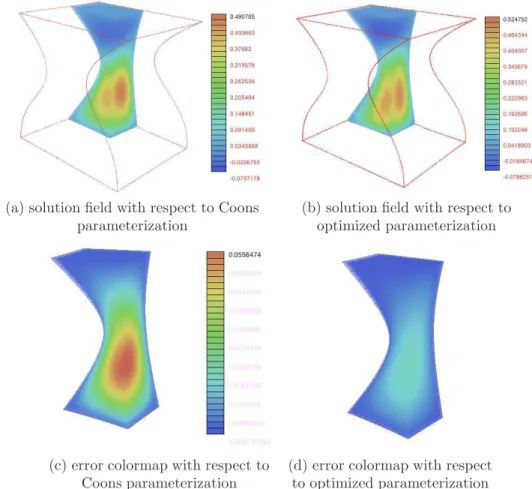
(a) solution field with respect to Coons parameterization
(b) solution field with respect to optimized parameterization
(c) error colormap with respect to Coons parameterization
(d) error colormap with respect to optimized parameterization
Fig.5. Simulation example of non-linear constraint optimization method. The colormap in (d) has the same scale as (c).
solver for 3D heat conduction problem (13) has been im-plemented as a plugin in the AXEL1 platform, yielding a B-spline volume as solution field. The proposed multi-block constraint optimization methods are implemented as a part of the isogeometric toolbox of the project EXCITING2.
In this paper, we test the different parameterizations of computational domains for the following heat conduction problem, ∇(κ(x)∇T (x)) = f (x) in Ω T (x) = T0(x) on ∂ΩD κ(x)∂T ∂n(x) = Φ0(x) on ∂ΩN, (13)
where x are the Cartesian coordinates, T represents the temperature field and κ the thermal conductivity. Dirichlet and Neumann boundary conditions are applied on ∂ΩDand ∂ΩN respectively, T0and Φ0 being the imposed tempera-ture and thermal flux (n unit vector normal to the bound-ary). f is a user-defined source function. In this paper, the source function is defined as
f(x, y, z) = −π 2 3 sin( πx 3 ) sin( πy 3 ) sin( πz 3 ). (14) The boundary condition is specified as T0(x ) = 0 and Φ0(x ) = 0.
1 http://axel.inria.fr/ 2
http://exciting-project.eu/
For problems with unknown exact solution T , suppose that This the approximation solution obtained by isogeo-metric method, then the discrete error e = T − Th. Hence, a posteriori error assessment can be obtained by resolving the following problem,
∆e = −f + ∆Th in Ω e = 0 on ∂ΩD
(15) The approximation error e from (15) also has a B-spline form. In order to achieve more accurate results for above problem, some h-refinement operation should be per-formed. Then we can obtain a good approximation of error volume. Though it is much more expensive, we can use it as an error assessment method to show the effectiveness of the proposed construction method of computational domain.
Fig. 5 (a) and 5 (b) presents the corresponding solution field obtained from the volume parameterization in Fig. 3 (c) and Fig. 3 (d) . The corresponding simulation error ob-tained from (15) are illustrated in Fig. 5 (c) and 5 (d) with same scale. The final parameterization obtained by the non-linear constraint optimization method can achieve better simulation results than the initial Coons parametrization, which illustrates that the optimized volume parameteriza-tion is analysis-suitable.
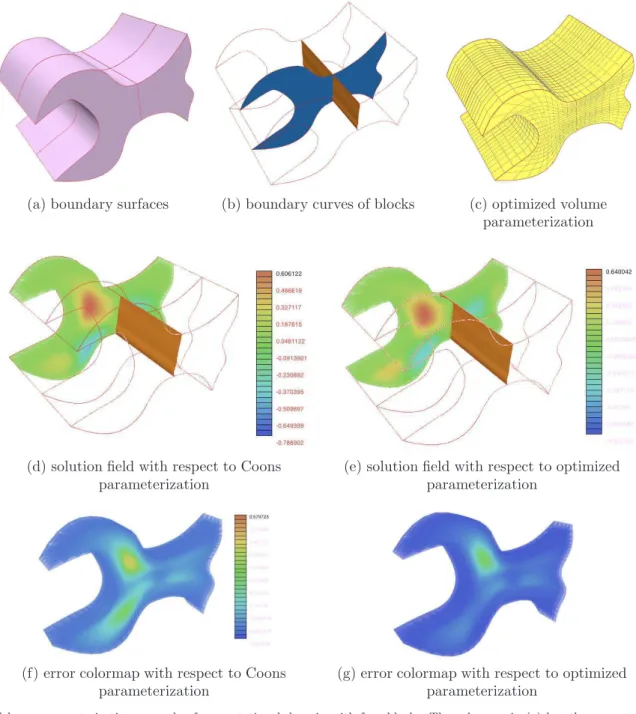
Fig. 6 presents a volume parameterization example with four blocks. The given boundary B-spline surfaces and
(a) boundary surfaces (b) boundary curves of blocks (c) optimized volume parameterization
(d) solution field with respect to Coons parameterization
(e) solution field with respect to optimized parameterization
(f) error colormap with respect to Coons parameterization
(g) error colormap with respect to optimized parameterization
Fig.6. Volume parameterization example of computational domain with four blocks. The colormap in (g) has the same scale as (f).
the block partition are shown in Fig. 6 (a) and 6 (b). Fig. 7 (c) shows the optimized volume parameterization of com-putational domain without self-intersections constructed by the non-linear constraint optimization method. Fig. 6 (d) and 6 (e) shows the corresponding solution field ob-tained from Coons parameterization and optimized param-eterization. The corresponding simulation error obtained from (15) are shown in Fig. 6 (f) and 6 (g) with same scale. In order to show the effectiveness of the analysis-suitable volume parameterization, the global cross sectional view of the computational results and error colormap are illus-trated. We can find that the optimized parameterization obtained by the non-linear constraint optimization method with C1 continuity constraints can achieve better
simula-tion results than the initial Coons parameterizasimula-tion. In or-der to show the C1continuity between two blocks, we pute the first derivatives at three sampling points for com-mon boundary surfaces between σ1and σ2and the common boundary surface between σ3and σ2, which are presented in Table.1.
Fig. 7 shows a volume parameterization example with five blocks. The given boundary spline surfaces and curves are shown in Fig. 7 (a) and 7 (b). Fig. 7 (c)(d) present the optimized volume parameterization of computational do-main without self-intersections by the quadratic program-ming method. In order to illustrate the effectiveness of the proposed method, the global cross sectional view of the or-thogonality colormap is shown in Fig.7 (e).
(a) boundary surfaces (b) boundary curves
(c) optimized volume parameterization (d) interior view of optimized volume parameterization
(e) interior view of orthogonality colormap
Table 1
The first derivatives at sampling points on the common boundary surfaces in Fig. 6. ∂σ1 ∂ξ ∂σ2 ∂ξ ∂σ2 ∂η ∂σ3 ∂η (0,0.16,1) (0,0.16,1) (-2.21,1.58,0) (-2.21,1.58,0) (0,0,1.33) (0,0,1.33) (0.73,1.03,0) (0.73,1.03,0) (0,0.35,2.98) (0,0.35,2.98) (1.07,3.04,0) (1.07,3.04,0) Table 2
Quantitative data for volume parameterization in Fig.3, Fig.6 and Fig.7. # deg.: degree of B-spline parameterization; # con.: number of control points; KVI: knot vector information ; # iter.: number of optimization iterations; # CT.: computational time in seconds; # MVA: mean value of orthogonality metric cosα+cos β+cos γ
3 .
Example # Deg. # Con. KVI # Iter. # CT. # MVA. Fig.3 p= q = r = 3 125 [0,0,0,0,1,2,2,2,2] 5 2.52 0.2033 Fig.6 p= q = r = 3 512 [0,0,0,0,1,2,3,3,3,3] 9 4.13 0.2567 Fig.7 p= q = r = 2 320 [0,0,0,1,2,2,2] 8 3.35 0.1356
Quantitative data of volume parameterization method presented in Fig.3, Fig.6 and Fig.7 are summarized in Ta-ble.2.
6. Conclusion
Analysis-suitable volume parameterization of compu-tational domain plays an important role in isogeometric analysis as mesh generation in finite element analysis. In this paper, volume parameterization problem of multi-block computational domain in isogeometric applications is studied. This problem is solved in a constraint opti-mization framework , in which the constraint condition is the injectivity sufficient conditions of B-spline volume parametrization, and the optimization term is the mini-mization of quadratic energy functions related to the first and second derivatives of B-spline volume parameteriza-tion. The resulted volume parameterization has no self-intersections, and the isoparametric structure has good uniformity and orthogonality. Finally, the continuity con-dition between the neighbor B-spline volume are added into the constraint term to achieve a multi-block volume parameterization. Several examples are presented to show the effectiveness of the proposed method.
In the future, we will investigate the impact of bound-ary surfaces on the volume parameterization results. For a given CAD model, how to obtain an effective volume par-tition is also an interesting topic for isogeometric applica-tions.
Acknowledgements
The authors wish to thank all anonymous referees for their valuable comments and suggestions. The authors are supported by the 7th Framework Program of the Eu-ropean Union, project SCP8-218536 “EXCITING”. The first author is partially supported by the National Na-ture Science Foundation of China (No.61004117), the Zhe-jiang Provincial Natural Science Foundation of China (Nos.
Y1090718), the Defense Industrial Technology Develop-ment Program(A3920110002), the Scientific Starting Foun-dation of Hangzhou Dianzi University(No. KYS055611029) and the Open Project Program of the State Key Lab of CAD&CG (A1105), Zhejiang University.
References
[1] M. Aigner, C. Heinrich, B. J¨uttler, E. Pilgerstorfer, B. Simeon and A.-V. Vuong. Swept volume parametrization for isogeometric analysis. In E. Hancock and R. Martin (eds.), The Mathematics of Surfaces (MoS XIII 2009), LNCS vol. 5654(2009), Springer, 19-44.
[2] K.H. Brakhage and Ph. Lamby. Application of B-spline techniques to the modeling of airplane wings and numerical grid generation. Computer Aided Geometric Design, 25: 738-750, 2008.
[3] Y. Bazilevs, L. Beirao de Veiga, J.A. Cottrell, T.J.R. Hughes, and G. Sangalli. Isogeometric analysis: approximation, stability and error estimates for refined meshes. Mathematical Models and Methods in Applied Sciences, 6:1031-1090, 2006.
[4] Y. Bazilevs, V.M. Calo, J.A. Cottrell, J. Evans, T.J.R. Hughes, S. Lipton, M.A. Scott, and T.W. Sederberg. Isogeometric analysis using T-Splines. Computer Methods in Applied Mechanics and Engineering, 199(5-8): 229-263, 2010.
[5] G. Celniker and D. Gossard. Deformable curve and surface finite elements for free-form shape design. Computer Graphics (Procs of SIGGRAPH’91) 25(4): 257-266, 1991.
[6] Cottrell JA, Hughes TJR, Bazilevs Y (2009) Isogeometric Analysis: Toward Integration of CAD and FEA. John Wiley & Sons, Chichester
[7] E. Cohen, T. Martin, R.M. Kirby, T. Lyche and R.F. Riesenfeld, Analysis-aware Modeling: Understanding Quality Considerations in Modeling for Isogeometric Analysis. Computer Methods in Applied Mechanics and Engineering, 199(5-8): 334-356, 2010.
[8] J.A. Cottrell, T.J.R. Hughes, and A. Reali. Studies of refinement and continuity in isogeometric analysis. Computer Methods in Applied Mechanics and Engineering, 196:4160-4183, 2007. [9] M. D¨orfel, B. J¨uttler, and B. Simeon. Adaptive isogeometric
analysis by local h-refinement with T-splines. Computer Methods in Applied Mechanics and Engineering, 199(5-8): 264-275, 2010.
[10] R. Duvigneau. An introduction to isogeometric analysis with application to thermal conduction. INRIA Research Report RR-6957, June 2009
[11] G. Elber, Y. Kim, M. Kim. Volumetric boolean sum. Computer Aided Geometric Design, 29(7): 532-540, 2012.
[12] J.M. Escobara, J.M. Casc´onb, E. Rodr´ıgueza, R. Montenegro. A new approach to solid modeling with trivariate T-spline based on mesh optimization. Computer Methods in Applied Mechanics and Engineering, 200: 3210-3222, 2011.
[13] G. Farin. Curves and Surfaces for Computer Aided Geometric Design: A Practical Guide, 5th Edition. Morgan Kaufmann, San Mateo, CA, 2001.
[14] G. Farin and D. Hansford. Discrete coons patches. Computer Aided Geometric Design, 16(7):691-700, 1999.
[15] P. Gill, W. Murray, M Wright. Practical Optimization. Springer, 1981.
[16] T.J.R. Hughes, J.A. Cottrell, Y. Bazilevs. Isogeometric analysis: CAD, finite elements, NURBS, exact geometry, and mesh refinement. Computer Methods in Applied Mechanics and Engineering 194, 39-41: 4135-4195, 2005.
[17] Li X, Guo X, Wang H, He Y, Gu X, Qin H. Harmonic Volumetric Map- ping for Solid Modeling Applications. Proc. of ACM Solid and Physical Modeling Symposium 109-120, 2007, Association for Computing Machinery, Inc.
[18] T. Martin, E. Cohen, and R.M. Kirby. Volumetric parameterization and trivariate B-spline fitting using harmonic functions. Computer Aided Geometric Design, 26(6):648-664, 2009.
[19] K. M. Morken. Some identities for products and degree raising of splines. Constructive Approximation, 7: 195-208, 1991. [20] T. Nguyen, B. J¨uttler. Using approximate implicitization for
domain parameterization in isogeometric analysis. International Conference on Curves and Surfaces, Avignon, France, 2010. [21] N. Nguyen-Thanh, H. Nguyen-Xuan, S.P.A. Bordasd and
T. Rabczuk. Isogeometric analysis using polynomial splines over hierarchical T-meshes for two-dimensional elastic solids. Computer Methods in Applied Mechanics and Engineering, 2011, 21-22: 1892-1908
[22] N. Nguyen-Thanh, J. Kiendl, H. Nguyen-Xuan, R. W¨uchner, K.U. Bletzinger, Y. Bazilevs, T. Rabczuk. Rotation free isogeometric thin shell analysis using PHT-splines. Computer Methods in Applied Mechanics and Engineering, 2011, 47-48: 3410-3424
[23] M.A. Scott, X. Li, T.W. Sederberg, T.J.R. Hughes. Local refinement of analysis-suitable T-splines. Computer Methods in Applied Mechanics and Engineering, 2012, 213-216: 206-212 [24] P. Wang, J. Xu, J. Deng, F. Chen. Adaptive isogeometric
analysis using rational PHT-splines. Computer-Aided Design, 2011, 43(11): 1438-1448
[25] J. Xia, Y. He, X. Yin, S. Han, and X. Gu. Direct product volume parameterization using harmonic fields. Proceedings of IEEE International Conference on Shape Modeling and Applications (SMI ’10), 3-12, 2010.
[26] J. Xia, Y. He, S. Han, C.W. Fu, F. Luo, and X. Gu. Parameterization of star shaped volumes using Green’s functions. Proceedings of Geometric Modeling and Processing (GMP ’10), LNCS 6130, 219-235, 2010.
[27] G. Xu, B. Mourrain, R. Duvigneau, A. Galligo. Optimal analysis-aware parameterization of computational domain in 3D isogeometric analysis. Computer-Aided Design , 2012, to appear [28] G. Xu, B. Mourrain, R. Duvigneau, A. Galligo. Parameterization of computational domain in isogeometric analysis: methods and comparison. Computer Methods in Applied Mechanics and Engineering, 2011, 200(23-24): 2021-2031
[29] G. Xu, B. Mourrain, R. Duvigneau, A. Galligo. Variational Harmonic Method for Parameterization of Computational Domain in 2D Isogeometric Analysis. Proceedings of 12th Conference on Computer-Aided Design and Computer Graphics, 223-228, Jinan, China, 2011