(
1)
THE DEFORMATION OF LARGE TELESCOPE
MIRRORS AND OPTICAL QUALITY
by
James P. Weldon,
S.M., Management, Massachusetts Institute of Technology B.S., Business Administration, University of New Hampshire
Submitted to the Department of Physics in Partial Fulfillment of the Requirements for the Degree of
Master of Science in Physics
at the
MASSACHUSETTS IN4S1fTUTE OF TECHNOLOGYJUN 0 5
1996
LIBRARIESMassachusetts
Institute
June, 1996
of Technology
1ai00nM.
clamz, to
Mfidormare~rr~
r hi nat,
of Author -'ý V - I--Deparment 0. ' of Physics Date Certified by John Tonry Professor of Physics Thesis Supervisor Certified by Accepted by Wit Busza Professor of Physics Thesis Reader I George Koster Professor of Physics Chairman, Departmental CommitteeV.'
Jr.
(1987) (1978) Signature --- ~---~----t---~----~C--- .THE DEFORMATION OF LARGE TELESCOPE MIRRORS
AND OPTICAL QUALITY
by
James P. Weldon, Jr.
Submitted to the Department of Physics in Partial Fulfillment of the Requirements for the Degree of Master of Science in Physics
Abstract
The 2.4 meter primary mirror of the MDM/Hiltner Telescope is modeled using the finite element method and analyzed for structural deformations caused by gravity acting on the mirror and its primary support systems. The finite element data is applied in two separate optical codes in order to analyze the effects of mirror surface deformation on image quality.
A series of point loads is applied to the mirror, and the resulting structural and optical perturbations are measured in order to ascertain the relationship between applied forces and deformation of mirror optical quality.
Finally, an active optics support system is proposed for the primary mirror. The design includes a linear optimization routine that acts to minimize reflected wavefront distortions by adjusting pressures in the new axial supports. The results of the active system predict that it is possible to achieve a diffraction limited image with the MDM/Hiltner Telescope.
In preparation for the finite element and optical analysis, and the design of an active optics system, the thesis introduces the theory of bending of thin plates, the methods of finite element and optical analysis, and the astronomical optics and wavefront aberrations appropriate to this subject.
Thesis Supervisor: John L. Tonry Reader: Wit Busza
ACKNOWLEDGMENTS
First and foremost, I would like to thank Professor John Tonry for inviting me to join him in this project, for his supervision, guidance, and ongoing help. Professor Tonry's insight and skill are matched only by his patience, his willingness to instruct, and his love of astronomy.
I would like to extend a special thank you to Dr. Martinus Van Schoor of MIT's Department of Aeronautics and Astronautics. Dr. Van Schoor generously spent many hours teaching me the methods of engineering mechanics and finite element analysis, and provided me with the facilities to complete the structural and optimization research.
I would like to also thank Professor Wit Busza for our discussions and his advice.
I am especially grateful to Keith Doyle of Lincoln Laboratories. Keith exhibited unlimited generosity in helping to verify the accuracy of the finite element model, answer questions, and generally supply moral and technical support. Special thanks to Lorenzo Williams, also of Lincoln Laboratories, for introducing me to Keith and making available my access to the Laboratories.
I would also like to thank all the people who work with Dr. Van Schoor at the Space Engineering Research Center of MIT's Department of Aeronautics and Astronautics for their support. SERC Director Professor Edward F. Crawley, Dr. David Miller, and SERC Administrator Sharon Leah Brown were very generous in allowing me the use of their computers, and granting me unfettered access to faculty, staff and graduate students.
Finally, I would like to thank my parents, Mr. and Mrs. James P. Weldon, and my grandmother, Mrs. J.D. Cahill Sr., for their unending moral and financial support.
Table of Contents
Chapter 1 1.1 1.2 1.3 Introduction... ... 7Background & M otivation ... 8
M DM and the Old School... 1 2 Objectives and Approach... 1 3 C hapter 2 The Beam Equation ... ... 15
2.1 Linear Relation Between Stress and Strain... ... 16
2.1.1 Properties of Stress ... ... 16
2.1.2 Displacements and Displacement Functions...18
.1.3 Hooke's Law & The Extension of a Beam...23
2.2 Pure Bending of Beams...25
2.3 A "Technical Theory" of Bending ... 29
Chapter 3 The Plate Equation...36
3.1 Plate Equation From Stress-Strain Relations... ... 37
3.1.1 Thin Plate Stress-Strain Relations ... 37
3.1.2 The Plate Eqn From Equilibrium Conditions...39
3.2 Plate Equation for a Circular Plate ... 45
Chapter 4 Analytical Solutions ... 46
4.1 Analytical Solutions to the Beam Equation ... 47
4.1.1 Cantilever Beam with a Point Load... ... 47
4.1.2 Cantilever Beam With Uniform Load ... 4 8 4.1.3 Cantilever Beam, Distributed & Point Loads...49
4.1.4 Simply Supported Beam & Distributed Force ... 50
4.1.5 Simply Supported Beam W. Point Load...51.. 1
4.1.6 Simply Supported, Gravity & Point Load ... 53...5 3 4.2 Radial Plate Analytical Solutions... ... 54
4.3.1 Solution to a Plate Clamped at the Edges ... 55
4.3.2 Solution for a Simply Supported Plate... 57
Chapter 5 Finite Element Analysis ... ... 59
5.1 Conceptual Finite Element Analysis... ... 60
5.1.1 Introduction to The Finite Element Method ... 60
5.1.2 Explicit Plane Truss ... ... 62
5.1.3 Utility of Direct Physical Argument... ... 64
5.2 Energy M ethods ... ... ... 65
5.2.1 Energy M ethod Definitions ... 65
5.2.2 The Principle of Minimum Potential Energy...66
5.2.3 Developing the Total Potential Energy... 68
5.3 R ayleigh-R itz ... 70
5.4 Analytic and FEA Methods Compared... ... 73
5.4.1 Cantilever Beam Numerics... ... 73
5.4.2 Simply-Supported Beam Numerics ... ... 76
Chapter 6 Introduction to Astronomical Optics... 81
6.1 Geometrical Optics and Image Formation... 82
6.1.1 How MDM Forms an Image... 82
6.1.2 Conic Sections of Revolution ... 85
6.1.3 Focal Length and Radius of Curvature ... 87
6.2 Physical Optics & Diffraction ... ... 90
6.2.1 The Diffraction Integral ... 91
6.2.2 Diffraction Limit & Point Spread Function...95
Chapter 7 Basic Aberration Theory... 98
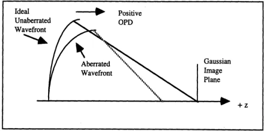
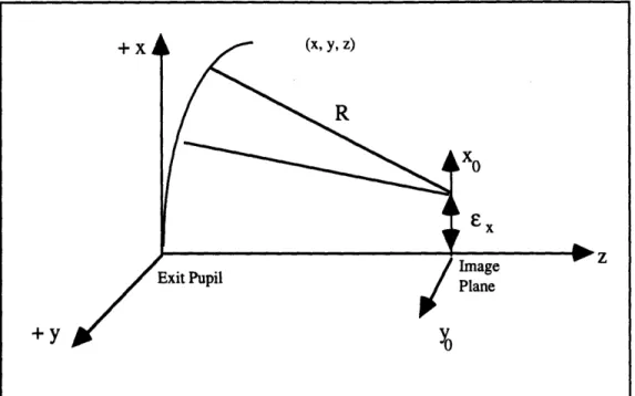
7.1 The Aberration-Free Wavefront... ... 99
7.2 OPD, Defocus and Lateral Shift ... ... 100
7.2 .1 D efocus... ... 10 1 7.2.2 Lateral Shift and Tilt... 102
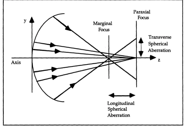
7.3 Angular, Transverse, Longitudinal Aberrations ... 104
7.4 Seidel A berrations ... ... 106 7.4.1 Spherical Aberration...108 7.4.2 C om a ... ... 110 7.4 .3 A stigm atism ... I 11 7.4.4 Distortion... 114 7.4.5 Field Curvature... 114 Chapter 8 8.1 8.2 8.3 Optical Analysis and Zernike Polynomials... 15
Zernike Polynomials and W avefront Fitting... 16
Table of Zernike Polynomials ... 20
PCFRINGE ... 122
Chapter 9 The Mirror, the Model & Model Verification... 23
9.1 The MDM/Hiltner Primary Mirror,... ... 124
9.2 FEA Model Description ... ... 127
9.2.1 Model Objectives...127
9.2.2 M odel A ssum ptions ... ... 128
9.2.3 Building The Basic Mesh ... 29
9.2.4 FE Model of the Axial Support System... 132
9.2.5 Modeling the Radial Support System ... 133
9.3 M odel Verification... ... ... 135
Chapter 10 Structural and Optical Analysis of MDM ... 141
10.1 Analysis of the MDM Primary Mirror ... .... 142
10.1.1 Mirror Structural Response ... .... 142
10.1.2 Optical Results For the Nominal Mirror ... 1...47
10.2 Mirror Resting on Hard Points ... ... 152
10.3 Single Point Load Perturbations... ... 158
10.3.1 Structural Response to A Point Load... 158
10.3.2 Optical Response to A Point Load ... 165
10.4 Perturbations From Two Point Loads ... .... 172
1.0.4.1 Structural Response, Pair of Point Loads ... 172
10.4.2 Optical Response, Pair of Point Loads ... 180
10.5 Perturbations From Two Pair ... 87
10.5.1 Structural Response , Four Point Loads ... 188
Chapter 11 Active Optics ... 202
11.1 Active Optics System Theory... ... 203
11.2 Description of the Active Optics System ... 206
11.3 Explanation of Design Configuration ... 12
11.4 Nominal Mirror Active Control... 13
11.4.1 Active Control of Perturbed Mirror...13
11.4.2 O ptical Results ... ... 218
11.5 Correcting Gravity and Point Load... ... 221
11.5.1 Active Control of Perturbed Mirror... 221
11.5.2 Optical Results of Active Control...226
11.6 Active Control of 100 Pound Point Load... ...229
11.6.1 The 100 Pound Perturbation ... 229
11.6.2 Optical Results, 100 Pound Point Load... 234
11.7 Correcting Perturbations From Gravity... .... 238
11.7.1 Active Control of Four 20 lb. Point Loads ... 238
11.7.2 Optical Results of Active Control...243
11.8 Correcting Two Pair of 100 lb. Loads ... .... 247
11.8.1 Active Control of Four 100 lb. Point Loads ... 247
11.8.2 Optical Results of Active Control... 251
Chapter 12 Conclusions and Recommendations ... 254
References ... 257
Chapter 1
Introduction
The goals of this thesis are to accurately model the primary mirror of the Michigan, Dartmouth, MIT 2.4 meter Hiltner Telescope (MDM), to produce a detailed structural and optical analysis of the mirror's performance, and to re-design the primary mirror's axial support system in order to minimize optical aberrations caused by gravity induced mirror deformation.
Two preliminary goals will serve to prepare for the finite element and optical analysis and axial support re-design. The first preliminary goal is to investigate the mechanics that explains the how the mirror responds to applied force. This is done by deriving the equations that describe bending of beams and plates, and applying those equations to analytical examples that share some commonalty with the MDM mirror.
The second preliminary goal is to describe the behavior of light as it enters and travels through a reflecting telescope. Of particular interest are
the nature of wavefront aberrations, the wave equations that describe these aberrations, and the specific optical testing methods that have been selected to quantify the aberrations in the MDM model.
1.1
Background & Motivation
The ability to collect light and to resolve images are the two primary performance criteria for a telescope. Aperture size determines a telescope's ability to collect light and contributes to the telescope's ability to see very faint objects. The other primary criteria, image resolution, is a measure of a telescope's ability to resolve small objects, or to resolve small, far away objects that lie in close proximity to one another. Resolution is a function of light collection ability, the quality of the incoming wavefront, and the quality of
the telescope's optics.
Anything that detracts from a perfectly formed image constitutes a problem for astronomers and for telescope designers. - Historically, the two
most persistent sources of imaging problems have been atmospheric turbulence and telescope mechanics.
Atmospheric turbulence is associated with temperature variations that cause changes in air density. These density changes cause some parts of an incoming astronomical wavefront to be slowed relative to other parts. The result is a spatial and temporal wavefront perturbation that can be defined as a complex phase aberration. The real part of the complex phase aberration is a phase shift of the wavefront - this is called "the seeing". The imaginary part of the phase aberration is a measure of intensity fluctuations known to astronomers as scintillation. Poets call it the "twinkling" of the stars.
Imperfect telescope optics are another major cause of blurred images. A perfectly formed incoming wavefront (no atmospheric turbulence or any
other sort of interference) that. reflects from a telescope's primary mirror will form a less than optimal image if any part of the reflecting surface suffers from deformation. Deformations typically are caused by gravity acting on the mirror's mass, externally induced vibrations that affect telescope structure, or temperature variations acting across the mirror. The result is that the mirror structure bends or deforms, and the optical surface loses its shape.
Until very recently, designers and astronomers have been limited in their attempts to correct the effects of either the atmospheric turbulence or
the telescope structure problems. Though the physics of turbulence has long been well understood, the technology for correcting a turbulence-degraded wavefront did not exist. And for a very long time, the best answer to gravity, thermal and wind induced distortions in the optical surfaces was to build a very rigid optic.
Overview of Telescope
Technology
Evolution
The very first telescopes were relatively primitive refracting instruments of small light gathering and limited resolving capability. The pace of early post-Galileo telescope development was limited by the difficulties encountered grinding and polishing large surface area lens. Another challenge was the requirement to properly suspend . the optic within the telescope tube so that the optical axis was properly aligned, and in such a way that the optic did not deform.
A major early innovation that addressed the problems of light gathering ability and optical and tubular support was the reflecting telescope. Isaac Newton, Guillaume Cassegrain and James Gregory in the early 17th century independently designed compact, reflecting telescopes that utilized secondary mirrors to redirect the reflected wavefront to a position acceptable for observing. Newton (using a folding flat mirror) , Cassegrain (using a small convex mirror), and Gregory (using a small concave secondary) defined the basic configurations of the reflecting telescope only fifty years after Galileo's first refractor.
For several centuries following the Newton era refracting and reflecting telescope designs competed with each other for astronomical primacy. Technology development followed an irregular path. While advances helped both designs, the early years favored the refractors. Innovations included advances in grinding, polishing and manufacturing lenses, the development of counterweights to improve tube suspension, and a discovery that some astronomical objects show a well defined, measurable parallax, which contributed a strong boost to the refractor's ability to render precise measurements. Refractors continued to be the telescope of choice through the end of the 19th century.
The optic suspension handicap proved to be an acute and persistent problem for the refractor community. Engineers could not support massive lenses while adequately maintaining lens figure and optical quality. This inability placed an upper bound on lens mass and aperture size. The Yerkes Observatory 40" refractor and the Lick 36" refracting telescope of the late
19th century represented the pinnacle of refracting technology.
A breakthrough innovation in the late 19th century was the development of the ability to deposit silver on glass. This made possible the manufacture of large area, precisely figured astronomical mirrors. The high quality of the reflecting surface made with the silver deposition technology gave reflectors optical and structural advantage over refractors. This advantage, combined with the problems inherent in . peripherally supported massive glass lenses, effectively made the refractor obsolete. The reflector became the instrument of choice.
The reflecting telescope breakthrough did not address the problems of telescope-optic support. As the primary mirrors grew very large, so did the challenges of building support systems that could maintain the mirror's designed optical figure. Increases in mirror size came at the price of increased weight, unwanted mirror flexure and the associated loss of optical figure and resolution. The traditional answer to the unwanted bending of the mirror brought on by the mirror's own mass and the action of gravity was to make very rigid mirrors. The thinking was that a stiff mirror made out of a material with a very low coefficient of thermal expansion would act, due to its own stiffness, to resist structural deformation.
Active and Adaptive Optics
This thinking began to change as early as 1953 with an idea by Horace W. Babcock, who proposed that a mirror's surface could be adapted in order to correct for errors in the phase of the incoming wavefront. Though Babcock lacked the resources to develop his idea, his bold vision initiated the innovations that would address not only the mechanical difficulties of astronomical optics, but the atmospheric difficulties as well.
The Strategic Defense Initiative, the 1980's era anti-missile effort of the US Department of Defense, adopted and developed Babcock's idea in order to develop a capability to optically identify Soviet satellites from ground-based sites. The SDI's success with deformable optics, now called active and adaptive optics, became available to civilian astronomical applications in the 1980's.
Active optics is a method for correcting the structural deformations commonly found in large astronomical mirrors due to the effects of gravity and thermal forces acting on the mirror's structure. The system bends the mirror back into shape and restores the required optical figure to the reflecting surface.
The active optics concept utilizes a deformable mirror, a set of actuators, and an information set. The actuators mounted on the back side of the mirror replace the traditional passive axial support system found in older telescope designs. The information set describes the mirror's known response to force inputs, as well as the differences between the mirror's optimal surface figure and the figure that actually exists as a result of mirror orientation and ambient conditions. This data is used in the actuator control system to adjust the mirror surface and correct structural deformations.
Adaptive optics is a much more ambitious technology. The adaptive concept is to rapidly alter the mirror surface by using a closed loop control system to compensate for phase changes in the incident wavefront caused by atmospheric turbulence. Adaptive optics systems include segmented, highly deformable thin mirrors, actuators and actuator control systems, wavefront sensors and data processors.
An adaptive optics system measures the relative phases of the components of the incident wavefront. This is done by segmenting the mirror surface, and measuring wavefront tilt in each zone. This information is fed to a control system which is responsible for positioning the actuators that drive each of the mirror segments. Given wavefront data, the control system adjusts the individual segments of the mirror's surface in such a way that any wave component arriving later than another actually travels a shorter distance to the focal point. A collateral benefit of adaptive optics is that the technology
inherently compensates for any mirror deformation problems that arise due to gravity, thermal forces or vibration.
The differences between the two types of systems is best seen by looking at their respective speeds. Few active systems work faster than 1 Hz - the mechanical causes of mirror system deformation addressed by active optics, gravity and heat, proceed on a relatively long time scale. Adaptive optics, on the other hand, compensates for rapidly varying atmospheric wavefront distortions. Some adaptive systems use bandwidths of 100 to 1000 Hz.
1.2 MDM and the Old School
The MDM /Hiltner Telescope located at Kitt Peak, Arizona is a member of the older school of reflecting telescopes. In the hierarchy of telescope evolution, MDM falls into the stage that just predates the onset of active/adaptive optics. The primary mirror, not considered deformable, is designed to rely on its own stiffness and support system in order to maintain correct optical figure.
The MDM primary mirror is 2.4 meters in diameter, and weighs approximately 1990 kg. The mirror is made of Cervit, a glass-composite material that is very stiff (Elasticity - 9.2 E10 N/m2) and that exhibits a very low coefficient of thermal expansion (approximately zero). The mirror rests in a mirror cell, supported by an axial and a radial support system.
Primary axial support is provided by a set of three neoprene air bladders. The air bladders are controlled to provide a constant pressure across the mirror's back surface. Also providing axial support is a set of three hard points located at radius = .825 meters, at intervals of 1200. The neoprene air bladders are adjusted by a control system so that the hard points support a load of no more than 30 pounds ( = 135 Newtons) in the axial direction. The hard points effectively constrain the mirror from moving in the radial plane. The pressure control that maintains a constant and uniform set of reaction forces on the hard points is the only active control component. Hence, MDM might be called a semi-passive, or tilt-active control system.
Radial support is provided by a neoprene mercury belt located along the mirror periphery at the axial center of mass. The mercury inside the belt acts an analog computer, feeding down to provide support as the mirror is rotated away from the zenith, or pure vertical orientation. The belt acts as a buffer between the mirror and the mirror cell. If the mirror is rotated to the horizontal, the mercury belt is sufficient to support all the mirror's mass.
The MDM/Hiltner telescope exhibits many of the problems common to heavy, rigid mirrors. Most of these problems are directly related to the mirror's mass, its primary axial support, and the lack of active control over the primary mirror's surface. This thesis endeavors to solve these problems.
1.3
Objectives and Approach
The principal objectives of this research are academic. If MIT continues its association with the MDM consortium, it is possible that the axial support re-design developed in this thesis will be implemented. Otherwise, it is hoped that the analysis contained in this study will help to improve the quality of information delivered by MDM/Hiltner. Academic objectives are as follows:
(1) Develop an accurate model of the MDM primary mirror and its support system to determine the nature of the structural and optical distortions that are induced by the action of gravity.
(2) Determine the mirror's reaction to force inputs, and develop a correlation between the mirror's reaction to force (Newtons) and its optical performance.
(3) Design a new axial support system that minimizes gravity induced deformations. Investigate the feasibility of an active axial support system.
Finite element analysis is the primary structural analysis tool. An optical analysis package that utilizes the method of Zernike polynomials, and a spot-diagram/contour-diagram code written by Professor John Tonry (MIT,
1995) serve as the optical analysis tools. The axial support redesign was accomplished with the aid of a least squares optimization code written by Dr. Martinus Van Schoor (MIT, 1995). The thesis is composed of three parts:
Part 1: Chapters 2, 3 , 4 and 5.
Chapters 2 and 3 investigate the mechanics of the bending of plates and beams and serve as a theoretical guideline for investigating the methods of structural analysis and finite elements. Chapter 4 is an exercise in fitting numbers to bending theory. Deflection solutions are found for a series of beams and plates under various load and support conditions. Chapter 5 introduces the method of finite element analysis.
Part 2: Chapters 6, 7 and 8.
Chapter 6 is a limited investigation of geometric and physical optics. Ideal wavefront behavior in a telescope system is discussed. Chapter 7 develops basic optical aberration theory. Chapter 8 describes the method of Zernike polynomials in optical analysis. Zernike polynomials are a set of orthogonal polynomials that act to decompose an aberrant wavefront. The individual polynomial coefficients are used to evaluate the relationship between measured optical surface distortions and active support changes.
Part 3: Chapter 9, 10 , 11 and 12.
Chapter 9 describes the finite element model of the MDM 2.4 meter mirror and support system. The model is verified by a real world experiment done at Kitt Peak. With the telescope in a purely vertical orientation, a telescope technician drained the air from the axial air bladders, which put the mirror to rest on the three hard points. A star image was taken. The same procedure was accomplished with the model, and the optical results are compared to the actual results.
Chapter 10 presents the results of finite element and optical analysis for the mirror under various load conditions. Both finite element and optical data are presented. Chapter 11 proposes and tests a new active axial support design based on unit load response and a least squares optimization. Chapter 12 offers lessons learned and recommendations.
Chapter 2
The Beam Equation
This chapter introduces the mechanics of bending of rigid bodies and develops an equation that describes bending in solid beams. This derivation follows the presentation of classic mechanics in Housner (Ref. 1) and Timoshenko (Ref. 2). In combination with the next chapter's treatment of the plate equation, this chapter will serve as a prelude to the analytical and numerical study of the mechanical behavior of the MDM/Hiltner Telescope's 2.4 meter primary mirror.
Linear stress-strain relations, displacement functions and Hooke's Law form the basis for both the theory of elasticity and the beam equation. The beam equation,
d4v
EIx~ = P.
describes a solid beam's response to applied force. The equation assumes a linear stress-strain relations to calculate the deformation of a solid body under the influence of stress.
2.1 Linear Relation Between Stress and Strain
A linear stress-strain relationship means that a solid body (a wooden
beam or a telescope mirror) will deform in proportion to the applied force. These changes in geometry can be predicted with a high degree of accuracy if the applied stress is within that material's elastic limits. When stressed beyond elastic limits, the material becomes plastic and will not recover its shape.
2.1.1
Properties of Stress
Stress is defined as force per unit area:stress = lim force A -0 area
The stress vector has two components, the normal stress vector and the tangential stress vector, as shown in Figure 2.1. The normal stress vector is denoted by the symbol 6, and is defined as the force per unit area that acts normally to the face of a solid. The three components of normal stress are ax,
Ty, and oz, such that Cx is a stress normal to the x-face on which it is acting.
The stress that acts tangentially to the face of the solid is called the shear stress. Shear stress is denoted by t; txy means that I acts on the x-face in a direction parallel to the y-axis.
Figure 2.1: Total stress vector is a combination of normal and shear stress.
A complete description of the state of stress of a body requires that the stress at every infinitesimal point in the body be known. For any given point in a body, the total stress is a linear sum of normal and tangential stress.
stress = a~ x + Tx•y + rxz
stress, = T + a y + y,,z (2.1)
stress = tZx + zyY + (7z .
From equations (2.1), the state of stress experienced by a body at any point can be represented by a matrix of nine scalar stress components:
T C
'r
Yr
Z x ly xTz yx Zy yz,Zr·
auZ
U, ZY z = stress.For a small body element to be in static equilibrium, the vector sum of all forces acting on that element must be zero. Equilibrium also requires that the sum of all moments be zero. In the case of a three dimensional solid element, the stress tyyx multiplied by the area on which it works equals a force T yx dx dz. This force multiplied by a radius dy gives a moment 'Tyx dx dy dz. Equilibrium requires that the sum of the moments be zero, therefore
"yx dx dy dz = Txy dx dy dz.
Since the areas are equal, in an equilibrium state opposing shear stresses are equal and indistinguishable:
Txy =
Tyx
,and for any element in equilibrium, the two in-plane components of shear stress are equal.
2.1.2 Displacements and Displacement Functions
The deformation of a solid body can be described in terms of displacements of any point within that body. For a continuous body that exhibits a linear response to stress, these displacements are functions of position. The displacement functions u(x, y, z), v(x, y, z) and z(x, y, z) describe the displacement of a small element of a continuous body under stress from some original position P(x, y, z) to a new position P'(x, y, z).
For a body to be considered continuous, all physical properties must be specified at every point and be continuous throughout the body. This definition effectively states that the average properties of a small element of a material may be used to characterize the entire material's volume.
Displacement of a point within a continuous body may result from rotation, deformation, or translation. (This paper will not address translation.)
Rotation
Figure 1.2 shows the rotation of a small unit element about a point. This rotation produces displacements that can be defined in terms of position. In the figure, a small angle rigid body rotation occurs at a point "A" about the z-axis. The rotation "wz" of the square element displaces corner "B" .
X
Figure 2.2: A small body rotation about a point "A".
m
cody
z
The displacement relative to "A" due solely to rotation are
(du)rotation = COy dz - COz dy (dv)rotation = (Oz dx - COx dz (dw)rotation = Oxdy - Cty dx.
The components of rotation can be generalized (eqn (2.3) below):
1 dw
dv
S2
(dy
dz)
Normal Strain
Normal strain of an element is defined as an incremental change in the element's length divided by the element's original length. Extension is positive strain, while contraction is negative strain. Figure 2.3 (below) shows positive strains experienced by a small element as the result of normal stress.
x
4-) = 8 dx
x
Y4
Figure 2.3: An element showing normal strain. Each side has of the element has been extended a small fraction of its original length. Positive strains shown in Figure 2.3 are defined by "e":
A (dy)
A (dz)
' dy e dz (2.2) A (d A(dy) = E dyA
(dx)
dx (2.4)1 dud
dw
tx =2 (Id~z
dx
l
=(u
x2dz dx
dw
Figure 2.4. (below) shows the positive strains of the element in terms of displacements. The x and y coordinates of the corners of the element have been displaced in the x- and y-directions as a result of a stretching of the material in the element.
Figure 2.4: Positive strains in terms of displacement functions.
The element has been stretched in the x-direction by an amount
(du) normal strain = A (dx) =x + dx + u + dx - (x + dx + u).
The x-, y-, and z-direction displacements are found by canceling terms:
(du),, normal strain =A (dx) = - dx.
dx
(dv) normal strain = A (dy) = -dy,
dw
(dw) normal strain A (dz) = -dz.
dz
Normal strains (from eqn 2.4) are defined in terms of displacements by
du
dv
dw
dx' 8 dy ' Zd(2.5)
(2.6) + ayx dx, y+v )I
(x+u, y +dy+v+ d ady)
F
Shearing Strain
An element can deform without changing the length of its sides. In this "shear strain" case, called distortion or pure shear, neither rigid body displacement, normal strain nor rotation are involved. The element experiences a change in its geometry that is best characterized as an angular deformation, as shown in Figure 2.5:
x
Y
Figure 2.5: Shearing strain as two simple shearing deformations.
The total shearing strain in Figure 2.5 is 7xy = xy + Eyx
where the terms Exy and Eyx describe angular deformations of the sides "dx"
and "dy" and are called the xy-components of shearing strain of the element. If there is no rotation involved in the displacements, e = e y
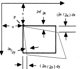
The shearing strains can be expressed in terms of displacements. As can be seen in the Figure 2.6, the rate of change of displacement with respect to the x- and y-axis define the total shearing strain.
uy
ay
Figure 2.6: Shear strain as rates of change of displacement functions.
Shearing strains are defined in terms of displacements:
dv
du
xy dxdy
'y =Z - + -
dv
dz d
dw
Y'x =
du
dz
+x
Tx
dw
Summary
The state of strain at any point in a continuous body can be specified by examining the variations in displacements. Displacements are functions of position and result from rotation, normal strain and shearing strain. The total differential of the displacement functions is:
du du du
du =
-dx
+-dy +-dz
ax
dy
dz
dv dv dvdv = -dx + -dy + dz
dx
dy
dz
dw dw dwdw • dx + -dy + dz.
dx
dy
dz
(2.8) (2.7) av av /Bx) dx - ( Du / ay) dy2.1.3
Hooke's Law & The Extension of a Beam
Hooke's Law states that a solid material will deform in proportion to the applied force. Hooke formalizes the linear relationship that exists between stress and strain in many materials. Strains from normal x-axis stress are
1
ex - x, E V y = -E xx , V E (2.9)Figure 2.7 illustrates the meaning of the constants E and "v". The elasticity "E" is defined as the ratio of longitudinal stress/strain, E= / .. The ratio of contractive strains
Poisson ratio
Y and 8 z to the tensile strain Ex is the
(ratio of contraction in y and z for stretching in x ).
Figure 2.7: Normal stress acting on a beam element showing contraction in y and z for stretching in x.
Equations analogous to equation (2.9) define a body's response (strain) to force (stress) applied in the y and z directions.
v 1 v
For a z-direction linear the force, the stress-strain relations are
V x -- z, V Y = -- O Y &E
1
z E(2.10)
(2.11) mThe linear relation between shearing stress and shearing strain is
xyG 7 =G
where the term "G" is the shearing modulus. The complete description of linear deformation includes terms for thermal expansion, normal and shearing stress. For an isotropic material, Hooke's Law is:
x E(ax-
v
- z ) xy GE nG E
EB
G
Beam
Extension
Figure 2.7 shows a solid beam of known material under direction stress. If all other stresses equal to zero:
a constant
x-x = o y z Txy xt Tyz.
(2.13)
The resulting linear strains are
1 Ex Co E v y 0-E E
There is zero shearing stress:
V
ez -= =o.
E
7 xz = 7 xy = yz = 0
The length of the beam increases by an amount proportional to the force, if it remains within the elastic limits of the material. The measured increase in length is ALX = L = aL sL E E F = (rx)(Area), , (2.14) (2.15)
2.2
Pure Bending of Beams
A beam bends in reaction to an applied load. The load may be due to gravity or to a point loading somewhere along the beam's length. Consider a cantilever beam that experiences a vertical force at its free end. Assume that the applied load, represented by a delta function, bends the beam slightly, but not enough to induce any shearing strain.
The beam experiences both compression and tension as it bends. For a downward force (please see Figure 2.8) the material at the top of the beam along the long axis will be pulled slightly apart, while the material along the bottom of the beam will be compressed. The crunching together of the lower part and the pulling apart of the top part are manifestations of horizontal stress induced by the action of the point load acting at the beam's end.
Figure 2.8: Cantilever beam with point load showing both compression and tension. The neutral axis runs between the top and bottom of the beam and experiences no strain.
If the applied force in Figure 2.8 is constant, the beam reaches a point of static equilibrium where sum of all forces acting on the beam equals zero:
+ e9y + F (gravity)= 0 (2.16a)
dx
dy
+ + Fy(gravity)=O0 (2.16b) Point Loadt
x
IFrom the diagram, ax is solely a function of "y", where "y" is a measure
of disyance from th neutral axis. The point load creates a smoothly varying horizontal stress that is a linear function of y-axis position:
x = y= cy. (2.17)
Yo
The total stress in the x-direction is the integral sum of the incremental stresses over the entire face of the beam. The total force experienced by the beam is the integral sum of linear stress multiplied by incremental area:
Fx = IrxdA =
JcydA,
and c1 = oYo
The linear stress described in equation (2.17) acts incrementally and at
a distance from the beam's neutral longitudinal axis giving rise to a bending
moment. Each stress increment acts at some small distance from the neutral axis, creating a little unit of torque. The total moment is the integral sum of these cross products. Since the applied stress is oriented in the x-direction and varies linearly with y, the moment acts about the z-axis in the y-direction:
Mxz = yoaxdA . (2.18)
The subscript "x" denotes the direction of the applied force, and the subscript z denotes the axis around which the beam bends. From the definition of the stress in equation (2.17), the moment equation can be expanded
Mx = fyx dA = Jcy2 dA = cIl (2.19)
where "I", the second moment of area, is defined
Iz = J y2 dA =
J y
2dxdy . (2.20)The stress can now be defined in terms of the bending moment, the second moment of area, and the radius from the neutral axis:
(2.21)
M
ax = cy= xzy
IZ
Hooke's Law thus relates stress to strain, and strain to bending moment,
I
ex
-E 1E
=
(2.22) El,Radius of Curvature and the Beam Equation.
Strain and bending moment are related to the beam's radius of curvature. The radius of curvature is defined by the displacement of the beam's neutral axis. This relationship establishes a differential equation for displacement which is known as the beam equation.
The angle between the undisplaced and the displaced neutral axis in Figure 2.8 is equivalent to tan 0 =dv/dx. For a very small angle, tan 0 is approximately equal to 0:
tan 0 = dv/dx 0 = tan 0 = dv/dx.
The radius of curvature of bending is defined as (Ref 3)
3
Rx = (dvoldx)j = a constant
d2
v/
dx2 (2.23)where Vo is a displacement in the y-direction. In the limit of small
deflections, (dvo/dx)2 approaches zero and the curvature can be defined as a second order condition of the deflection:
S= d2 V
/d 2.
Rx (2.24)
Arc length ds is defined: R dO = ds. Therefore, (dO / ds) =
1
= d2vo0/d 2.
The trick, at this point, is to relate the strain E x to the radius of curvature, and thereby derive a second order differential equation of bending. This is done in Housner (Ref. 4) by examining a beam element under horizontal (x-direction) stress that bends around the z-axis in the y-direction.
In the Housner relation, the neutral axis defines the coordinate system, so that "y" is a measure of vertical distance from the undisplaced neutral axis. The geometry of the beam element shows that the displaced beam's radius of curvature, the angle dO between the displaced and undisplaced neutral axis, the arc length ds of the element's displaced neutral axis, and the x-direction
strain are related by the equation
y dO = Ex ds.
From the above relation,
1/R = Ex/y
Therefore, the curvature is related to the second derivative of the deflection, and the moment:
1 M d2v
=- = (2.25)
R
EI
dx
This produces a second order equation for displacement and moment: d2v
EI = M (2.26)
dx2
Combining (2.25) and (2.26) establishes a second order equation which can be integrated to obtain a function for the y-axis displacement of the beam:
d
2vo
_d
=
.
(2.27)
dx2 ds Elz2.3
A "Technical Theory" of Bending
The methodology of "pure bending", described in Section 2.2 , requires an exact stress function. Since exact stress functions are rarely available, it is possible to construct approximate displacement functions by using equilibrium conditions as long as beam deflections remain small and the forces acting upon the beam cause little or no shearing strain. In the language of beam theory, the idea of small deflections translates to "plane sections remain plane", so that any cross section of the beam that is planar before bending will be planar after bending. Practically speaking, the criteria for applying this approximation technique is to use beams that experience little or no shearing stress and that exhibit a ratio of beam depth to length that is much less than one.
This section develops the "Technical Theory of Bending" for a beam of continuous and isotropic construction and symmetric cross section. The assumptions are summarized below:
E x
E
(2.28)
Y =0
(2.29)
Yx = 1 • = y z 0 (2.30)dv <<1.
(2.31)
dx
The first equation is Hooke's relation between stress and strain for materials operating within the limits of their elasticity. The second equation specifies that the beam experiences no y-direction strain. The deformation of the beam is limited to expansion and contraction in the x-direction. The third equation is the condition that there is no shearing strain. Lastly, the fourth equation explicitly limits beam deformation to small angles, thus completing a small scale, no shear, bending-only scenario.
Under the assumptions given, the y-direction strain is zero, so the displacement function v is solely a function of x:
v = f, (x).
Shearing strain is also zero,
du
dv
dy
ax
and the displacement u is a function of both x and y:
dv
u = -direction strain is given by
Since x-direction strain is given by
du
= , then x xd
2v
E, = -y-dx2 d2vand
T
= EE8 = -Eydx2
The bending moment is the integral sum of the applied force multiplied by the radius of action:
MXZ
= -f
ygdA = J Ey2
d
2-
(2.35)Since "dA" is equal to (dy dz), the integral is an expression for the moment of inertia of the cross-sectional area about the z-axis:
d2v
_d
d
2v
M, = E-
'y
2dA = EI
2 xzdX
2J dx2 d2vM = El
xt
ZdX2
(2.36)Equation (2.36) describes a beam experiencing small bending deflections.
(2.32)
(2.33)
The Beam Equation From the Applied Loads
The equations of equilibrium are of three types: forces parallel to the beam axis, forces normal to the beam axis, and moments. A differential relationship exists between the bending moment and the beam's equilibrium condition. The figures below depict a beam under a point load, and a free body diagram of a beam element.
X
Figure 2.9: A cantilever beam under a distributed load, showing x-direction stress and displacement function v(x,y).
+ dT
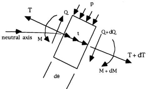
M + dM/
de
In Figures 2.9 and 2.10, "t" is a distributed force per unit length along the beam's neutral axis, "Q" is the shearing force, "T" is the tension resulting from x-direction stress, and "M": is the moment. Element length is "ds". Forces parallel to the axis and in equilibrium are:
dT
dO
tds + dT - QdO= , -- = -t +
Q
ds
ds
Forces in equilibrium normal to the beam axis are:
dO
dO
dQ + pds + Tsin
+ (T + dT) sin-• = 0.
2
2
Moments in equilibrium are:
(2.37)
(2.38)
dM + Qds = 0
The small angle approximation
dM
ds
sin
=
8,
drops the second order term:dQ
TdO
ds
ds
The second derivative of M can then be related to the derivative of Q:
d
2M
dQ
dO
ds
2ds
ds
The basic beam equation-moment identity (2.36 ) is substituted:
d2v MU=El xz d2
dM
d
2M
=
El
= p+T
Zdx2
d
2v
ds
ds2 Z dx" dx2ds
(2.39) (2.40) (2.41) (2.42)For a situation where T = 0, the equation is fourth order in terms of the applied load. The beam equation becomes
d
4v
Dimensional Analysis of the Beam Equation
A brief dimensional analysis of displacement functions and their derivatives will shed some light on the fourth order equation that describes action in terms of force per unit length. The displacement functions u(x,y) and v(x) are in units of length:
v(x) => meters.
The first derivative w.r.t. space is the slope, and is dimensionless:
dv
dx
The second derivative has units of inverse length. When multiplied by the elasticity and second moment of area, units of torque result:
d'v _ dO 1
d
2
d
-
(meters
'),
dx
2ds
N
_kg
Em
m2 s2m I = f y2dydzm
4d
2v
EI- = M dx 2N
41
m 2 mThe first derivative of the moment (which displacement function) is the shear force:
dM
dx
is the third derivative of the
kg m
s 2
Finally, the second derivative of the moment (which is the fourth derivative of the displacement) gives force per unit length:
d2M dQ 2 d2 N
dx2
dx
dX 2 mDelta Functions and Half-Range Functions
A likely place to apply the technical theory of bending is to a beam that experiences forces of known magnitude, position and direction, but whose exact stress distribution is unknown or is not continuous. These forces may be distributed along the length of the beam, or be concentrated in certain positions. An example of a distributed force is the body force generated by the beam's mass acted on by a gravity field. Examples of concentrated forces are end supports of a simply supported beam, or point loads that are applied at some position along the length of the beam.
The point load at the center of a simply supported beam represents not only a concentrated force, but a serious discontinuity problem. The solution to this potential conundrum is the "half-range" function, which is a member of the family to which Dirac delta functions belong.
One of the defining properties of delta functions that makes them so appropriate for this type of work is the fact that a delta function has value only at one spot. Everywhere else, it has zero magnitude.
45(x-a)=0 for x a
The other property of the delta function that makes it appropriate is that the delta spikes to infinity, but the area under the curve is equal to unity. It therefore acts as the perfect modifier to a point load of arbitrary magnitude:
+00
fI6(x)=1.
It is useful to view the delta function as a member of a set of functions called half-range functions. By definition, half-range functions produce a value only when the argument is positive:
{x-a} = 0
forall (x-a)
< 0,
The half-range functions are denoted by brackets. The delta function, considered as a member of the larger set of half-range functions, is defined as
3(a) = {x - a}- .
The general differential forms of the half range functions
d
__{x-dx
d
x-dx
a}" = n{x-a}'
"-a}' ={x-a}
0=0
for
for
=1
for
are :n•O
x<a x>ad
d{x -a
=
dx
{x -a}
-' = 0
for
=00for
x<a and x>a
x=a
=-{x - a}-2 = 0 for
=+oW
for
x<a and x>a
x = a
The half-range functions can be shown in integral form. integral of the delta function generates a step function.
{x-a}
"-0
1
dx
=
{x-a}"
n
for
Note that the
n
0.
j{x-a}-'dx= {x-a}.xf {x- a}° dx= {x- a}
1.
0 xf {x - a}'dx= {x-a}
2 0xI-)
d·I-)
f f x- alldx Ix- al
d
d{x - a}-'
dx
Chapter 3
The Plate Equation
This chapter derives the radial plate equation,
V'w(r) =q
D
Stress-strain relations, equilibrium equations and deformation conditions are used to develop the equation of bending of a thin plate which experiences a force perpendicular to the plate's horizontal plane. The motivation for this derivation is found in the classic mechanics texts written
by Timoskenko (Ref. 5) and Housner (Ref. 6).
The plate equation in conjunction with appropriate boundary conditions will be used to approximate the mechanical behavior of the MDM primary mirror and provide an analytical check for results obtained with the
3.1
Plate Equation From Stress-Strain Relations
This derivation of the plate equation uses the example of a thin, isotropic plate built of uniform material which experiences a relatively small vertical stress and zero vertical shear. The plate deforms in such a way as to produce no stretching or contraction of the middle surface.
These initial conditions allow deformation of the plate only by horizontal bending strain. This means that the middle axis or "neutral axis" of the plate will be displaced, but not deformed. This eliminates the possibility of middle surface z-direction strain. Any load that is applied to the plate will contribute zero shearing stress to the plate's middle surface.
3.1.1
Thin Plate Stress-Strain Relations
The thin plate shown in the diagram below exhibits a depth that is much less than its length or width. The plate's middle surface lies in the x-y plane. The depth is measured in "h" units. The top surface is located at coordinates (x, y, z = h/2), while the bottom surface is located at (x, y, z = -h/2).
I
I
I
I
Figure 3.1: A thin rectangular plate with middle surface in the x-y plane. The conditions described above are those that were used to justify the technical theory of bending of beams in Chapter 2. The technical theory of bending of a thin plate uses deformation and stress-strain conditions to develop a function w(x,y) that describes the transverse displacements of the middle surface of the plate. (Please see Table 3.1.)
Y
I
Table 3.1: Assumptions for technical theory of bending of a thin plate. Equation (3.1.a) states that "w" is independent of "z", so that the displacement of the middle surface is a function of only x and y. In other words, all points through the thickness of the plate that share the same x and y coordinates are displaced from their equilibrium positions relative to the
middle surface by the same amount. There is no pure z-direction strain.
Equations (3.1.b) and (3.1.c) state that there is zero middle surface shearing strain. Equations 3.1.d-f describe the x- and y- direction bending strain.
The displacement functions in the x, y and z-directions are:
dw du dw du
+-= 0 (3.2.a) +-= 0 (3.2.d)
du
dw
d
dw
d-
d
(3.2.b) _ = -- (3.2.d)dw
dw
u= -z + fl(x,y) (3.2.c) v=-z-+ f2(x,y) (3.2.e)
From Chapter 2, normal strain is defined as the rate of change of displacement with respect to position:
du = - (3.3) = . (3.4)
6= (3.3) . (3.4)
Substituting equations (3.3) and (3.4) into (3.2) yields a relation between normal strain and the displacement functions u(x,y) and v(x,y):
du d2w
Z
T
-2
Edv
- . (3.6)0 0ý
(3.5)
Horizontal shear stress deforms the plate through the angle y. Shear strain is the rate of change of "u" and "v" with respect to "y", and "x".
I du dv
S G- dy dx
Substituting equation (3.2.c) and (3.2.e) into (3.7) leads to a second derivative of "w" with respect to both x and y:
(3.7) du = 2w
q -dxdy
(3.10) dv d 2wx
=
-z
axdydx
The resulting strain-displacement relations between normal x- y- direction strain and the displacement function w(x,y) are:_u d2w
x d-
d-z
dv
2w
dy=
d=3.1.2
The Plate Equation From Equilibrium Conditions
The plate equation is derived by relating the strain-displacement conditions of equation (3.9) to the applied load. The trick is to isolate the z-direction normal stress as a function of middle surface displacement. Unfortunately, the z-direction normal stress appears in the equilibrium equations only in a relation with yz and T'. So there is some work to do.
The first step in deriving the fourth order plate equation is to list the general equilibrium equations for a plate under stress. The next step will be to invert the stress-strain relations in Table 3.1. The most tedious chore is to substitute the inverted stress-strain relations into the general equilibrium equations, and then determine by integration the shear and normal stresses.
(3.8)
and shear
2d 2w
The actual equation will result from equating the normal stresses to the intensity of the applied load at the upper surface of the plate.
Step 1: The General Equilibrium Equations
For a rigid body in equilibrium the sum of all forces and torques (moments) that act on the body must be zero:
SForces = 0
C
Moments = 0.The general equilibrium equations that describe the plate at rest are:
da x
-+ + -
d+
=O
&x dy dzda, drz
d%
L + + Yz + + = =00 + z + d = 0. ay az axStep 2: Invert the Stress-Strain
(eqns 3.10)
Relations
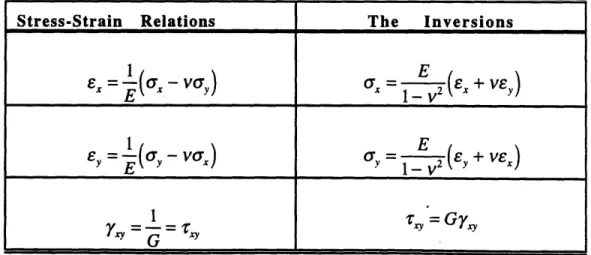
Inverting these relations expresses the plate's stresses in terms of strains, Poisson ratio, elasticity and shearing
Stress-Strain Relations The Inversions
1E
(a
=
.
)
E (Ex+ VEE E 1- v2 1E 1 = -I - va=) , = E +VEx y E 1- v 27x
=1
Y
rx
=Gyxy
GTable3.1: Inverted stress in a thin plate as a linear function of strain.