HAL Id: halshs-01278873
https://halshs.archives-ouvertes.fr/halshs-01278873
Preprint submitted on 25 Feb 2016
HAL is a multi-disciplinary open access
archive for the deposit and dissemination of sci-entific research documents, whether they are pub-lished or not. The documents may come from teaching and research institutions in France or abroad, or from public or private research centers.
L’archive ouverte pluridisciplinaire HAL, est destinée au dépôt et à la diffusion de documents scientifiques de niveau recherche, publiés ou non, émanant des établissements d’enseignement et de recherche français ou étrangers, des laboratoires publics ou privés.
Spillovers Matter?
Eric Nazindigouba Kere, Somlanaré Romuald Kinda
To cite this version:
Eric Nazindigouba Kere, Somlanaré Romuald Kinda. Climate Change and Food Security: Do Spatial Spillovers Matter?. 2016. �halshs-01278873�
C E N T R E D'E T U D E S E T D E R E C H E R C H E S S U R L E D E V E L O P P E M E N T I N T E R N A T I O N A L
SÉRIE ÉTUDES ET DOCUMENTS
Climate Change and Food Security: Do Spatial Spillovers
Matter?
Éric N. Kéré
Romuald S. Kinda
Études et Documents n° 4
February 2016
To cite this document:
Kéré E. N., Kinda R. S. (2016) “Climate Change and Food Security: Do Spatial Spillovers Matter?”, Études et Documents, n° 4 , CERDI.
http://cerdi.org/production/show/id/1788/type_production_id/1
CERDI
65 BD. F. MITTERRAND
63000 CLERMONT FERRAND – FRANCE
TEL.+33473177400
FAX +33473177428
2
The authors
Éric N. Kéré
PhD in Economics, Postdoctoral research fellow, CERDI – Clermont Université, Université d’Auvergne, UMR CNRS 6587, 63009 Clermont-Ferrand, France.
E-mail: [email protected]
Romuald S. Kinda
Assistant Professor, Université Ouaga 2,UFR-SEG 03, BP 7210, Ouagadougou 03, Burkina Faso.
E-mail: [email protected]
Corresponding author: Eric N. Kéré
This work was supported by the LABEX IDGM+ (ANR-10-LABX-14-01) within the program “Investissements d’Avenir” operated by the French National Research Agency (ANR).
Études et Documents are available online at: http://www.cerdi.org/ed
Director of Publication: Vianney Dequiedt Editor: Catherine Araujo Bonjean
Publisher: Mariannick Cornec ISSN: 2114 - 7957
Disclaimer:
Études et Documents is a working papers series. Working Papers are not refereed,
they constitute research in progress. Responsibility for the contents and opinions expressed in the working papers rests solely with the authors. Comments and suggestions are welcome and should be addressed to the authors.
3
Abstract
This article analyzes the role of spatial spillovers in the relationship between climate change and food security in developing countries over the period of 1971-2010. Using a Samuelson’s spatial price equilibrium model (theoretically) and Spatial Durbin Model (empirically), results show a strategic substitutability between the levels of food availability in the countries suggesting that an increase of food availability in a given country decreases the food availability of neighboring countries. Second climate change (water balance variability, droughts, floods and extreme temperatures) reduces food availability both in the affected countries and its main food trading partners. Third, food demand factors in a country may have the opposite (asymmetric) effect on its major trading partners. Fourth, supply factors have symmetric impact on food availability.
Keywords
Food security; Climate change; Spatial spillovers; Spatial econometrics; Developing countries.
JEL Codes
C23, Q17, Q18, Q54
Acknowledgements
4
1. Introduction
Over the last two decades, the number of people affected by extreme poverty has decreased from 1.9 billion in 1990 to 836 million in 2015 and the percentage of undernourished people has dropped by almost half from 23.3 per cent to 12.9 per cent. In 2015, the United Nations launched the Sustainable Development Goals (SDGs) initiative that aims to end poverty and hunger by 2030. Addressing issues related to food security is included in year fifteen of the development agenda. According to The
State of Food Insecurity in the World report (SOFI, 2015), 795 million people were
undernourished in 2015. Although hunger has been reduced in developing countries, progress has been hindered by several factors including political instability, less inclusive economic growth and climate events (St.Clair & Lynch 2010).
The economic literature on the impact of climate change on food security and production can be divided into two strands. In one body of literature, several authors develop theoretical arguments or prospective studies which indicate that climatic variability has a negative impact on agricultural production and decreases food availability. For instance, Christensen et al. (2007) show that food production is highly vulnerable to the influence of adverse weather and Ringler et al. (2010) and St. Clair and Lynch (2010) conclude that climatic variability is a factor of childhood malnutrition in Sub-Saharan Africa. The second body of literature has found mitigated effects of climate change on food production. For example, Eckersten et al. (2001) conclude that in areas suffering from water stress, increased rainfall can actually increase agricultural production. However, they also find that excessive rainfall can contribute to soil degradation and reduce both soil oxygen (nitrogen leaching, runoff and soil erosion areas) and agricultural productivity. In the United States, several studies show that climate change has a significant and negative impact on agriculture (Adams, 1989; Schlenker, Hanemann and Fisher, 2005, among others). However, using panel data, Deschênes and Greenstone (2007) have demonstrated that climate change has an insignificant or slightly positive effect. Using panel data for Asian countries from 1998 to 2007, Lee et al. (2012) show that high temperatures and increased precipitation in summer increase agricultural production. In the case of Ethiopia, von Braun (1991) concludes that a 10% decrease in the amount of rainfall
5
below the long term average leads to a 4.4% reduction in food production. Finally, Badolo et Kinda (2014) show that the negative effects of climatic variability on food security are exacerbated in the presence of civil conflicts and are high for countries that are vulnerable to food price shocks. These countries are highly dependent on food imports and have an agricultural sector that is sensitive to climatic events.
Another body of literature focuses on the integration of agricultural markets as a contributing factor of food security in developing countries (Barrett and Li, 2002; Baulch 1997; Goodwin and Pigott, 2001; Ravallion, 1986). These studies have shown that many food markets are not well integrated. During the global food crisis of 2006-2008, agricultural commodities and food prices dramatically increased. One of the factors of this spike in prices was climatic shocks in the form of droughts and floods. Rainfall instability and extreme temperatures negatively affect agricultural crops and lead to lower food supplies in international markets, which contributes to a rise in agricultural prices. Increases in food prices can have a strong negative impact on households in developing countries where agricultural products form the basis for food consumption. The 2006-2008 crises illustrated a link between the international food market and spillover effects. Indeed, these crises can be explained by the increase in demand due to a richer diet in India and China, the increase in world population and competition with biofuels on the one hand, and on the other, the decline in production due to droughts (Romania, Lesotho, Somalia, Ghana), floods (Ecuador, Bolivia, Sri Lanka) and a particularly hard winter (southern China and Argentina) in 2007 (FAO, 2008). These spatially localized phenomena have spread around the world and led to food riots in developing countries (Senegal, Ivory Coast, Egypt, Haiti, Indonesia, Philippines, Cameroon, and others) that originally were not affected by these phenomena. In addition, ignoring the spatial interactions in regression models (OLS, panel data, etc.) can not only bias the standard deviations but can impact the value of the estimates. Therefore, it is important to explicitly address the spatial patterns underlying the determination of food availability that may exist in market mechanisms because many developing countries, especially the poorest countries, depend on international food markets.
This paper investigates the importance of spatial spillovers in the relationship between climate change and food security in 53 developing countries over the period of 1971-2010. To the best of our knowledge, no study has focused on the spatial dependencies
6
of food availability and cross-border effects generated by climate change. We model theoretically the spatial interdependence of countries' food availability levels using a Samuelson’s spatial price equilibrium model. This spatial interdependence of trade in goods between a country and its trading partners is empirically modeled using a trade connectivity matrix (imports of food commodities) and a Spatial Durbin Model with fixed effects. Results are as follows: First, we find strategic substitutability between the levels of food availability in the countries suggesting that the increase of food availability in a given country decreases the food availability of neighboring countries. Second climate change (water balance variability, droughts, floods and extreme temperatures) reduces food availability both in the affected countries and its main food trading partners. The adverse effect of climate change on food availability in developing countries is more explained by spillover effects than direct effects. Third, demand factors (income per capita, population density, population growth, dependence ratio) in a country may have the opposite (asymmetric) effect on its major trading partners. Fourth, supply factors (water balance variability, drought, flood, extreme temperature, water balance, arable and cereal lands,) have symmetric impact on food availability.
The remainder of the paper is as follows. Section 2 defines the concepts of climate change and food security and presents the theoretical model. Sections 3 and 4 describe the empirical strategy and discuss the results. Concluding remarks are offered in last section.
2. Conceptual Framework
In this section we will define concepts and theoretically analyze the nature of spillover effects in food security.
2.1. Definition and measures of food security and climate change
According to the 1996 World Food Summit “Food security [is] a situation that exists when all people, at all times, have physical, social and economic access to sufficient, safe and nutritious food that meets their dietary needs and food preferences for an active and healthy life.”
7
Food availability in a country depends on its imports and exports to other countries. A country’s trade relations can lead to strategic behaviors, spatial spillovers and interdependence on the amount of food available between countries. For example the total food production is distributed among countries through imports and exports, the quantities exported by a country are no longer available for domestic consumption: it is a zero sum game. By contrast, food security indicators of social and economic access to and use of available food depend largely on individual and household conditions so it is unlikely that there is a spatial interdependence of these food security indicators across countries. Therefore, in this study we will focus only on analyzing the effects of spillovers between the food availability of each country/on the national level.
According to the United Nations Intergovernmental Panel on Climate Change (IPCC, 2007; p30), “Climate change refers to a change in the state of the climate that can be identified (e.g., using statistical tests) by changes in the mean and/or the variability of its properties, and that persists for an extended period, typically decades or longer.” In this study we will focus particularly on climate variability, which measures the change in climate from its mean state (standard deviations, the occurrence of extremes). Climate change is measured by 1) the standard deviation of the growth rate of water balance which is the difference between rainfall and evaporation and 2) extreme events (droughts, floods and extreme temperature).
2.2. Sources of spatial spillovers: Samuelson’s spatial price equilibrium model
To determine the source and nature of the spatial interactions between countries, we use Samuelson’s (1952) simple spatial price equilibrium model. This model allows for computing the competitive equilibrium of prices and quantities in several spatially separated markets given the domestic demand and supply functions and transport costs. In the presence of trade, it allows us to analyze the interdependence between food quantities available in each country at the equilibrium and the transmission of supply and demand shocks from one country to another through market mechanisms. In this paper, we consider two countries indexed by i and j which produce and consume a homogenous food commodity. We assume that demand and supply are
8 linear functions that can be written as:
𝐹𝐷𝑖 = 𝛾𝑖 − 𝑃𝑖
𝐹𝑆𝑖 = 𝛿𝑖 + 𝑃𝑖 (1)
𝐹𝐷𝑗 = 𝛾𝑗− 𝑃𝑗
𝐹𝑆𝑗 = 𝛿𝑗+ 𝑃𝑗 (2)
where 𝐹𝐷𝑖 and 𝐹𝐷𝑗 are the demand for food in country i and j, 𝐹𝑆𝑖 and 𝐹𝑆𝑗 their
supply of food and 𝑃𝑖 and 𝑃𝑗 the price of food. We further assume that 𝛿𝑖 > 𝛿𝑗 and
𝛾𝑖 > 𝛾𝑗, therefore 𝛾𝑖 + 𝛿𝑖 > 𝛾𝑗+ 𝛿𝑗. In others words, food supply and demand are
higher in country i than in country j.
In autarky these two markets are independent and the equilibrium price in each country is given by:
𝑃𝑖∗ = 𝛾𝑖− 𝛿𝑖 2 ; 𝐹𝐷𝑖∗ = 𝐹𝑆𝑖∗ = 𝛾𝑖 + 𝛿𝑖 2 ; (3) 𝑃𝑗∗ = 𝛾𝑗− 𝛿𝑗 2 ; 𝐹𝐷𝑗∗ = 𝐹𝑆𝑗∗ = 𝛾𝑗+ 𝛿𝑗 2 ∙ (4)
Suppose 𝛾𝑖− 𝛿𝑖 > 𝛾𝑗− 𝛿𝑗, the equilibrium price and quantity will be higher in
country i than in country j. The equilibrium quantity is equivalent to the food availability of each country.
Now, assume that trade takes place between these two countries and that a climate
shock (𝐶𝑆𝑗) affects country j. The supply function of j can be rewritten as follows:
𝐹𝑆𝑗 = (𝛿𝑗− 𝐶𝑆𝑗) + 𝑃𝑗. Suppose transportation costs are zero; therefore, we have a
unique equilibrium price for both countries. Note that this assumption only affects the magnitude of trade flows and not their direction. We also assume that for food sovereignty and survival reasons, supply and demand for food commodities (mainly basic goods) are always greater than zero. For example, a country will not import all of the food it consumes--it will produce a part. The equilibrium can be found by equating the total food shipments and the total receipts:
(𝐹𝐷𝑖− 𝐹𝑆𝑖) + (𝐹𝐷𝑗− 𝐹𝑆𝑗) = 0 (5)
Solving the equation (5), the equilibrium price and quantities traded are given by 𝑃𝑇∗ = 𝛾𝑖 − 𝛿𝑖 + 𝛾𝑗− 𝛿𝑗+ 𝐶𝑆𝑗
9 𝐹𝑆𝑇𝑖∗ = 𝛾𝑖+ 3𝛿𝑖+ 𝛾𝑗− 𝛿𝑗+ 𝐶𝑆𝑗 4 (7) 𝐹𝐷𝑇𝑖∗ = 3𝛾𝑖+ 𝛿𝑖 − 𝛾𝑗+ 𝛿𝑗− 𝐶𝑆𝑗 4 (8) 𝐹𝑆𝑇𝑗∗ = 𝛾𝑖 − 𝛿𝑖 + 𝛾𝑗+ 3𝛿𝑗 − 3𝐶𝑆𝑗 4 (9) 𝐹𝐷𝑇𝑗∗ = 3𝛾𝑗+ 𝛿𝑗 − 𝛾𝑖 + 𝛿𝑖 − 𝐶𝑆𝑗 4 (10)
At the equilibrium, the quantity demanded is equivalent to the food availability of
each trading country. 𝐹𝑆𝑇𝑖∗ and 𝐹𝑆
𝑇𝑗∗ are the quantities produced by each country in
equilibrium. Some is consumed locally and the rest is exported. The total amount of food commodities produced by the two countries is equal to the total amount
consumed 𝑇𝐹𝐴 = 𝐹𝑆𝑇𝑖∗ + 𝐹𝑆𝑇𝑗∗ = 𝐹𝐷𝑇𝑖∗ + 𝐹𝐷𝑇𝑗∗ . From this simple model, it is
possible to gain some insight on the nature of spatial spillovers that is, on how a particular country’s food availability is influenced by the food availability and characteristics of its main trading partners.
Food availability in country i is also equal to the total quantity produced minus the
quantity available in country j (𝐹𝐷𝑇𝑖∗ = 𝑇𝐹𝐴 − 𝐹𝐷𝑇𝑗∗ ) , otherwise higher food
availability in country j will tend to reduce the amount of food availability in country i (𝜕𝐹𝐷𝑇𝑖∗
𝜕𝐹𝐷𝑇𝑗∗ < 0).
Proposition 1. The amount of food commodities available in countries i (j) and j (i)
are strategic substitutes.
The characteristics of country j may also have an effect on food availability in country
i. First, a reduction of production in country j due to a shock will lead to an increase
in the equilibrium price (𝜕𝑃𝑇
∗
𝜕𝐶𝑆𝑗 > 0) and a reduction of food availability not only in
country j but also in country i (𝜕𝐹𝐷𝑇𝑗
∗
𝜕𝐶𝑆𝑗 < 0 and 𝜕𝐹𝐷𝑇𝑖∗
𝜕𝐶𝑆𝑗 < 0). This spatial contagion
effect results from trade and price adjustment mechanisms on the market.
Proposition 2. A negative (positive) shock on the supply of food e.g., a climate shock
in country j (i) reduces (increases) the food availability in both countries. The effect of a supply shock is symmetric.
10
Second, a change of the demand level will have an asymmetric effect. Indeed, an increase in demand in country j will lead to higher prices in this country. This will result in additional imports from i to j until the new equilibrium price is reached. All things being equal, this will increase the quantity of food in country j at the
equilibrium (𝜕𝐹𝐷𝑇𝑗
∗
𝜕𝛾𝑗 > 0) and reduce the available food of country i (
𝜕𝐹𝐷𝑇𝑖∗ 𝜕𝛾𝑗 < 0).
Proposition 3. Increase (decrease) in the demand of food in country j (i) increases
(decrease) the food availability in country j (i) but reduces (increases) the food availability of country i (j). The effect of a demand shock is asymmetric between i and j.
We are interested in understanding the main channels of spatial spillover effects between food availability in a country and its trading partners, and particularly in the contagion effect of climatic shocks on food availability. The following section will empirically analyze these spatial spillover effects.
3. Empirical strategy
To investigate the importance of spatial dependences on the effect of climate change on food security in developing countries, this section presents our data sources and the econometric setting.
3.1. Data and sources
This study is based on yearly panel data. It covers a period from 1971 to 2010 for 53 developing countries. The choice of countries and the period of study are related to the fact that spatial econometric models require a balanced panel (without missing data). The data on food security (food availability) come from the Food and Agriculture Organization of the United Nations (2015). Food availability is the sum of production, stocks and the trade balance (imports – exports) of each of the 53 countries. In this study we consider the main cereals (maize, rice, sorghum, millet and wheat), soybeans and sugar because they represent the main source of food for direct human consumption as well as the main input of meat production in several developing countries. The food availability indicator obtained is a simple average of food availability of these commodities expressed in g/person/year. As a robustness
11
check we use the total availability of food in the country. Figure 1 shows the spatial distribution of food availability indicators for the countries in our sample.
Figure 1: Map of food availability per capita in selected developing countries (1971-2010)
Source: Own calculations using data from FAO (2015)
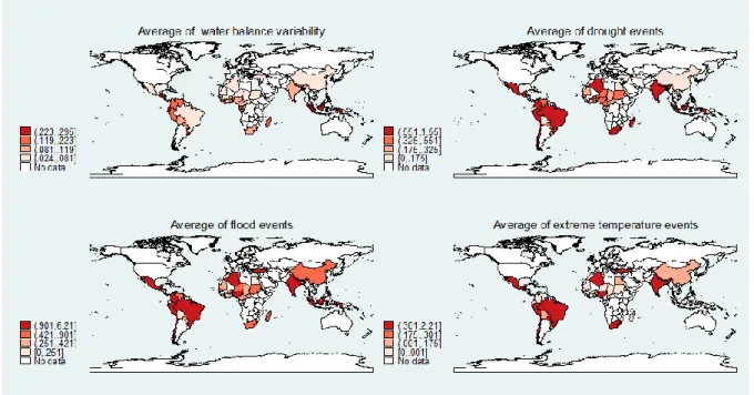
In this paper, climate change is measured by climatic variability and extreme events. Climatic variability is measured by the five-year rolling standard deviation of the growth rate of water balance, which is the difference between precipitation and potential evapotranspiration. Thus, this index combines the impact of climate change on precipitation and temperature and is therefore better suited for analyzing the impact of climate change on agricultural sectors than the simple measure of the variability of rainfall, which is frequently used in the economic literature. The rainfall and evapotranspiration data used to compute water variability come from the Climatic Research Unit (CRU) time-series, Version 3.2 of high resolution gridded data of month-by-month variation in climate.
To analyze extreme climate events affecting food security we use natural disasters data drawn by the Emergency Events Database (EM-DAT) of the Center for Research on the Epidemiology of Disasters (CRED). Natural disasters are defined in the EM-DAT Glossary of Terms as a “situation or event, which overwhelms local capacity,
12
necessitating a request to national or international level for external assistance.” In this study we look at the three natural disasters which are directly related to climate change and most affect food security: drought, flood and extreme temperatures. Each indicator measures the number of events that occurred in a country in a given year as these three natural disasters do not have the same effects on food security. For example, droughts should have a greater negative effect on food security than other natural disasters. Two reasons justify the choice of the number of occurrence of each natural disaster to measure the impact of climate shocks instead of the monetary damage caused by natural disasters or the number of affected people. Indeed, data on monetary damage, number of people affected and the number of deaths are likely to be subject to measurement errors and endogenously determined by the level of development (Skidmore and Toya, 2002). According to Elhorst (2014) it is difficult, if not impossible, to derive Maximum Likelihood (ML) or Bayesian estimators of models with spatial dependence and additional endogenous explanatory variables (Elhorst, 2014). Figure 2 shows the spatial distribution of the climate change indicators of our sample.
The control variables are the main determinants of food security. They include the level of economic development (proxied by the natural logarithm of real GDP per capita), demographic characteristics of the population (logarithm of population
density, logarithm of the dependency ratio1 and logarithm of the population growth
rate), agricultural factors (cereal production land and logarithm of arable land), inflation (consumer prices) and the quality of institutions (polity IV). They are taken from the World Development Indicators (World Bank) and Polity IV project. Descriptive statistics of all of the variables used in the paper are presented in Appendix A.
13
Figure 2: Map of climate change indicators in selected developing countries.
Source: Own calculations using data from CRED (2015).
3.2. Econometric setting
In this study we are primarily interested in the comovement of food availability across countries according to the intensity of their trade relations. This corresponds to a
global2 spatial spillover scenario because a change in supply or demand for food in a
given country will lead to a sequence of adjustments between supply and demand on the international market until a new long term steady state equilibrium is reached. Following Anselin (2001) and Lesage (2014) we therefore estimate a Spatial Durbin
Model (SDM) with fixed effect panel data.3 This model includes spatially lagged
endogenous and exogenous variables and takes into account temporal dimensions and observed and unobserved heterogeneity of countries. In addition, the SDM has the advantage of producing unbiased estimates even if the underlying data generator process is a Spatial Autoregressive Model (Elhorst 2010b). Finally, we separately estimate the impact of climate change indicators as they are strongly correlated. The model to be estimated is written as follows:
2 LeSage (2014) distinguishes between local and global spillovers. Global spillovers arise if spatial
spillovers concern the neighbors of country i, but also the neighbors of its neighbors, and so on. Local spillovers imply only interactions between direct neighbours.
3 Initially, we also try to estimate a Dynamic Spatial Durbin Model with fixed effects but unfortunately
14
𝐹𝑆𝑖𝑡 = 𝜌 𝑊 𝐹𝑆𝐽𝑡+ 𝛼1𝐶𝐶𝑖𝑡+ 𝛼2𝑊𝐶𝐶𝑖𝑡 + 𝛽1𝑋𝑖𝑡+ 𝛽2𝑊𝑋𝑖𝑡+ 𝜇𝑖+ 𝜖𝑖𝑡 (11)
where, 𝐹𝑆𝑖𝑡 is food security, W is the spatial weight matrix, 𝑋𝑖𝑡 the other explanatory
variables (country characteristics : GDP per capita, population density, cereal yields,
arable lands, etc.) in country i at period t and 𝜌 is the spatial autocorrelation
coefficient. 𝐶𝐶𝑖𝑡 is the climatic change variable and our interest variable. 𝛼1, 𝛼2, 𝛽1
and 𝛽2are the parameters to be estimated. 𝜖𝑖𝑡 is the error term in the model and we
allow this error term to be serially correlated. According to the first law of geography: “[E]verything is related to everything else, but near things are more related than distant things” (Tobler, 1970: 236). This law explains why geographical distance has been widely used in spatial econometrics to measure connectivity. However, in a context of market integration, the economic distance matrices are more relevant in certain circumstances. In this study, W is a trade connectivity matrix. It is based on the value of agri-food trade (imports) flows taken from the UN Comtrade database for the period of 1971-2010. Each country is linked to all its trading partners, but the intensity of connectivity is stronger when the share of imports from a country is high. This trade connectivity matrix is more suited to our case study than an inverse distance matrix. Indeed, the availability of food in a country depends more on the volume of imports from other countries than its geographical proximity with these countries. For instance, Burkina Faso is geographically closer to Benin that India, However, a shock on India's rice production (world rice production) will have a greater effect on Burkina Faso than a shock in Benin. We normalize the matrix W by dividing each element (i, j) by the sum of the line.
According to Pace et al. (2012), the use of Instrumental Variables and Generalized Method of Moments to estimate a SDM is less effective than ordinary least squares unless the number of observations is greater than 500,000 because the second order spatially lagged explanatory variables in a SDM are weak instruments and they do not properly identify the spatial autocorrelation coefficient. In this study we use the maximum likelihood method estimator developed by Elhorst (2010a) and Lee and Yu (2010) and implemented in Stata by Hughes and Mortari (2013) to estimate our model.
15
4. Results
4.1. Specification tests
We test the appropriateness of the SDM for analyzing the spatial interdependence of food safety against the Spatial Autoregressive (SAR) model and the Spatial Error Model (SEM). Following Elhorst (2014), we test the joint nullity of all coefficients of
spatially lagged explanatory variables(𝛼2 = 𝛽2 = 0). This test, significant at the 1%
level, allows us to reject the specification SAR. The equality (𝛼2 = −𝜌𝛼1) and
(𝛽2 = −𝜌𝛽1) is rejected by the 𝜒2 at a level of significance of 1% which allows us to
reject the SEM. Finally, the Hausman test is carried out on SDM and allows us to reject the hypothesis of independence between the random effects and explanatory variables. Therefore, the fixed effects model is preferred in this study. All the specification tests are presented at the bottom of Table B.1 in the Appendix.
4.2. General pattern of spatial spillovers
The presence of strategic substitutability in countries' food availability levels in our theoretical model is confirmed by a significant value of the spatial autocorrelation coefficient (𝜌) (table B.1). Put differently, the food availability of a given country tends to decrease along with that of its neighbours. These spillover effects allow for the sharing of world food production between the world's leading food producers and countries with low food production. However, in the case of a global crisis strategic substitutability may also exacerbate food availability and food insecurity by contributing to the leakage to rich countries.
The existence of spatial interactions has important policy implications. Indeed, any change of an explanation variable will generate a direct and an indirect/spillover effects (Lesage and Pace, 2009). The direct effect measures the impact of a change in the value of each explanatory variable in country i on food availability in country j. The indirect effect measures the impact of a change in the value of each explanatory variable in country i on food availability in all other countries (j). Following Lesage (2014), indirect effects capture spillover effects because they arise in all countries but indirect effects decrease with the intensity of trade between countries.
16
4.3. Effect of climate change on food security
The main contribution of this study is the identification of spatial spillover effects of all of the explanatory variables, in general, and more particularly of the impact of climate change. Indeed, we show that the variability of water balance, droughts, floods and extreme temperatures not only negatively affect food availability of the treated/affected country, but also that of its major food trading partners. Table 1 shows that an increase of one point in the variability of the water balance will lead to a of 0.0131g/day/per capita reduction in the country’s food availability and to a 0.0205g /day/per capita reduction in the economic neighborhood for a total effect of 0.0336g/day/per capita. These results are consistent with the predictions of our theoretical model. Previous papers have shown that climatic events have negative effects in the country’s food production (Christensen et al. 2007; Lee et al. 2012), food availability and security (Badolo and Kinda, 2014). However our results are innovative and important because they show that climate events can also reduce food availability in neighbouring countries. Consequently, the omission of the spillover effects in the literature would have led to the underestimation of the climate change effect on food security. In addition, these results allow anticipating the impact of climate indicators that come from partner countries and identifying countries that will be most affected in the future.
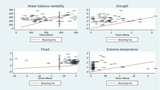
Figure 3 shows the average total impact of climate events (water balance variability, drought, flood, extreme temperatures) by country from 1971 to 2010. It shows that America has suffered more adverse effects of droughts, temperature extremes and variability of water balance while Asia and Africa were more affected by droughts, extreme temperatures and floods. In addition, it also appears that drought events are the most harmful to food availability. Indeed, over the period studied they generated an average decline in food availability of between 0.13 and 0.38g/day/per capita. In addition, figure 4 shows the importance of direct and indirect of climate indicators on per capita food availability in developing countries. The total negative of climate change indicators on food availability in developing countries is more related to indirect effect (spillover effects) than direct effect.
17
Table 1: Climate change and food availability: marginal effects
Food_day_g Food_day_g Food_day_g Food_day_g
Coef. Std. Err. Coef. Std. Err. Coef. Std. Err. Coef. Std. Err.
Direct
Water balance variability -0.0131* (0.0077)
Drought -0.0002*** (0.0001) Flood 0.0000 (0.0001) Extreme temperature -0.0001** (0.0001) Water balance 0.0078** (0.0032) 0.0080*** (0.0029) 0.0082*** (0.0032) 0.0081*** (0.0030) Lgdp 0.0370*** (0.0040) 0.0368*** (0.0038) 0.0367*** (0.0041) 0.0367*** (0.0040) Lpop_dens 0.0755*** (0.0154) 0.0756*** (0.0150) 0.0754*** (0.0162) 0.0754*** (0.0154) Pop_growth -0.0026*** (0.0005) -0.0026*** (0.0005) -0.0026*** (0.0005) -0.0026*** (0.0005) Larable 0.0524*** (0.0042) 0.0524*** (0.0043) 0.0524*** (0.0044) 0.0523*** (0.0043) Cereal_land 0.6711*** (0.0176) 0.6726*** (0.0186) 0.6704*** (0.0177) 0.6715*** (0.0181) Polity2 -0.0104*** (0.0012) -0.0103*** (0.0012) -0.0103*** (0.0012) -0.0103*** (0.0012) LDependency_ratio 0.0738*** (0.0186) 0.0718*** (0.0212) 0.0727*** (0.0220) 0.0719*** (0.0224) Inflation 0.0031*** (0.0008) 0.0028*** (0.0008) 0.0029*** (0.0009) 0.0028*** (0.0008) Indirect
Water balance variability -0.0205* (0.0121)
Drought -0.0004*** (0.0001) Flood -0.0002*** (0.0000) Extreme temperature -0.0002*** (0.0001) Water balance -0.0065 (0.0039) -0.0046 (0.0050) -0.0043 (0.0054) -0.0043 (0.0051) Lgdp -0.0708*** (0.0061) -0.0712*** (0.0067) -0.0713*** (0.0072) -0.0714*** (0.0070) Lpop_dens 0.0110 (0.0304) 0.0096 (0.0306) 0.0100 (0.0321) 0.0098 (0.0307) Pop_growth -0.0080* (0.0046) -0.0071 (0.0048) -0.0075 (0.0053) -0.0072 (0.0051) Larable 0.0150** (0.0072) 0.0158** (0.0078) 0.0157** (0.0080) 0.0156** (0.0077) Cereal_land 0.2595*** (0.0486) 0.2456*** (0.0366) 0.2494*** (0.0337) 0.2455*** (0.0347) Polity2 0.0012 (0.0014) 0.0020 (0.0018) 0.0017 (0.0018) 0.0018 (0.0018) LDependency_ratio -0.0484 (0.0988) -0.0458 (0.0992) -0.0460 (0.1056) -0.0443 (0.1018) Inflation 0.0020 (0.0015) 0.0006 (0.0014) 0.0009 (0.0014) 0.0008 (0.0014) Total
Water balance variability -0.0336*** (0.0116)
Drought -0.0006*** (0.0001) Flood -0.0001*** (0.0000) Extreme temperature -0.0004*** (0.0001) Water balance 0.0014 (0.0012) 0.0033 (0.0023) 0.0039 (0.0025) 0.0038 (0.0023) Lgdp -0.0338*** (0.0024) -0.0345*** (0.0031) -0.0347*** (0.0034) -0.0347*** (0.0031) Lpop_dens 0.0865*** (0.0157) 0.0853*** (0.0163) 0.0853*** (0.0166) 0.0852*** (0.0159) Pop_growth -0.0106** (0.0050) -0.0097* (0.0052) -0.0101* (0.0057) -0.0098* (0.0056) Larable 0.0674*** (0.0036) 0.0682*** (0.0041) 0.0681*** (0.0042) 0.0679*** (0.0039) Cereal_land 0.9306*** (0.0480) 0.9183*** (0.0313) 0.9198*** (0.0288) 0.9170*** (0.0302) Polity2 -0.0092*** (0.0023) -0.0083*** (0.0027) -0.0086*** (0.0028) -0.0085*** (0.0027) LDependency_ratio 0.0253 (0.0827) 0.0260 (0.0806) 0.0267 (0.0860) 0.0276 (0.0816) Inflation 0.0051*** (0.0020) 0.0034** (0.0016) 0.0038** (0.0017) 0.0036** (0.0017)
18
In the literature, climate change can be defined as a change in the trend of the occurrence of climatic phenomena. To measure this change in trend, we compute the difference between the average values of our climate change indicators in the first ten years (1970-1980) of our study and their average values during the last ten years (2001-2010). The results are presented in Table A.3. If the difference is positive then there is an accentuation of the climate phenomenon between the two periods these countries. The higher the value, the higher the impact of climate change on food security has increased between the two periods. These countries are the losers of climate change. In contrast, if the difference is negative then there has been a reduction in the occurrence of climatic phenomenon between the two sub-periods. The countries that are in this situation have benefited from a reduction of the negative effects of climate change between the two periods.
For each country, we can compute the direct and indirect effects of the change in the trend of indicators of climate change on food security by multiplying the marginal effects (direct and indirect) by this trend. The impact of the change in trend of climate change indicators on food availability by country is presented in Figure 5. This graph shows different pictures. In South America and Africa, the impact of water balance variability on food availability has increased between the two sub-periods. In addition Africa, India, Nepal, and Southeast Asia are those that experienced the largest increases in the impact of droughts. In contrast the impact of flooding has increased especially in Asia and Africa. Finally, India, China, South Africa, Central America, Brazil and Bolivia are those who have known a sharp rise of the impact of extreme temperatures on food availability. Final, figure 6 concludes that the marginal contribution of spillover effects of the trend of climate change indicators is higher than the direct effect.
19
Figure 3: Map of the average decline in per capita food availability caused by climate change indicators (1971-2010).
Source: Own calculations.
Figure 4: Average marginal impact (direct and indirect) of climate change indicators on per capita food availability.
Source: Own calculations.
BDI BEN BFA BOL BRA CAF CHL CHN CIV CMR COG COL CRI DOM DZA ECU EGY GAB GHA GTM HND HUN IDN IND KOR LBR LKA MAR MDG MEX MRT MYS NER NGA NIC NPL PAN PER PHL PRY RWA SDN SEN SLE SYR TCD TGO TTO TUN TUR URY VEN ZAF 0 .001 .002 .003 .004 .005 In d ir e c t e ff e c ts 0 .001 .002 .003 .004 Direct effects Bisecting line
Water balance variability
BDI BEN BFA BOL BRA CAF CHL CHN CIV CMR COG COL CRI DOM DZA ECU EGY GAB GHA GTM HND HUN IDN IND KOR LBR LKA MAR MDG MEX MRT MYS NER NGA NIC NPL PAN PER PHL PRY RWA SDN SEN SLE SYRTGO TCD TTO TUN TUR URY VEN ZAF 0 .1 .2 .3 .4 .5 In d ir e c t e ff e c ts 0 .1 .2 .3 Direct effects Bisecting line Drought BDI BEN BFA BOL BRA CHL CAF CHN CIV CMRCOG COL DOM CRI
DZA ECU EGY GAB GHA GTM HND HUN IDN IND KOR LBR LKA MAR MDG MEX MRT MYS NER NGA NIC NPL PAN PER PHL PRY RWA SDNSEN SLESYR TCDTGO TTO TUN TUR URY VEN ZAF -.5 0 .5 1 In d ir e c t e ff e c ts -.25 -.2 -.15 -.1 -.05 0 Direct effects Bisecting line Flood BDI BEN BFA BOL BRA CAF CHL CHN CIV CMR COG COL CRI DOM DZA ECU EGY GAB GHA GTM HND HUN IDN IND KOR LBR LKA MAR MDG MEX MRT MYS NER NGA NIC PAN PHL PRY RWA SDN SEN SLE SYR TCD TGO TTO TUN TUR URY VEN 0 .1 .2 .3 .4 In d ir e c t e ff e c ts 0 .05 .1 .15 .2 Direct effects Bisecting line Extreme temperature
20
Figure 5: Map of the impact of climate change (change in trend) on food availability per capita.
Source: Own calculations.
Figure 6: Average marginal impact (direct and indirect) of the trend of climate change indicators on per capita food availability.
Source: Own calculations.
BDI BEN BFA BOL BRA CAF CHL CHN CIV COGCMR COL CRI DOM DZA ECU EGY GAB GHA GTM HND IDNHUN IND KOR LBR LKA MAR MDG MEXMRT MYS NER NGA NIC NPL PAN PER PHL PRY RWA SDN SEN SLE SYR TCD TGO TTO TUN TUR URY VEN ZAF -.001 0 .001 .002 .003 In d ir e c t e ff e c ts -.001 0 .001 .002 .003 Direct effects Bisecting line
Trend of water balance variability
BDI BENBFA BOL BRA CAF CHLCHNCIV CMRCOG COL CRI DOM DZA ECU EGY GABGHA GTM HND HUN IDN IND KOR LBR LKA MAR MDG MEX MRT MYS NER NGA NIC NPL PAN PER PHL PRY RWA SDN SEN SLE SYR TCD TGO TTO TUNTUR URY VEN ZAF -.4 -.2 0 .2 .4 .6 In d ir e c t e ff e c ts -.4 -.2 0 .2 .4 .6 Direct effects Bisecting line Trend of drought BDI BEN BFA BOL BRA CAF CHL CHN CIV CMR COG COL CRI DOM DZA ECU EGY GAB GHA GTM HND HUN KOR LBR LKA MAR MDG MEX MRT NER NGA NIC NPL PAN PER PHL PRY RWA SDN SEN SLE SYR TCDTGO TTO TUN TUR URY VEN ZAF -.2 0 .2 .4 .6 In d ir e c t e ff e c ts -.2 -.1 0 .1 Direct effects Bisecting line Trend of flood BDI BEN BFA BOL BRA CAF CHL CHN CIV CMR COG COL CRI DOM DZA ECU EGY GAB GHA GTM HND HUN IDN IND KOR LBR LKA MAR MDG MEX MRT MYS NER NGA NIC PAN PHL PRY RWA SDN SEN SLE SYR TCD TGO TTO TUN TUR URY VEN 0 .05 .1 .15 In d ir e c t e ff e c ts 0 .05 .1 .15 Direct effects Bisecting line
21
4.4. Spillover effects and explanatory variables
The percentage of arable land and the area of land devoted to cereal production in a given country increase the food availability both of this country and of its major trading partners. The water balance and percentage of people of working age (dependency ratio) have a direct positive effect on food availability and a non-significant indirect effect. These results validate proposition 2 of the theoretical model. GDP per capita has a positive direct effect and negative indirect effect on food availability. In other words, economic resources improve the capacity of a given country to increase food availability. However an increase of GDP per capita from its major trading partner countries can reduce this food availability through food imports. This expected effect is consistent with the predictions of proposition 3. Contrariwise, density of population and inflation have a significant positive direct effect and a non-significant indirect effect. The sign of the direct effect is in line with our expectations. Indeed, an increase in demand (population density) or prices (inflation) will boost food supply and lead to an increase in food availability through imports. The population growth rate has both a direct and an indirect negative and significant effect on food availability. This result seems intuitive because population growth increases pressure on world agricultural resources. Finally, democracy has a counter-intuitive direct effect. It has a negative direct impact on food security in the country while the indirect effect has the expected positive impact.
4.5. Robustness checks
In this section, we test whether our results are robust to the inclusion of all food commodities in the calculation of food availability and to a change of the econometric specification used.
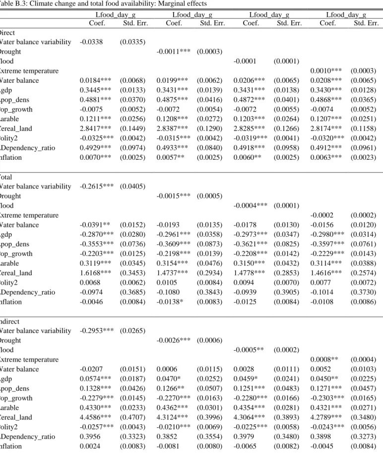
First, in the case of climatic events affecting cereal production, countries may substitute cereals with other foods. In this case, the reduction of cereal availability will have no effect on total food availability. As a robustness check, we repeat the analysis using the total food availability (expressed in kilocalories/person/year) as the dependent variable instead of cereal availability. The results, reported in Table B.2 and B.3 in the Appendix, confirm strategic substitutability between food availability
22
levels and the negative effect of climate change on food security. Indeed, the direct and indirect effects associated with climate change variables are negative and significantly different from zero, except for the direct effect of the variability of the water balance. Furthermore, the spatial autocorrelation coefficient is negative and significantly different from zero at the 1% level, although it is relatively lower.
Second, methodologically, our use of the SDM is the most suitable model to analyze the spatial interdependence of the level of food availability between countries; however, the error terms of this model can be spatially correlated. This correlation can be explained by the omission of spatially correlated explanatory variables such as climatic, hydrological and soil fertility factors. In addition, neighboring countries are more likely to use similar agricultural practices, which could also lead to a spatial correlation of the error term. This spatial correlation is more related to geographical proximity than to commercial relations between countries. According to Lesage (2014), who equates these spatial interactions to local spillovers, a neighborhood matrix is more suitable for this analysis. Thus, we consider a general nesting spatial model with a spatially lagged dependent variable (economic matrix W), spatially lagged explanatory variables and spatially correlated error term (geographical
neighborhood matrix𝑊2). The use of a different neighborhood matrix between the
dependent variable and the error term facilitated the identification of this model (Elhorst, 2014). The estimated model is written as follows:
𝐹𝑆𝑖𝑡 = 𝜌 𝑊 𝐹𝑆𝐽𝑡+ 𝛼1𝐶𝐶𝑖𝑡+ 𝛼2𝑊𝐶𝐶𝑖𝑡 + 𝛽1𝑋𝑖𝑡+ 𝛽2𝑊𝑋𝑖𝑡+ 𝜇𝑖 + 𝜆𝑊2𝑢𝑗𝑡+ 𝜖𝑖𝑡 (12)
With 𝑊2 the matrix of 5 nearest neighbors, 𝜆 the spatial autocorrelation coefficient of
error terms and 𝑊2𝑢𝑗𝑡 is referred to as the spatially-lagged error.
The results presented in Table B.4 in the Appendix show that the spatial autocorrelation coefficient of the error terms is not significant. This reinforces both our choice of the SDM in this study and the nature of spatial interactions that we have highlighted.
23
5. Concluding remarks
Global warming poses considerable uncertainty on agricultural production and food availability and, thus, on the livelihoods of the most vulnerable populations. Therefore rigorous analyses based on improved methodologies are needed to inform public decisions.
In this article we theoretically and empirically investigate the existence of spatial interactions between the levels of food availability of countries and analyse the spatial spillover effects of climatic change (water balance variability, droughts, floods and extreme temperatures) on food availability. Our contribution to theory is the modeling of the impact of shocks and the spillover effects that result using a Samuelson’s spatial price equilibrium model. We empirically use a Spatial Durbin Model in which the spatial interdependence of food availability levels between the countries is explicitly modeled using a trade connectivity matrix (imports of food commodities). Results are as follows: firstly we show that the level of food availability in a given country is a strategic substitute of those of its main trading partners. In other words, an increase of food availability in a given country reduces the food availability of its main trading partners. Second, climatic events (water balance variability, droughts, floods and extreme temperatures) have spillover effects. Indeed they reduce food availability in both the country and in its economic neighborhood. The adverse effect of climate change on food availability in developing countries is more explained by spillover effects than direct effects. Third, results establish that demand factors (income per capita, population density, population growth, dependence ratio) in a country may have the opposite (asymmetric) effect on its major trading partners. Final, the effect of supply factors (water balance variability, drought, flood, extreme temperature, water balance, arable and cereal lands,) on food availability is symmetric.
Our results have clear policy implications. A better knowledge about the nature of the spatial effects of climate change can improve the design and implementation of climate policies aimed at fighting against food insecurity in developing countries. Indeed, instead of the emergency response strategy against food insecurity, our results suggest to establish mechanisms that identify countries that most are affected and vulnerable to climate change. In addition, mitigation and adaptation policies could be
24
implemented to countries by taking into account the spatial spillover effects of climate change. In other words, because the vulnerability depends on the type of climate events that developing countries are exposed to, they could identify and implement policies that serve multiple objectives (development, adaptation and mitigation). These strategies may contribute to circumscribe the impact of climate change on food security, but also to anticipate, plan and optimize food safety policies.
25
References
Adams, R. 1989. Global climate change and agriculture: an economic perspective.
American Journal of Agricultural Economics, 71(5): 1272–1279.
Barrett, C.B. and Li, J.R. 2002. Distinguishing Between Equilibrium and Integration in Spatial Price Analysis. American Journal of Agricultural Economics, 84, 292-307. Baulch, R.J. 1997. Transfer Costs, Spatial Arbitrage, and Testing for Food Market Integration. American Journal of Agricultural Economics, 79, 477-487.
Badolo, F., and Kinda S. R. 2014. Climatic Variability and Food Security in
Developing Countries. Working Paper halshs-00939247. HAL.
http://ideas.repec.org/p/hal/wpaper/halshs-00939247.html.
Christensen et al. 2007. Climate change 2007: The physical science basis. Agenda 6: 07.
Deschênes, O. and Greenstone, M. 2007. The economic impacts of climate change: evidence from agricultural output and random fluctuations in weather. American
Economic Review, 97(1): 354–385.
Eckersten, H., K. Blombäck, T. Kätterer & P. Nyman. 2001. Modelling C, N, water and heat dynamics in winter wheat under climate change in southern Sweden.
Agriculture Ecosystems & Environment, 142: 6-17.
Elhorst P., 2010a. Spatial Panel Data Models. Handbook of applied spatial analysis. Edited by Fisher, M.M., Getis, A.
Elhorst, P., 2010b. Applied spatial econometrics: Raising the bar. Spatial Economic Analysis, 5:1, 9-28.
FAO. 2008. Crop Prospects and Food Situation - No. 2, April 2008. http://www.fao.org/docrep/010/ai465e/ai465e00.htm
FAO. 2009. The State of Food Insecurity in the World. Economic crises - impacts and lessons learned. The FAO Report. Rome.
Goodwin, B.K et Pigott, N.E. 2001. Spatial market integration in the Presence of threshold Effects. American Journal of Agricultural Economics, 83, 302-317
Hughes G. and Mortari A. P., 2013. A Command to Estimate Spatial Panel Models in Stata. German Stata Users’ Group Meetings 2013.
IPCC, Climate change 2007. Synthesis report. https://www.ipcc.ch/pdf/assessment-report/ar4/syr/ar4_syr.pdf
Lee, Jaehyuk, Denis A. Nadolnyak, et Valentina M. Hartarska. 2012. Impact of Climate Change on Agricultural Production in Asian Countries: Evidence from Panel
26
Study. 2012 Annual Meeting, February 4-7, 2012, Birmingham, Alabama 119808.
Southern Agricultural Economics Association.
http://ideas.repec.org/p/ags/saea12/119808.html.
Lee L.-F., Yu J., 2010. Estimation of spatial autoregressive panel data models with fixed effects. Journal of Econometrics, 154, 165-185.
LeSage, J.P., 2014. What regional scientists need to know about spatial econometrics,
Rochester, NY: Social Science Research Network. Available at: http ://papers.ssrn.com/sol3/Papers.cfm?abstractid = 2420725
Pace K., LeSage J. and Zhu S., 2012. Spatial Dependence in Regressors. Advances in
Econometrics Volume 30, Thomas B. Fomby, R. Carter Hill, Ivan Jeliazkov, Juan
Carlos Escanciano and Eric Hillebrand (Series Eds., Volume editors: Dek Terrell and Daniel Millimet) , 2012, 257-295.)
Ravallion, M. 1986. Testing Market Integration. American Journal of Agricultural
Economics, 68, 102-109.
Ringler, C., Zhu, T., Cai, X., Koo, J. and Wang D. 2010. Climate Change Impacts on
Food Security in Sub-Saharan Africa. IFPRI Discussion Paper 01042.
Schlenker, W., Hanemann, W. and Fisher, A. 2005. Will US agriculture really benefit from global warming? Accounting for irrigation in the hedonic approach. American
Economic Review, 95(1): 395–406.
Skidmore, M. Toya, H. 2007. Economic development and the impacts of natural disasters. Economic Letters, 94, 20-25.
St.Clair, S., B., Lynch J. P. 2010. The opening of Pandora’s Box: climate change impacts on soil fertility and crop nutrition in developing countries. Plant and Soil, 335 (1-2): 101‑15. doi:10.1007/s11104-010-0328-z.
Von-Braun, J. 1991. A policy agenda for famine prevention in Africa. Food policy
reports 1. International Food Policy Research Institute (IFPRI).
27
Appendix
A. Description, data sources and list of countries
Table A.1. Description and data sources
Variable Description Source Mean Std. Dev.
Food_day_g Refers to the total amount of the
commodity available as human food during the reference period. Food availability is the total of food production + food import- food exports+ variation in food stocks.
FAO(2015)
0.360 0.137
Water balance variability Measured by the five-year rolling
standard deviation of the growth rate of the water balance, this is the difference between precipitation and potential evapotranspiration (in thousand square millimeters).
Climatic Research Unit (2015)
0.141 0.102
Drought Number of occurrence of drought
events per year.
CRED (2015)
0.391 2.304
Flood Number of occurrence of flood
events per year.
CRED (2015)
0.779 5.436
Extreme temperature Number of occurrence of extreme
temperature events by year
CRED (2015)
0.230 2.422
Water balance Yearly average water balance (in
thousand millimeters).
Climatic Research
Unit (2015) -0.050 1.053
Lgdp Logarithm of GDP per capita
(constant 2005 US$)
WDI (2015)
7.139 1.120
Lpop_dens Logarithm of population density WDI (2015) 3.643 1.242
Pop_growth Population growth rate WDI (2015) 2.221 1.004
Larable Percentage of arable lands WDI (2015) 2.132 1.039
Cereal_land Land under cereal production in
millions of hectares.
WDI (2015)
0.062 0.183
Polity2 The Polity Score captures the
regime authority spectrum on a 21-point scale ranging from -10 (hereditary monarchy) to +10 (consolidated democracy).
Polity IV (2010)
0.018 1.000
LDependency_ratio Logarithm of the proportion of
people between the ages of 15 and 65
WDI (2015)
4.022 0.093
28 Table A.2. List of countries
Algeria Gabon Panama
Benin Ghana Paraguay
Bolivia Guatemala Peru
Brazil Honduras Philippines
Burkina Faso Hungary Rwanda
Burundi India Senegal
Cameroon Indonesia Sierra Leone
Central African
Republic Korea, Rep. South Africa
Chad Liberia Sri Lanka
Chile Madagascar Sudan
China Malaysia Syrian Arab Republic
Colombia Mauritania Togo
Congo, Rep. Mexico Trinidad and Tobago
Costa Rica Morocco Tunisia
Cote d'Ivoire Nepal Turkey
Dominican Republic Nicaragua Uruguay
Ecuador Niger Venezuela
29
Table A.3. : Average (1971-1980 and 2001-2010) and trend of climate change indicators by country
Water Balance
variability Drought occurrence Flood occurrence
Extreme temperature occurrence
Country 71-80 01-10 Change 71-80 01-10 Change 71-80 01-10 Change 71-80 01-10 Change
Algeria 0.020 0.028 0.008 0.000 0.000 0.000 0.000 0.000 0.000 0.000 0.000 0.000 Benin 0.093 0.111 0.018 0.100 0.600 0.500 0.100 0.600 0.500 0.000 0.000 0.000 Bolivia 0.073 0.095 0.022 0.000 0.200 0.200 0.000 0.300 0.300 0.000 0.200 0.200 Brazil 0.061 0.072 0.011 0.200 0.300 0.100 0.500 0.400 -0.100 0.300 0.600 0.300 Burkina Faso 0.056 0.106 0.050 0.100 0.800 0.700 0.100 0.900 0.800 0.000 0.000 0.000 Burundi 0.095 0.145 0.050 0.100 0.300 0.200 0.100 0.400 0.300 0.000 0.000 0.000 Cameroon 0.075 0.087 0.012 0.000 0.600 0.600 0.000 0.600 0.600 0.000 0.000 0.000
Central African Rep. 0.090 0.057 -0.033 0.000 1.000 1.000 0.000 1.100 1.100 0.000 0.000 0.000
Chad 0.034 0.036 0.002 0.100 0.800 0.700 0.200 1.000 0.800 0.000 0.000 0.000 Chile 0.059 0.096 0.038 0.000 0.000 0.000 0.000 0.000 0.000 0.000 0.000 0.000 China 0.031 0.039 0.008 0.000 0.200 0.200 0.000 1.700 1.700 0.000 0.200 0.200 Colombia 0.140 0.236 0.097 0.000 0.000 0.000 0.000 0.000 0.000 0.000 0.000 0.000 Congo, Rep. 0.110 0.098 -0.012 0.000 0.700 0.700 0.000 0.800 0.800 0.000 0.000 0.000 Costa Rica 0.255 0.269 0.014 0.000 0.000 0.000 0.000 0.000 0.000 0.000 0.000 0.000 Cote d'Ivoire 0.139 0.094 -0.045 0.100 0.600 0.500 0.100 0.600 0.500 0.000 0.000 0.000 Dominican Republic 0.204 0.242 0.037 0.100 0.100 0.000 0.100 0.100 0.000 0.000 0.000 0.000 Ecuador 0.197 0.275 0.079 0.100 0.200 0.100 0.100 0.200 0.100 0.000 0.000 0.000
Egypt, Arab Rep. 0.022 0.022 0.001 0.000 0.000 0.000 0.000 0.300 0.300 0.000 0.200 0.200
Gabon 0.119 0.101 -0.018 0.000 0.000 0.000 0.000 0.300 0.300 0.000 0.000 0.000 Ghana 0.171 0.115 -0.056 0.100 0.200 0.100 0.100 0.300 0.200 0.000 0.000 0.000 Guatemala 0.269 0.246 -0.023 0.000 0.100 0.100 0.000 0.100 0.100 0.000 0.100 0.100 Honduras 0.275 0.190 -0.085 0.000 1.600 1.600 0.000 2.200 2.200 0.000 0.000 0.000 Hungary 0.120 0.139 0.020 0.000 0.100 0.100 0.000 0.200 0.200 0.000 0.100 0.100 India 0.115 0.068 -0.047 0.300 0.600 0.300 0.800 2.300 1.500 0.300 0.600 0.300 Indonesia 0.296 0.297 0.001 0.200 3.500 3.300 1.000 15.30 14.30 0.000 0.000 0.000 Korea, Rep. 0.225 0.335 0.110 0.000 0.200 0.200 0.000 0.200 0.200 0.000 0.200 0.200 Liberia 0.260 0.190 -0.070 0.000 0.400 0.400 0.000 0.400 0.400 0.000 0.400 0.400 Madagascar 0.130 0.093 -0.037 0.000 0.300 0.300 0.000 0.400 0.400 0.000 0.000 0.000 Malaysia 0.212 0.373 0.161 0.100 0.300 0.200 0.100 0.500 0.400 0.000 0.000 0.000 Mauritania 0.027 0.030 0.003 0.000 0.100 0.100 0.000 0.100 0.100 0.000 0.000 0.000 Mexico 0.046 0.049 0.003 0.000 0.100 0.100 0.000 0.100 0.100 0.000 0.100 0.100 Morocco 0.077 0.107 0.030 0.000 0.000 0.000 0.000 0.000 0.000 0.000 0.000 0.000 Nepal 0.148 0.127 -0.021 0.000 1.900 1.900 0.000 2.600 2.600 0.000 2.000 2.000 Nicaragua 0.248 0.322 0.074 0.000 0.100 0.100 0.000 0.100 0.100 0.000 0.000 0.000 Niger 0.038 0.051 0.012 0.100 0.900 0.800 0.100 1.200 1.100 0.000 0.000 0.000 Nigeria 0.074 0.069 -0.005 0.000 0.800 0.800 0.000 2.000 2.000 0.000 0.800 0.800 Panama 0.164 0.255 0.091 0.000 1.900 1.900 0.000 2.800 2.800 0.000 0.000 0.000 Paraguay 0.135 0.168 0.033 0.000 1.400 1.400 0.000 1.500 1.500 0.000 1.400 1.400 Peru 0.091 0.126 0.035 2.400 0.100 -2.300 3.400 0.300 -3.100 2.400 0.100 -2.300 Philippines 0.285 0.385 0.099 0.200 0.300 0.100 0.200 2.600 2.400 0.000 0.000 0.000 Rwanda 0.091 0.136 0.045 0.100 0.400 0.300 0.100 0.500 0.400 0.000 0.000 0.000 Senegal 0.112 0.122 0.010 0.100 0.400 0.300 0.100 0.400 0.300 0.000 0.000 0.000 Sierra Leone 0.170 0.106 -0.064 0.000 0.000 0.000 0.000 0.500 0.500 0.000 0.000 0.000 South Africa 0.081 0.109 0.028 0.000 2.600 2.600 0.000 3.300 3.300 0.000 2.600 2.600 Sri Lanka 0.262 0.186 -0.076 0.100 0.300 0.200 0.100 0.400 0.300 0.000 0.000 0.000 Sudan 0.032 0.048 0.017 0.100 0.900 0.800 0.100 1.100 1.000 0.000 0.000 0.000
Syrian Arab Republic 0.103 0.086 -0.017 0.300 0.000 -0.300 0.300 0.000 -0.300 0.000 0.000 0.000
Togo 0.114 0.144 0.030 0.000 0.400 0.400 0.000 0.400 0.400 0.000 0.000 0.000
Trinidad and Tobago 0.143 0.219 0.075 0.000 0.000 0.000 0.000 0.000 0.000 0.000 0.000 0.000
Tunisia 0.074 0.070 -0.003 0.100 0.000 -0.100 0.200 0.000 -0.200 0.000 0.000 0.000
Turkey 0.076 0.065 -0.011 0.000 0.000 0.000 0.400 0.300 -0.100 0.200 0.100 -0.100
Uruguay 0.172 0.255 0.083 0.000 0.000 0.000 0.000 0.000 0.000 0.000 0.000 0.000
30
B. Empirical Results
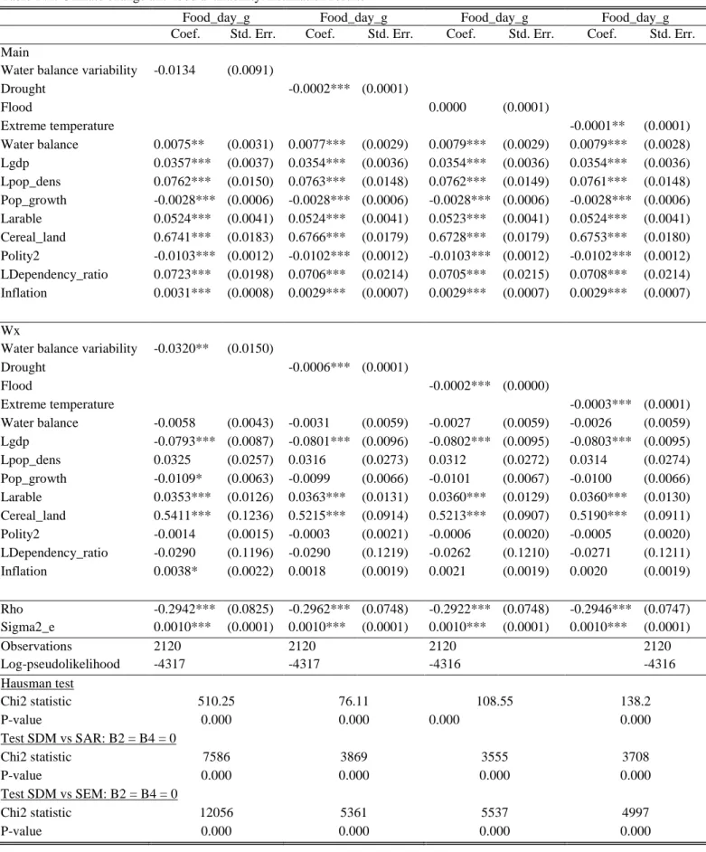
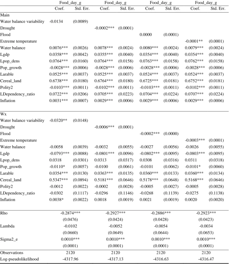
Table B.1: Climate change and food availability: Estimation results
Food_day_g Food_day_g Food_day_g Food_day_g
Coef. Std. Err. Coef. Std. Err. Coef. Std. Err. Coef. Std. Err.
Main
Water balance variability -0.0134 (0.0091)
Drought -0.0002*** (0.0001) Flood 0.0000 (0.0001) Extreme temperature -0.0001** (0.0001) Water balance 0.0075** (0.0031) 0.0077*** (0.0029) 0.0079*** (0.0029) 0.0079*** (0.0028) Lgdp 0.0357*** (0.0037) 0.0354*** (0.0036) 0.0354*** (0.0036) 0.0354*** (0.0036) Lpop_dens 0.0762*** (0.0150) 0.0763*** (0.0148) 0.0762*** (0.0149) 0.0761*** (0.0148) Pop_growth -0.0028*** (0.0006) -0.0028*** (0.0006) -0.0028*** (0.0006) -0.0028*** (0.0006) Larable 0.0524*** (0.0041) 0.0524*** (0.0041) 0.0523*** (0.0041) 0.0524*** (0.0041) Cereal_land 0.6741*** (0.0183) 0.6766*** (0.0179) 0.6728*** (0.0179) 0.6753*** (0.0180) Polity2 -0.0103*** (0.0012) -0.0102*** (0.0012) -0.0103*** (0.0012) -0.0102*** (0.0012) LDependency_ratio 0.0723*** (0.0198) 0.0706*** (0.0214) 0.0705*** (0.0215) 0.0708*** (0.0214) Inflation 0.0031*** (0.0008) 0.0029*** (0.0007) 0.0029*** (0.0007) 0.0029*** (0.0007) Wx
Water balance variability -0.0320** (0.0150)
Drought -0.0006*** (0.0001) Flood -0.0002*** (0.0000) Extreme temperature -0.0003*** (0.0001) Water balance -0.0058 (0.0043) -0.0031 (0.0059) -0.0027 (0.0059) -0.0026 (0.0059) Lgdp -0.0793*** (0.0087) -0.0801*** (0.0096) -0.0802*** (0.0095) -0.0803*** (0.0095) Lpop_dens 0.0325 (0.0257) 0.0316 (0.0273) 0.0312 (0.0272) 0.0314 (0.0274) Pop_growth -0.0109* (0.0063) -0.0099 (0.0066) -0.0101 (0.0067) -0.0100 (0.0066) Larable 0.0353*** (0.0126) 0.0363*** (0.0131) 0.0360*** (0.0129) 0.0360*** (0.0130) Cereal_land 0.5411*** (0.1236) 0.5215*** (0.0914) 0.5213*** (0.0907) 0.5190*** (0.0911) Polity2 -0.0014 (0.0015) -0.0003 (0.0021) -0.0006 (0.0020) -0.0005 (0.0020) LDependency_ratio -0.0290 (0.1196) -0.0290 (0.1219) -0.0262 (0.1210) -0.0271 (0.1211) Inflation 0.0038* (0.0022) 0.0018 (0.0019) 0.0021 (0.0019) 0.0020 (0.0019) Rho -0.2942*** (0.0825) -0.2962*** (0.0748) -0.2922*** (0.0748) -0.2946*** (0.0747) Sigma2_e 0.0010*** (0.0001) 0.0010*** (0.0001) 0.0010*** (0.0001) 0.0010*** (0.0001) Observations 2120 2120 2120 2120 Log-pseudolikelihood -4317 -4317 -4316 -4316 Hausman test Chi2 statistic 510.25 76.11 108.55 138.2 P-value 0.000 0.000 0.000 0.000 Test SDM vs SAR: B2 = B4 = 0 Chi2 statistic 7586 3869 3555 3708 P-value 0.000 0.000 0.000 0.000 Test SDM vs SEM: B2 = B4 = 0 Chi2 statistic 12056 5361 5537 4997 P-value 0.000 0.000 0.000 0.000
31 Standard errors in parentheses; * p<0.10, * p<0.05, * p<0.01.
Table B.2: Climate change and total food availability: Estimation results
Lfood_day_g Lfood_day_g Lfood_day_g Lfood_day_g
Coef. Std. Err. Coef. Std. Err. Coef. Std. Err. Coef. Std. Err.
Main
Water balance variability -0.0345 (0.0395)
Drought -0.0011*** (0.0003) Flood -0.0001 (0.0001) Extreme temperature 0.0010*** (0.0003) Water balance 0.0178*** (0.0063) 0.0194*** (0.0059) 0.0201*** (0.0059) 0.0203*** (0.0058) Lgdp 0.3420*** (0.0133) 0.3408*** (0.0127) 0.3408*** (0.0127) 0.3409*** (0.0126) Lpop_dens 0.4855*** (0.0417) 0.4842*** (0.0413) 0.4842*** (0.0415) 0.4848*** (0.0412) Pop_growth -0.0093* (0.0056) -0.0091 (0.0056) -0.0091 (0.0056) -0.0092 (0.0056) Larable 0.1221*** (0.0282) 0.1221*** (0.0276) 0.1217*** (0.0276) 0.1212*** (0.0275) Cereal_land 2.8415*** (0.1587) 2.8390*** (0.1335) 2.8275*** (0.1306) 2.8172*** (0.1278) Polity2 -0.0320*** (0.0042) -0.0311*** (0.0044) -0.0314*** (0.0043) -0.0316*** (0.0043) LDependency_ratio 0.5010*** (0.0971) 0.4936*** (0.0964) 0.4941*** (0.0963) 0.4941*** (0.0968) Inflation 0.0065*** (0.0025) 0.0053** (0.0024) 0.0056** (0.0025) 0.0060** (0.0024) Wx
Water balance variability -0.2802*** (0.0428)
Drought -0.0017*** (0.0004) Flood -0.0004*** (0.0001) Extreme temperature -0.0001 (0.0003) Water balance -0.0394** (0.0167) -0.0177 (0.0130) -0.0161 (0.0128) -0.0140 (0.0126) Lgdp -0.2793*** (0.0318) -0.2887*** (0.0365) -0.2896*** (0.0363) -0.2913*** (0.0360) Lpop_dens -0.3387*** (0.0842) -0.3465*** (0.0898) -0.3475*** (0.0896) -0.3475*** (0.0890) Pop_growth -0.2406*** (0.0178) -0.2377*** (0.0190) -0.2384*** (0.0190) -0.2406*** (0.0190) Larable 0.3453*** (0.0465) 0.3422*** (0.0509) 0.3408*** (0.0497) 0.3374*** (0.0497) Cereal_land 1.9777*** (0.5006) 1.7693*** (0.3485) 1.7664*** (0.3428) 1.7512*** (0.3378) Polity2 0.0035 (0.0062) 0.0079 (0.0081) 0.0067 (0.0078) 0.0050 (0.0083) LDependency_ratio -0.0893 (0.4326) -0.1100 (0.4348) -0.1040 (0.4305) -0.1052 (0.4294) Inflation -0.0036 (0.0082) -0.0138 (0.0086) -0.0124 (0.0082) -0.0104 (0.0084) Rho -0.0867*** (0.0334) -0.0739** (0.0294) -0.0720** (0.0295) -0.0705** (0.0295) Sigma2_e 0.0201*** (0.0026) 0.0201*** (0.0026) 0.0202*** (0.0026) 0.0201*** (0.0026) Observations 2040 2040 2040 2040 Log-pseudolikelihood -1087 -1087 -1088 -1091