HAL Id: hal-02933792
https://hal.archives-ouvertes.fr/hal-02933792v2
Preprint submitted on 7 May 2021
HAL is a multi-disciplinary open access
archive for the deposit and dissemination of
sci-entific research documents, whether they are
pub-lished or not. The documents may come from
teaching and research institutions in France or
abroad, or from public or private research centers.
L’archive ouverte pluridisciplinaire HAL, est
destinée au dépôt et à la diffusion de documents
scientifiques de niveau recherche, publiés ou non,
émanant des établissements d’enseignement et de
recherche français ou étrangers, des laboratoires
publics ou privés.
A stable Spectral Difference approach for computations
with triangular and hybrid grids up to the 6th order of
accuracy
Adèle Veilleux, Guillaume Puigt, Hugues Deniau, Guillaume Daviller
To cite this version:
Adèle Veilleux, Guillaume Puigt, Hugues Deniau, Guillaume Daviller. A stable Spectral Difference
approach for computations with triangular and hybrid grids up to the 6th order of accuracy. 2021.
�hal-02933792v2�
A stable Spectral Difference approach for computations with
triangular and hybrid grids up to the 6
th
order of accuracy
Ad`ele Veilleux
∗,1,2, Guillaume Puigt
†,1, Hugues Deniau
‡,1, Guillaume Daviller
§,21 ONERA/DMPE, Universit´e de Toulouse, F-31055 Toulouse, France
2 Centre Europ´een de Recherche et de Formation Avanc´ee en Calcul Scientifique (CERFACS),
42 avenue Gaspard Coriolis, 31057 Toulouse Cedex 01, France Abstract
In the present paper, a stable Spectral Difference formulation on triangles is defined using a flux polynomial expressed in the Raviart-Thomas basis up to the sixth-order of accuracy. Compared to the literature on the Spectral Difference approach, the present work increases the order of accuracy that the stable formulation can deal with. The proposed scheme is based on a set of flux points defined in the paper. The sets of points leading to a stable formulation are determined using a Fourier stability analysis of the linear advection equation coupled with an optimization process. The proposed Spectral Difference formulation differs from the Flux Reconstruction method on hybrid grids: the distinction between the two approaches is highlighted through the definition of the number of interior flux points. Validation starts from a convergence study using Euler equations and continues with the simulation of laminar viscous flows over the NACA0012 airfoil using quadratic triangles and of the laminar flow around a cylinder using a hybrid grid.
Keyword: high-order method, Spectral Difference method, Raviart-Thomas space, triangle, hybrid, linear stability analysis.
1
Introduction
Many advancements in high-order discontinuous methods enable accurate and robust simulations on un-structured grids with a good parallel efficiency. Numerical schemes using piecewise continuous polynomials are widely used to obtain high-order accuracy. The aim is to look for a polynomial solution in each mesh cell, but without requiring the solution to be continuous across mesh interfaces. The most popular approach, the Discontinuous Galerkin (DG) method, was successfully implemented in many solvers and leads to very rich research. Without being exhaustive, a partial literature review focused on Computational Fluid Dy-namics is available in several books [1, 2, 3, 4, 5, 6, 7, 8] and many contributions in Europe also come from projects [9, 10, 11] involving research centers and industry [12]. The DG method links the standard Finite Element method and the Finite Volume method: unknowns defined on a polynomial basis are solution of a weak problem as in Finite Element but discontinuities at mesh interfaces are solved using an approximated Riemann solver as in Finite Volume. While DG methods are based on the integral form of equations, other methods directly use the strong form, which results in a simpler formulation and implementation as well as a lower computational cost since no integral needs to be computed [13]. For a standard hyperbolic equation, the solution is sought under the form of a polynomial of degree p defined in any mesh cell. For consistency, it is mandatory to define the flux density divergence as a polynomial of degree p since dealing with the strong formulation means that the divergence of the flux polynomial is explicitly computed. Today, there are essentially two classes of methods based on the strong formulation.
∗Corresponding author, Adele.Veilleux@onera.fr †Guillaume.Puigt@onera.fr
‡Hugues.Deniau@onera.fr §Guillaume.Daviller@cerfacs.fr
The first class is called the Correction Procedure for Reconstruction (CPR) or the Flux Reconstruction (FR) approach. Introduced by Huynh in 2007 [14], the method consists in defining a polynomial of degree pfor the flux, as it is done for the solution. This flux polynomial loses two mandatory properties: the flux divergence is no longer a polynomial of degree p and since the flux is discontinuous at cell interfaces, the scheme is not conservative. In a second step, a lifting operator defined as a polynomial of degree p + 1 is introduced to recover these lost properties. The lifting operator plays a central role in the properties of the schemes and enables to link the FR method, the DG formulation and other methods [15, 16]. A class of lifting operator can be built especially for specific mathematical properties, such as energy stability [17, 18]. Huynh, Wang and Vincent published in 2014 a reference paper on the proposed techniques [19].
An alternative method named the staggered-grid Chebyshev multidomain method was initiated by Ko-priva and Kolias [20] in 1996 and applied to structured quadrilateral grids using a tensor-product framework by Kopriva in [21]. In 2006, Liu et al. [22] proposed an extension of Kopriva and Kolias’ work to simplex cells and called the approach the Spectral Difference (SD) method. Wang et al. [23] adapted the procedure to Euler equations on triangular grids. The method was then extended to Navier-Stokes equations by May and Jameson [24] for triangular meshes and Sun et al. [25] for hexahedral grids. It is important to notice that for grids based on tensor product cells, the SD method formulation is identical to the multidomain spectral method introduced in [20]. For tensor product cells, the SD method principle consists in defining two polynomials, one for the solution and one for the flux, leading to an order of accuracy of p + 1, where pis the solution polynomial degree. This choice of polynomial degrees also ensures the consistency of the formulation. However, contrary to the FR approach, the lifting operator is not introduced in the formulation: two sets of points, the Solution Points (SP) and the Flux Points (FP) enable the definition of the Lagrange interpolation polynomials. An alternative approach was derived very recently by Chen et al. [26] for tensor-product cells. This technique and the standard one differ in the definition of the flux derivative. In the new formulation, the flux derivative is built from the set of SP plus the interface FP. Such a formulation avoids the need to interpolate from SP to internal FP. Here, attention is focused on the standard SD formulation and details are provided in Sec. 2.
The SD, FR and standard DG methods were compared by Liang et al. in [27]. It was proven that the most efficient method is the FR discretization technique and the slowest one is the DG method. The DG method leads to the more accurate results and the FR to the less accurate ones. For both performance and accuracy, the SD method lies in between. Recently, Cox et al. [28] compared the accuracy, stability and performance of the standard SD method compare to the FR approach. Nonlinear stability analysis and numerical experiments show that the SD scheme leads to better accuracy and stability. Finally, the quadrature-free DG scheme and the SD method were proven as equivalent under given conditions (use of a nodal Lagrange basis, the quadrature-free paradigm and the numerical flux) for nonlinear hyperbolic conservation laws by May [29].
The stability of the SD method for tensor product cells was studied by Van den Abeele et al. [30, 31]. They showed that the SP position did not influence neither the stability nor the accuracy of the scheme. Jameson confirmed this statement [32] and also showed that for the one-dimensional linear advection case, the SD method is stable for all order of accuracy in a norm of Sobolev-type provided that the interior flux collocation points are placed at the zeros of the corresponding Legendre polynomials.
When considering the standard SD method on simplex cells, stability analysis leads to different conclu-sions. Van den Abeele et al. [31] showed that for an order of accuracy strictly greater than 2, the scheme stability is not ensured for triangular cells. For high-order SD schemes on triangular cells, several FP posi-tions are tested but none of them lead to a stable scheme. This explains why after several papers using the SD approach on triangles (see [33, 34, 22, 35, 23] among the possible literature), most researchers focused on unstructured grids composed of hexahedra only. To overcome this limitation, Liang et al. [36] proposed to decompose any triangle or quadrilateral into quadrilaterals using cell center and mid-edges, leading to cells of half the size of the one of the original element. Using this option, a 2D hybrid mesh is transformed into an unstructured grid composed of quadrilaterals only but the number of mesh elements is strongly increased.
Balan et al. proposed another alternative in [37, 38]. Instead of splitting any mesh cell into sub-cells to define the computational grid, they build an alternative SD formulation using Raviart-Thomas (RT) elements on triangles, leading to the naming SDRT. The SDRT scheme is proven to be linearly stable up to the 4th order under a Fourier stability analysis originally initiated by May [39] and validated on Euler
up to the fourth-order by Li et al. [40] and used for the simulation of vortex-induced vibrations using a sliding-mesh method on hybrid grids by Qiu et al. [41].
Finally, one must also mention the work of Meister et al. on the SD method on triangles based on Proriol-Koornwinder-Dubiner (PKD) basis on the triangle for both solution and flux polynomials [42, 43]. Such approach will also differ with the present one by the set of FP: here, the authors choose the set of Lobatto points on the triangle, as proposed by Blyth and Pozrikidis [44]. In the latter case, there are FP at triangle vertices and since a triangle vertex is generally shared by more than two triangles, this choice is questionable to properly define the inputs of the Riemann problem. Such a configuration will never appear if the interface FP are located on edges, thus this constraint will be applied to the proposed formulation.
The standard staggered SD approach was chosen to be implemented in the high-order solver JAGUAR (proJect of an Aerodynamic solver using General Unstructured grids And high-ordeR schemes) [45] because of its accuracy [46] and its efficiency [47] for Large Eddy Simulations. The SD method was recently made compatible with the non-reflecting boundary conditions [48], written specifically to cope with the SD al-gorithm and then coupled with a Time Domain Impedance Boundary Condition formulation [49, 50]. In this context, the present paper focuses on the extension of the JAGUAR solver to deal with 2D hybrid unstructured grids composed of standard element shapes (quadrilaterals and triangles).
In Sec. 2, the SDRT scheme on triangles and its difference with the standard technique on quadrilaterals are highlighted. The linear stability of the SDRT method based on interior FP located at known quadrature rules points is studied using Fourier analysis in Sec. 3. The optimization procedure to find a linearly stable formulation on triangles is then presented and sets of interior FP leading to stable SDRT schemes up to the sixth order are given in Sec. 4. Validation test cases are presented in Sec. 5, starting from a convergence study using the convection of an isentropic vortex test case to simulations of 2D viscous flows on quadratic triangular and hybrid mesh.
2
Spectral Difference Scheme on 2D hybrid grids
2.1
The SD approach for first order PDE
Let us consider the following 2D scalar conservation law under its differential form: ∂u(x, t)
∂t + ∇ ⋅f (u) =0, in Ω × [0, tf], (1) where u is the state variable, f = (f, g) is the flux vector where f and g are flux densities in the x and y directions respectively and ∇ is the differential operator in the physical domain x = (x, y). The computational domain Ω is discretized into N non-overlapping cells (triangles or quadrilaterals) and the i-th element is denoted Ωi: Ω = N ⋃ i=1 Ωi. (2)
For implementation simplicity, Eq. (1) is solved in the reference domain. Each cell Ωiof the domain Ω is
trans-formed into a reference element T ∶= {(ξ, η) ∶ 0 ≤ ξ, η ≤ 1, ξ + η ≤ 1} for a triangle or Q ∶= {(ξ, η) ∶ 0 ≤ ξ, η ≤ 1} for a quadrilateral. The transformation can be written as:
(x y) = Np ∑ i=1 Mi(ξ, η) ( xi yi ), (3)
where (xi, yi) are the Cartesian coordinates of the Np vertices of the cells and Mi(ξ, η) are the shape
functions. The Jacobian matrix of the transformation given by Eq. (3) from the physical (x, y) to the reference domain (ξ, η) takes the following form:
J =∂(x, y) ∂(ξ, η) = [
xξ xη
yξ yη
]. (4)
For a non-singular transformation, the inverse transformation is related to the Jacobian matrix according to: ∂(ξ, η) ∂(x, y)= [ ξx ξy ηx ηy ] =J−1. (5)
In the reference domain, Eq. (1) becomes:
∂u(ξ, t)ˆ
∂t + ˆ∇ ⋅ ˆf =0, (6) where ˆ∇is the differential operator in the reference domain, ξ = (ξ, η) are the coordinates in the reference domain and ˆu, ˆf are the solution and the flux in the reference domain defined by:
ˆ
u = ∣J ∣u, (7)
and
ˆf = ∣J∣J−1f . (8)
2.2
SD scheme on quadrilaterals
For quadrilaterals, the standard SD method follows a tensorial rule approach and the treatment is performed direction per direction, as in [25, 51, 31]. For a polynomial of degree p leading to an accuracy of p + 1, a number NSP = p +1 of SP (denoted ξj, j ∈ J1, NSPK) are defined as the Gauss-Chebyshev points in the reference domain [0, 1]:
ξj=1
2[1 − cos (
(2j − 1)π
2p + 2 )], for 1 ≤ j ≤ p + 1. (9) A number NF P of FP (denoted ξk, k ∈J1, NF PK) are mandatory to define the flux as a polynomial of degree p +1. Two FP are located on the element boundary and the remaining p FP are defined as the roots of the Legendre polynomial of degree p. The number of FP is therefore NF P =p +2. Solution and flux polynomials are finally computed using the standard Lagrange polynomials based either on the SP or the FP. Finally, it must be highlighted that the position of the FP on any mesh interface follows the position of the SP in the reference element due to the tensorial formulation.
2.3
SDRT scheme on triangles
On triangles, the SD formulation is based on the Raviart-Thomas (RT) polynomial space, as in [37, 38] To obtain a (p + 1)-th order accurate scheme, a polynomial of degree p is introduced to approximate the solution. As for the standard SD scheme, the solution at FP is computed by a simple interpolation from the solution polynomial. The flux polynomial is then built from the fluxes computed at FP. The main difference of the SDRT scheme with the standard SD formulation comes from the flux approximation. Instead of projecting the flux vector component-wise into a finite-dimensional polynomial space of degree p + 1, the flux vector is approximated in the RT space, using vectors as basis functions and scalar flux values as coefficients. By nature, the RT space is the smallest polynomial space such that the divergence maps it onto the space of polynomial of order p (see A for details). This ensures that the solution and the flux divergence will both be polynomials of degree p. Details on implementation are summarized in the following.
2.3.1 Solution polynomial
The solution ˆuis approximated on the reference triangle T by a polynomial of degree p, ˆuh(ξ) ∈ Pp, through
a set of distinct SP ξj, j ∈J1, NSPK where
NSP =
(p +1)(p + 2)
2 , (10)
and
Pp=span{ξiηj,0 ≤ i, 0 ≤ j and i + j ≤ p}. (11) The polynomial ˆuh(ξ) can be expanded using a nodal or a modal representation. When using the nodal
which is defined as the polynomial of lowest degree that assumes at each value ξj the corresponding value
ˆ
uj so that the function coincides at each point:
ˆ uh(ξ) = NSP ∑ j=1 ˆ ujlj(ξ), (12)
where lj is a Lagrange polynomial and ˆuj is the known solution value at point ξj. Since there is not a
closed-form expression of the Lagrange polynomials through an arbitrary set of points on the triangular element [52], a solution is to expand the polynomial ˆuh using a modal representation:
ˆ uh(ξ) = NSP ∑ m=1 ¯ umΦm(ξ), (13)
where Φm(ξ) ∈ Pp is a complete polynomial basis and ¯um are the modal basis coefficients, which do not
represent the value of a function at a point. Since ˆuh(ξ)and Φm(ξ)span the same polynomial space, any
projection form will recover the exact expansion coefficient ¯um. By performing a collocation projection at
the points ξj such that
ˆ uh(ξj) =uˆj= NSP ∑ m=1 ¯ umΦm(ξj), (14)
the coefficients ¯umcan then be determined as:
¯ um= NSP ∑ m=1 ˆ uj (Φm(ξj)) −1 . (15)
The term Φm(ξj)corresponds to the matrix of basis change, also known as the generalized Vandermonde
matrix Vj,m = Φm(ξj). The choice of the basis Φm(ξ) is of primary importance since a matrix inversion
is involved in the polynomial expansion process. The chosen basis will dictate the conditioning of the matrix V and thus the computational stability. The most straightforward choice would be the monomial basis {1, x, y, x2, xy, y2, ..., yp}. However, this choice leads to a dense Vandermonde matrix whose condition
number rapidly increases with the order p. A solution is to choose a hierarchical orthogonal basis, whose Vandermonde matrices are diagonal and thus better conditioned. An appropriated basis choice is to define Φm(ξ)as the PKD basis, which was defined on the triangle by Proriol [53], Koornwinder [54] and Dubiner
[55]. For a polynomial approximation of degree p on the reference triangle, the 2D orthonormal PKD basis takes the following form:
Φi,j(ξ, η) = √ (i +1/2)(i + j + 1) Pi0,0(ξ) (1 − η 2 ) i Pj2i+1,0(η), i + j ≤ p. (16) Details on Jacobi polynomials and the PKD basis normalization can be found in B. For simplicity, the subscript (i, j) can be replaced by the single index m, m ∈J1, NSPK with any arbitrary bijection m≡m(i, j). From the literature [52, 56], three main assets of the PKD basis can be noted. First, it is based on Jacobi polynomials, which can be evaluated to a high degree using simple recurrence relations. The PKD L2
orthogonality will then tend to a well-conditioned Vandermonde matrix. Finally, the PKD basis hierarchical nature (the expansion set of order p contains the expansion set of order p − 1) simplifies the construction of certain finite element spaces, such as the RT space, which will be used to approximate the flux function in the SDRT formulation. The polynomial approximation ˆuh of the solution ˆuis thus defined in the reference
space by: ˆ uh(ξ) = NSP ∑ m=1 ˆ uj (Φm(ξj)) −1 Φm(ξ). (17)
2.3.2 Solution computation at flux points
To compute the flux values at FP, the solution values at those points need to be determined. With the polynomial distribution given by Eq. (17), the solution at the FP (denoted ξk) can be computed as:
ˆ uh(ξk) = NSP ∑ m=1 ˆ uj (Φm(ξj)) −1 Φm(ξk) = NSP ∑ m=1 ˆ uj(Vj,m)−1Φm(ξk). (18)
Numerically, the extrapolation step is represented by the transfer matrix Tkj= [(Vj,m)−1Φm(ξk)].
2.3.3 Definition of the flux polynomial from the set of fluxes at flux points
Now that solution values at FP are known, the flux values ˆfk at the k-th flux point are assumed to be
computed. The details will be given below. The flux function in the reference domain is approximated by ˆfh in the RT space as:
ˆfh(ξ) = NF P ∑ k=1 ˆ fkψk(ξ), (19)
where NF P is the number of degrees of freedom needed to represent a vector-valued function in the RTp
space:
NF P = (p +1)(p + 3), (20)
and ψk are interpolation functions which form a basis in the RT space with the property:
ψj(ξk) ⋅nˆk=δjk, (21)
where δ is the Kronecker symbol and ˆnk are the unit normal vectors defined at FP. At this level, it must
be highlighted that some flux points will be located inside the triangle and the definition of the normal vector needs to be described accurately. For interior FP, one physical point is associated with two degrees of freedom through the definition of unit vectors in different directions. In 2D, the unit vectors for interior FPs are ˆn = (1, 0)⊺ and ˆn = (0, 1)⊺ in the reference element.
The last step is to determine the scalar flux values ˆfk at FP on which the polynomial approximation
given by Eq. (19) relies on. In the case of a first-order partial differential equation, as given by Eq. (6), the flux is only function of the solution. For interior FP, the flux values in the reference domain are computed directly from the approximated solution value and projected on the unit normal vector previously defined. For FP located on edges, ˆfk is computed using a standard numerical flux function given as a solution of a
Riemann problem using two extrapolated quantities, one on each side of the interface.
ˆ fk= ⎧ ⎪ ⎪ ⎪ ⎪ ⎨ ⎪ ⎪ ⎪ ⎪ ⎩ ˆfk⋅nˆk= ∣J ∣J−1fk(uh(ξk)) ⋅nˆk, ξk∈ T ∖∂T , (ˆfk⋅nˆk) ∗ = (fk⋅ ∣J ∣(J−1)⊺nˆk)∗, ξk∈∂T . (22)
where (ˆfk⋅nˆk)∗ is the standard numerical flux in the reference element and uh(ξk) = ∣J∣1 ˆuh(ξk) is the
approximated solution in the physical domain.
2.3.4 Differentiation of the flux polynomial in the set of solution points
Once the flux vector is approximated on the reference element by Eq. (19), it can be differentiated at SP: ˆ
∇ ⋅ ˆf (u) = ( ˆ∇ ⋅ ˆfh) (ξj)
= ˆfk( ˆ∇ ⋅ψk) (ξj).
(23)
The term ( ˆ∇ ⋅ψk) (ξj) in Eq. (23) can be written as a matrix of size [NSP×NF P] called differentiation matrix defined as Djk = [( ˆ∇ ⋅ψk) (ξj)]. To properly define the differentiation matrix, the vector-valued interpolation basis functions ψk and their derivatives need to be determined. To do so, the first step is to
express the known monomial basis in the RT space φn, n ∈J1, NF PK as a linear combination of the basis functions ψk: φn(ξ) = NF P ∑ k=1 an,kψk(ξ). (24)
To determine the coefficients an,k, Eq. (24) is multiplied by ˆnk and then by enforcing the condition given by
Eq. (21), one gets:
and φn(ξk) ⋅nˆk= NF P ∑ l=1 an,kψl(ξk) ⋅nˆk, (26) so an,k=φn(ξk) ⋅nˆk. (27)
Using Eq. (24), the derivative can be expressed as:
ˆ ∇ ⋅φn(ξ) = NF P ∑ k=1 an,k( ˆ∇ ⋅ψk) (ξ), (28) and therefore ( ˆ∇ ⋅ψk) (ξ) = (an,k)−1∇ ⋅ˆ φn(ξ). (29) The final form of the SDRT scheme can be written for each degree of freedom of the solution function in each cell i as:
dˆu(i)j dt + NF P ∑ k=1 ˆ fk(i)( ˆ∇ ⋅ψk) (ξj) =0, j ∈J1, NSPK, i ∈J1, N K. (30) and the solution can be time-integrated using any standard time integration scheme (Runge-Kutta scheme for instance).
2.4
A first comment on the position of FP
Due to the strong desire to perform computations on hybrid grids composed of quadrilaterals and triangles, the position of the FP on triangles must follow the rule for quadrilaterals: there will be (p + 1) FP per face so (3p + 3) FP are located and the remaining (p + 1) × (p + 3) − 3(p + 1) = p(p + 1) FP must be located in the element. In addition, the product p(p + 1) is always even, which allows to define p(p + 1)/2 physical interior FP points associated with two degrees of freedom through the definition of different normal vectors.
2.5
Comparison of SDRT and FR schemes
The FR/CPR technique was introduced as a way to recover SD, DG and other schemes for any linear hyperbolic equation. However, an open question concerns the possible differences between the proposed technique and the FR/CPR scheme. Let us consider the FR/CPR method described by Castonguay and Williams in their respective Ph.D. thesis [57, 58]:
• FR/CPR method: The flux polynomial definition involves (p+1)(p+2)2 SP (located inside the element)
and (p + 1) FP located on each edge.
• SDRT method: The flux polynomial relies on (p+1)(p+3) FP, including (p+1) FP on each edge. The number of FP located inside the element is thus p(p + 1).
SDRT and FR/CPR methods will differ if: (p +1)(p + 2)
2 ≠p(p +1) Ô⇒ p ≠ 2 and p ≠ −1. (31) Remark: The present analysis to build a link between SDRT and FR flux polynomial computation is valid for any hyperbolic equation. For the linear advection equation, the authors think that a connection should be established due to the linear relation between the solution and the flux, as in [32]. The definition of this link is out of the scope of the current paper.
2.6
Extension of the SD approach for Navier-Stokes equations
Let us consider the same 2D scalar conservation law in the reference domain: ∂u(ξ, t)ˆ
∂t + ˆ∇ ⋅ ˆf =0, (32) except now, the flux is defined by :
ˆf = ∣J∣J−1f (u, ∇u), (33)
leading to a second-order PDE. For the Navier-Stokes equations, the flux can be expressed as:
f = fi(u) − fv(u, ∇u), (34) where fi is the inviscid flux and fv is the viscous flux. The viscous flux depends not only on the solution
ubut also on its first spatial derivative ∇u. Eq. (32) is solved following the very same procedure as for a first-order PDE except for the determination of the flux values at FP ˆfk. The scalar flux values are now
given by:
ˆ
fk= ˆfki− ˆfkv. (35) The inviscid flux values ˆfki are computed using Eq. (22) since the inviscid flux only depends on the solution:
ˆ fki = ⎧ ⎪ ⎪ ⎪ ⎪ ⎨ ⎪ ⎪ ⎪ ⎪ ⎩ ˆ fi ⋅nˆk= ∣J ∣J−1fki(uh(ξk)) ⋅nˆk, ξk∈ T ∖∂T , (ˆfki⋅nˆk) ∗ = (fki⋅ ∣J ∣(J−1)⊺nˆk)∗, ξk∈∂T . (36)
To compute ˆfkv, which relies on the solution and its gradient, the following procedure, based on a centered formulation [25] is used. From the approximated solution in the reference domain, the physical approximated solution uh(ξk)is first computed at FP:
uh(ξk) =
1
∣J ∣uˆh(ξk) = 1
∣J ∣Tkjuˆj. (37) From those values, a polynomial interpolation of degree p+1 should be reconstructed for the solution but this polynomial would be discontinuous at cell interfaces. For this reason, a centered scheme is used to uniquely define the solution at each flux point by averaging the values from the left and the right cells, leading to a continuous polynomial interpolation uc
h: uch(ξk) = ⎧ ⎪ ⎪ ⎪ ⎨ ⎪ ⎪ ⎪ ⎩ uh(ξk), ξk∈ T ∖∂T , 1 2(u L h(ξk) +u R h(ξk)), ξk∈∂T . (38)
The solution gradient in the reference domain is given as [40]:
( ˆ∇ˆu) (ξj) =Djknˆkuˆch(ξk). (39)
In the physical domain, the solution gradient can be expressed as:
∇u = 1 ∣J ∣(J −1)⊺∇ˆˆu, (40) and since ˆ uch= ∣J ∣uch, (41) one gets the expression of the solution gradient (∇u) in the physical domain:
(∇u) (ξj) = 1 ∣J ∣Djk (u c h(ξk) (∣J ∣J−1) ⊺ ˆ nk). (42)
From the solution gradient at SP in the reference domain, the solution gradient in the physical domain can be interpolated at FP:
(∇u)h(ξk) =Tkj (∇u) (ξj). (43)
The polynomial approximation of the solution gradient (∇u)h is discontinuous at cell interfaces. As it was
done for the solution, a centered scheme is used to defined a single value at cell interface:
(∇u)ch(ξk) = ⎧ ⎪ ⎪ ⎪ ⎪ ⎨ ⎪ ⎪ ⎪ ⎪ ⎩ (∇u)h(ξk), ξk∈ T ∖∂T , 1 2((∇u) L h(ξk) + (∇u) R h(ξk)), ξk∈∂T . (44)
The continuous solution uc
h and the continuous solution gradient (∇u) c
h in the physical domain are used to
compute the viscous flux values:
fkv=fv(uch(ξk), (∇u)ch(ξk)). (45) The viscous flux values in the reference domain are finally given as:
ˆ fkv= ⎧ ⎪ ⎪ ⎪ ⎨ ⎪ ⎪ ⎪ ⎩ ∣J ∣J−1fkv⋅nˆk, ξk∈ T ∖∂T , fv k ⋅ ∣J ∣(J−1)⊺nˆk, ξk∈∂T . (46)
The flux polynomial based on the flux values ˆfk = fˆki− ˆfkv is then differentiated by multiplying it by the differentiation matrix Djk and the semi-discrete equation is integrated in time.
3
Linear Stability Analysis of the SDRT Formulation
3.1
Importance of the Flux Points Location on the Stability
As presented in Sec. 2, for tensor product cells, the polynomial basis is the Lagrangian basis for both extrapolation and differentiation whereas for simplex cells, the PKD basis and the Raviart-Thomas basis are used for the extrapolation and the differentiation (respectively). Those polynomial bases rely on the SP and FP sets of points and the normal vector associated with each FP. Since it was shown by Van den Abeele et al. [31] that the SD scheme stability is independent of the SP position, the main concern is to find a set of FP leading to a stable SDRT scheme for all advection angles.
The FP location has a direct impact on the SD scheme stability. In 1D, it was shown by Van den Abeele [31] that if FP are chosen as the Chebyshev-Gauss-Lobatto nodes, the standard 1D SD scheme can be unstable for p > 2. Following this work, Jameson [32] has proven that the stability of the SD scheme for all orders of accuracy in the case of a 1D linear advection ’provided that the interior fluxes collocation points are placed at the zeros of the corresponding Legendre polynomial’.
For triangular elements, it was observed by Balan et al. [37] that the placement of FP on edges does not affect the linear stability properties for second- to fourth-order accurate SDRT schemes. To simplify the 2D hybrid implementation, the position of FP located on the edge is set to the Gauss-Chebyshev points given by Eq. (9). FP on edges for a quadrilateral and a triangle are thus located at the same coordinates. By doing so, there is no need to apply mortar techniques as introduced by Kopriva [21]. This technique is useful when FPs between interfaces are not matching (e.g. p or h-refinement), and consists in a solution projection from both interfaces into an intermediate interface, called a mortar. The flux is uniquely defined on the mortar by solving a Riemann problem and is then projected back onto each face. However, the projection steps bring an additional cost, which can be easily avoided for hybrid grids by setting the position of FP located on the edge to the Gauss-Chebyshev points. Since the edge FP position is chosen to be fixed, the remaining unknown is the interior FP location. For a SDRT scheme, the number of interior FP is given by:
Ni=p (p +1). (47) The number of physical interior points is reduced from Nito Ni/2 by considering one physical point as two
point is associated with two normal vectors (1, 0)⊺, (0, 1)⊺. The number of physical interior FP, denoted Npi,
is thus given as:
Npi=
p (p +1)
2 (48)
which correspond to the number of SP for a SDRT(p−1) scheme.
3.2
Flux Points Numbering
For clarity purposes, the FP numbering in the reference triangle needs to be settled and their normal vector defined. On each edge, there are Ne= (p +1) FP. Since this section only concerns triangular element, they
will simply be denoted Ne. The FP located on edges are represented with red circles and numbered as follow:
• on face 1 (η = 0), k ∈J1, NeK, k increasing with ξ, ˆn = (0, −1)⊺,
• on face 2 (η = 1 − ξ), k ∈JNe+1, 2NeK, k increasing with η, ˆn = (1, 1)⊺,
• on face 3 (ξ = 0), k ∈J2Ne+1, 3NeK, k increasing when η decreases, ˆn = (−1, 0)⊺.
The remaining Ni=p(p+1) FP, simply denoted Niin this section, are located in the interior and represented
with blue squares. Since one physical point is considered as two separate DoF with different normal vectors, there are Ni/2 physical FP. FP associated with the unit vector ˆn = (1, 0)⊺ in the reference element are numbered with k ∈J3Ne+1, 3Ne+1 + Ni/2K whereas FP whose unit vector is ˆn = (0, 1)⊺ are numbered with k ∈J3Ne+1 + Ni/2, 3Ne+1 + NiK. An example of the FP numbering and their associated normal vector is given in Fig. 1 for the case p = 2.
0.0 0.5 1.0 ξ 0.0 0.5 1.0 η ξF P 1 ξF P2 ξF P3 ξF P 4 ξF P 5 ξF P 6 ξF P 7 ξF P 8 ξF P 9 ξ F P 10, ξF P13 ξF P11, ξF P14 ξF P 12, ξF P15
Figure 1: FP numbering in the reference triangular element - Example of FP distribution for p = 2 (edge: , interior: )
3.3
Fourier Stability Analysis
In this section, the Fourier analysis presented by Castonguay in his Ph.D. thesis [58] for the FR method is adapted to the SDRT scheme and results are presented for p ∈J4, 6K.
Let us consider the linear advection equation: ∂u(x, t)
∂t + ∇ ⋅f =0, in Ω × [0, tf] (49) within a domain Ω, where u is a conserved scalar quantity and f = c ⋅ u is the flux. The velocity field c is defined by:
Eq. (49) is solved on a square domain Ω = [0, L]2 with periodic boundary conditions. The domain Ω is
meshed as a Cartesian mesh composed of Nx×Ny quadrilateral elements of size ∆x × ∆y. The mesh is
distorted using the skew angle µ. Each quadrilateral cell is then divided into two triangles, identified as Ti1,i2,1 and Ti1,i2,2, i1∈J1, NxK, i2∈J1, NyK (Fig. 2). To properly define the mesh pattern, two vectors are introduced: B1= (∆x, 0) and B2=∆x(cos µ, sin µ). The mesh is made dimensionless using a scaling by the Cartesian mesh edge length ∆x, leading to the dimensionless vectors ˆB1= (1, 0) and ˆB2= (cos µ, sin µ).
Figure 2: Mesh generating pattern used for the 2D Fourier stability analysis on triangles
Defining ˆUi1,i2 j = [ ˆU
i1,i2,1 j , ˆU
i1,i2,2
j ]⊺ as the vector collecting the solution in the reference domain on the
two triangles Ti1,i2,1and Ti1,i2,2for each SP j ∈J1, NSPK, the SDRT spatial discretization using an upwind flux on this mesh takes the form:
d ˆUi1,i2 j dt = − ∣∣c∣∣ ∆x[M 0,0Uˆi1,i2 j +M−1,0Uˆ i1−1,i2 j +M+1,0Uˆ i1+1,i2 j +M 0,−1Uˆi1,i2−1 j +M 0,+1Uˆi1,i2+1 j ]. (51)
In Eq. (51), M0,0, M−1,0, M+1,0, M0,−1 and M0,+1 are matrices of size [2N
SP,2NSP]containing the three steps of the spatial discretization (extrapolation, flux computation and differentiation), which depend on the advection angle θ, the grid angle µ as well as on the SP and FP locations. The exact formulation of those matrices is given in C. The discrete numerical solution is now assumed under the form of a planar harmonic wave:
ˆ
Ui1,i2 = ˜Uexp (Ik (i
1B1+i2B2) ), (52)
where ˜Uis a complex vector of dimension 2NSP, independent of i1 and i2, and k = k(cos ϑ, sin ϑ)⊺, k being
the wavenumber of the harmonic wave and ϑ its orientation angle.
Using the non-dimensional quantities previously introduced, the discrete numerical solution is: ˆ
Ui1,i2
= ˜Uexp (Iκ((i1+i2cos µ) cos ϑ + i2sin µ sin ϑ)), (53)
κ = k∆x being the grid frequency. Injecting Eq. (53) into Eq. (51), one gets: d ˜U
dt = − ∣∣c∣∣ ∆x[M
0,0
+M−1,0exp ( − Iκ cos ϑ) +M+1,0exp (Iκ cos ϑ)
+M0,−1exp ( − Iκ(cos µ cos ϑ + sin µ sin ϑ)) +M0,+1exp (Iκ(cos µ cos ϑ + sin µ sin ϑ))] ˜U =
∣∣c∣∣ ∆xMzU.˜
The complete spectrum of the SDRT spatial operator can be obtained by computing the eigenvalues of Mz,
denoted λMz. The matrix Mz depends on:
• the SP location, • the FP location,
• the advection angle θ ∈ [0, 2π], • the grid frequency κ ∈ [−π, π],
• the harmonic plane orientation ϑ ∈ [0, 2π], • the skew angle µ ∈ [0, π/2].
Using the eigenvalue analysis, the SDRT spatial discretization is stable under a Fourier stability analysis if the real part of all eigenvalues of the matrix Mz are non-positive, i.e. if Re(λMz) ≤0.
3.4
Interior Flux Points Locations Based on Quadrature Rules
The Fourier analysis was applied to the SDRT scheme for triangular [39, 38] and hybrid grids [40]. The placement of interior FP leading to stable SDRT schemes was given for p ∈J1, 3K by May and Sch¨oberl [39]. Their conclusions can be summarized as follow:
• For SDRT1, the interior physical FP is placed at the triangle centroid;
• For SDRT2, interior physical FP are placed according to the three-points quadrature rule of order
2. This quadrature rule was given by many authors [59, 60, 61, 62, 63, 64, 65] as the higher order three-points rules;
• For SDRT3, interior physical FP are located at the six-point quadrature rule of order 4 given by
[66, 67, 60, 61, 62, 63, 64, 65, 68].
Efforts were made to determine stable formulations for p > 3 but results were not successful. Choosing a quadrature rule associated with the same number of points as the interior physical FP seems to be a promising choice. To be suitable, the quadrature rule should not include integration points located on edges or outside the triangle. Among the available literature, several appropriate quadrature rules are found for p >3:
• For SDRT4, the 10-points quadrature rules of order 5 of Vioreanu-Rokhlin [64] and
Williams-Shunn-Jameson [65];
• For SDRT5, the 15-points quadrature rule of order 7 of Williams-Shunn-Jameson [65],
Witherden-Vincent [68], Xiao-Gimbutas [63], Vioreanu-Rokhlin [64], Papanicolopulos [69] and Laursen-Gellert [60].
• For SDRT6, the 21-points quadrature rule of order 8 of Williams-Shunn-Jameson [65] and
Vioreanu-Rokhlin [64] and the 21-points quadrature rule of order 9 of Laursen-Gellert [60]
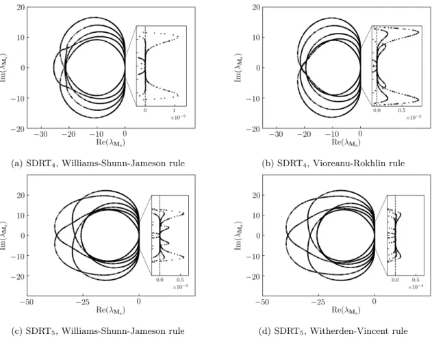
The spectrum of the spatial SDRT operator is computed for p ∈J4, 6K using Fourier analysis for different implementations (i.e. different interior FP locations) for κ ∈ [−π, π], ϑ ∈ [0, 2π], θ = 0 and µ = π/2. The SP location is set to the Williams-Shunn-Jameson quadrature points [65]. Values of max(Re(λMz)) are
displayed in Table 1 for each SDRT implementation based on interior FP locations taken as points of quadrature rules presented before. The first observation is that all SDRT implementations show positive values of max(Re(λMz)), indicating that the spatial discretization is unstable. One can then note that only
two quadrature rules are appropriated for both p = 4, p = 5 and p = 6: the Williams-Shunn-Jameson and the Vioreanu-Rokhlin. For the three polynomial degrees p, the use of the WSJ quadrature rule as the interior FP leads to smaller values of max(Re(λMz)) compared to the Vioreanu-Rokhlin quadrature rule. For the
SDRT5 scheme, two of the quadrature rules (Laursen-Gellert and Papanicolopulos) lead to very high values
of max(Re(λMz)), whereas the smaller value is given by the Witherden-Vincent quadrature rule. For the
Quadrature rule SDRT4 SDRT5 SDRT6 Williams-Shunn-Jameson [65] 1.11 ⋅ 10−5 5.85 ⋅ 10−5 2.87 ⋅ 10−3 Vioreanu-Rokhlin [64] 8.29 ⋅ 10−3 1.75 ⋅ 10−2 2.92 ⋅ 10−2 Laursen-Gellert [60] - >1012 9.82 ⋅ 10−1 Witherden-Vincent [68] - 1.31 ⋅ 10−5 -Xiao-Gimbutas [63] - 7.33 ⋅ 10−2 -Papanicolopulos [69] - >1012
-Table 1: Values of max(Re(λMz))for θ = 0 using different quadrature rules as the interior FP locations
Spectra of unstable discretizations are plotted in Fig. 3 for SDRT4 using Williams-Shunn-Jameson
(Fig. 3a) and Vioreanu-Rokhlin (Fig. 3b) quadrature rules and for SDRT5 using Williams-Shunn-Jameson
(Fig. 3c) and Witherden-Vincent (Fig. 3d). A closer view on each spectra allows one to clearly see the positive eigenvalues real part of the spatial operator Mz for θ = 0.
(a) SDRT4, Williams-Shunn-Jameson rule (b) SDRT4, Vioreanu-Rokhlin rule
(c) SDRT5, Williams-Shunn-Jameson rule (d) SDRT5, Witherden-Vincent rule
Figure 3: Fourier footprint of the SDRT4 and SDRT5 spatial discretizations on triangles for θ = 0 using
4
Determination of Stable Formulations through an Optimization
Process
4.1
Optimization Algorithm
To determine spatially stable SDRT formulations for orders of accuracy higher than four, the Fourier analysis is used in an optimization problem. The function to minimize is the maximum of the real part of the matrix Mz eigenvalues and the optimization parameters are the interior FP locations. The optimization process
solves the problem of minimizing a function locally using a gradient descent method called the L-BFGS-B method from the SciPy library [70]. The L-BFGS-B algorithm is part of the Broyden-Fletcher-Goldfarb-Shanno (BFGS) algorithms, which are iterative methods for solving unconstrained nonlinear optimization problems. The descent direction is determined by preconditioning the gradient with curvature information. The full algorithm is detailed by Algorithm 1 for the SDRT4scheme. First, the constant parameters are
settled: the polynomial degree p is set to 4, the SP location is set to the position given by the 15-points Williams-Shunn-Jameson quadrature rule and the position of FP located on edges is set to Gauss-Chebyshev points. The interior FP coordinates are then parametrized by a set of coefficients to ensure symmetry. The parametrization is given in D for p ∈J4, 5K. The initial interior FP location, stored in x0, is chosen as the 10-points Williams-Shunn-Jameson quadrature rule, expressed using the optimization parameters. Bounds are given to ensure that all interior FP are included in the triangle. The optimization is then run: the scipy.optimize.minimize function based on the L-BFGS-B method called the function MAIN, using x0 as the initial interior FP location and taking bounds into account.
The function MAIN returns the maximum of all eigenvalues real part of the matrix Mz. The interior FP
coordinates are first computed based on the optimization parameters, which allows to compute the transfer matrix T and the differentiation matrix D. The matrix Mz is computed for:
• the advection angle θ ∈ [0, π], ∆θ = π/8, • the grid frequency κ ∈ [0, π]∆κ = π/32,
• the harmonic plane orientation ϑ ∈ [0, π], ∆ϑ = π/8, • the skew angle µ = π/2.
Finally, the maximum of the real part of all the eigenvalues of Mz, denoted rm, is returned and will be
Algorithm 1Fourier analysis optimization algorithm on triangles for SDRT4
Constants p ←4
SP location: ξSP1∶15←WSJ 15-points rule
Edge FP location: ξF P1∶5 ←Gauss-Chebyshev points ▷Edge 1
ξF P6∶10←Gauss-Chebyshev points ▷Edge 2 ξF P11∶15← Gauss-Chebyshev points ▷Edge 3 Optimization Parameters α1=0.333333333333333, α2=0.055564052669793 β1=0.365789252254277, γ1=0.112639085608754 β2=0.704466288264107, γ2=0.281977603613669 ▷ WSJ 10-points rule β3=0.929744459481616, γ3=0.169338518004915 β4=0.944435947330207, γ4=0.416653920995311 x0 = (α1, α2, β1, β2, β3, β4, γ1, γ2, γ3, γ4) Bounds = (α1, α2∈]0, 0.5[, β1, β2, β3, β4, γ1, γ2, γ3, γ4∈]0, 1[) Optimization Process
call scipy.optimize.minimize(MAIN, x0, Bounds, method=’L-BFGS-B’)
function main ξ16= (β4/2 + γ4, β4/2 − γ4), ξ17= (β1/2 + γ1, β1/2 − γ1) ξ18= (β1/2 − γ1, β1/2 + γ1), ξ19= (α2, α2) ξ20= (β3/2 − γ3, β3/2 + γ3), ξ21= (β2/2 + γ2, β2/2 − γ2) ξ22= (β4/2 − γ4, β4/2 + γ4), ξ23= (β3/2 + γ3, β3/2 − γ3) ξ24= (α1, α1), ξ25= (β2/2 − γ2, β2/2 + γ2) ξF P26∶35=ξF P16∶25
Compute Transfer Matrix T Compute Differentiation Matrix D
for µ = π/2 do ▷ Skew angle
for ϑ ∈ [0, π], ∆ϑ = π/8 do ▷ Harmonic plane orientation for θ ∈ [0, π], ∆θ = π/8 do ▷Advection angle
Compute M0,0, M−1,0, M+1,0, M0,−1, M0,+1
for κ ∈ [0, π], ∆κ = π/32 do ▷Grid frequency Compute Mz using:
Mz= −[M0,0+M−1,0exp ( − Iκ cos ϑ) +M+1,0exp (Iκ cos ϑ)
+M0,−1exp ( − Iκ(cos µ cos ϑ + sin µ sin ϑ)) +M0,+1exp (Iκ(cos µ cos ϑ + sin µ sin ϑ))] Compute max(Re(λMz)) rm = max(rm, max(Re(λMz))) end for end for end for end for returnrm end function
4.2
Spatially Stable SDRT
4and SDRT
5Formulations
4.2.1 Sets of Interior Flux Points
The optimization process based on the L-BFGS-B algorithm was able to determined spatially stable SDRT4
and SDRT5 formulations. Parameters leading to stable formulations are given in Table 2. It should be
underlined that there is no proof of the uniqueness of the set of interior FP leading to stable SDRT for-mulations. The interior FP coordinates leading to stable SDRT formulations are actually very close to the coordinates given by the Williams-Shunn-Jameson quadrature rule. This was an expected result due to the local optimization process that looks for a stable formulation close from the initial guess. Both sets of points are compared in Fig. 4. However, as shown in the next section, stability conclusions are quite different.
SDRT4 α1 0.333662142203650535776660035481 − α2 0.055020323277656914273681110217 − β1, γ1 0.365059009419342217483972490299 0.108257446975053225890484043248 β2, γ2 0.708381218412728386191190566024 0.280178103202688211226245584839 β3, γ3 0.926728983000098982536485436867 0.171864737328125433135639354987 β4, γ4 0.944808774978659671184288981749 0.417031665213158209137844778525 SDRT5 α1 0.036016387170921100591147734349 − α2 0.242883711163165288970944288849 − α3 0.473302808618061232603935195584 − β1, γ1 0.248653272121269142136412710897 0.075375559486304394285482999294 β2, γ2 0.526107168266496727504488717386 0.209538637206618832964366561100 β3, γ3 0.757463072390737846006913969177 0.136207500360293581875836821382 β4, γ4 0.800198118640534361567517862568 0.351271727643196640666900520955 β5, γ5 0.950995381781191140291298324883 0.275567788676654157331569194866 β6, γ6 0.963872542677753130213602617005 0.446716481619443550599157788383
Table 2: Coordinate parameters of interior FP determined using the optimization process on Fourier analysis
(a) SDRT4 (b) SDRT5
Figure 4: Sets of FP determined using the optimization process on Fourier analysis compared to Williams-Shunn-Jameson sets
4.2.2 Fourier Analysis of the Spatial Discretization
The Fourier analysis of the spatial SDRT discretization based on the interior FP determined by the opti-mization process is conducted. The spectrum of Mz is first computed for:
• the advection angle θ = 0, • the grid frequency κ ∈ [−π, π],
• the harmonic plane orientation ϑ ∈ [0, 2π], • the skew angle µ = π/2.
These conditions are exactly the same as the ones used in Sec. 3.4, where the SDRT discretization was proven as unstable for p = 4 and p = 5. The spectrum of Mz using the interior FP determined by the optimization
process is displayed in Fig. 5a for SDRT4 and in Fig. 5b for SDRT5. For each order, the Fourier footprint
obtained using the SDRT is similar to the one obtained using interior FP located at quadrature rules points (Fig. 3a and Fig. 3c) except that positive eigenvalues have been pushed to the negative side, leading to stable formulations. Spectra are then computed in the general case, i.e. for θ ∈ [0, π], κ ∈ [−π, π], ϑ ∈ [0, 2π] and µ ∈ [π/2, π/3, π/4]. Corresponding Fourier footprints are shown in Fig. 5c for SDRT4 and in Fig. 5d
for SDRT5. From these spectra, the linear stability of the SDRT spatial discretization is clearly established
since the real part of all eigenvalues is negative.
(a) SDRT4, θ = 0 (b) SDRT5, θ = 0
(c) SDRT4, General Case (d) SDRT5, General Case
4.2.3 Fourier Analysis of the Coupled Time-Space Discretization
To investigate the linear stability of the coupled time-space discretization, the semi-discretized form needs to be integrated in time. Considering a differential equation:
∂u
∂t =R(u), (55)
a general m-stage Runge-Kutta (RK) method for Eq. (55) can be written as in [71]: ⎧ ⎪ ⎪ ⎪ ⎪ ⎨ ⎪ ⎪ ⎪ ⎪ ⎩ u(l) = l−1 ∑ k=0 (αlku(k)+∆tβlkR(u(k))), l =1, ..., m, u(0) =u(n), u(m)=u(n+1), (56)
where, in the case of Eq. (49), R(u(k)) = −∇ ⋅f (u(k)). In this paper, the time-integration scheme used is the SSP3s3o of Gottlieb and Shu, which is part of the family of Total Variation Diminishing (TVD) time discretization [71], later called Strong Stability Preserving (SSP) schemes [72]. The nonlinear stability property of these methods makes them particularly appropriated for the time-integration of hyperbolic partial differential equations.
The semi-discretized matrix form containing the planar harmonic wave given by Eq. (54) integrated in time using Eq. (56) is:
⎧ ⎪ ⎪ ⎪ ⎪ ⎨ ⎪ ⎪ ⎪ ⎪ ⎩ G(l) = ( l−1 ∑ k=0 (αlkI + νβlkMz))G(k), l =1, ..., m, G(0) =I, U˜(n+1)=G ˜U(n), (57)
where G = G(m)and ν is the CFL number defined by: ν =∣∣c∣∣∆t
∆x . (58)
The stability condition on the coupled time-space discretization is thus obtained by requiring that the amplitude of any harmonic does not grow in time, i.e.:
∣G∣ = ∣U˜
(n+1)
˜
U(n) ∣ ≤1. (59)
In other words, to ensure a stable discretization, the spectral radius of the matrix G, denoted ρGshould be
lower than 1, meaning that all the eigenvalues λG should be in the unit circle of the complex plane. The
transfer matrix G between time steps n and n + 1 is the amplification factor (or the Fourier symbol) of the full discretization.
The linear stability of the coupled time-space discretization is now analyzed through the study of the spectral radius of the amplification factor ρG. The following parameters are considered in the study:
• θ ∈ [0, 2π], ∆θ = π/8, • κ ∈ [−π, π], ∆κ = π/32, • ϑ ∈ [0, 2π], ∆ϑ = π/8, • µ = (π/2, π/3, π/4).
The CFL stability limits are given for those parameters in Table 3. Note that values are associated with the classical definition of the CFL number given by Eq. (58). To compare CFL numbers used in high-order discontinuous methods with classical methods (like Finite Volume, Finite Element or Finite Difference), one can introduced an equivalent CFL number ˆνdefined as ˆν = (p +1)ν [46]. This equivalent CFL number makes sense in the one-dimensional case since (p + 1) is a length scale corresponding to the mean distance between two adjacent SP. However, this definition is not necessarily the most adequate one on triangles, as shown by Chalmers and Krivodonova [73] for the DG method. To the authors’ knowledge, there is no consensus on the definition on an equivalent CFL number for high-order discontinuous methods on simplex cells. The classical CFL definition is thus preferred here.
θ =0 θ = π/8 θ = π/4 θ ∈ [0, 2π], ∆θ = π/8 SDRT4 0.097 0.081 0.075 0.075
SDRT5 0.065 0.057 0.054 0.054
Table 3: CFL stability limits ν for SDRT schemes on triangles coupled with the SSP3s3o temporal schemes
5
Numerical Experiments
5.1
Convection of an isentropic vortex
A nonlinear case is now studied by considering the two-dimensional Euler equations: ∂u ∂t + ∂f ∂x+ ∂g ∂y =0, in Ω × [0, tf], (60) where u, f and g are given by:
u = ⎛ ⎜ ⎜ ⎜ ⎝ ρ ρU ρV E ⎞ ⎟ ⎟ ⎟ ⎠ , f = ⎛ ⎜ ⎜ ⎜ ⎝ ρU ρU2 +P ρU V U (E + P ) ⎞ ⎟ ⎟ ⎟ ⎠ , g = ⎛ ⎜ ⎜ ⎜ ⎝ ρV ρV U ρV2 +P V (E + P ) ⎞ ⎟ ⎟ ⎟ ⎠ . (61)
In Eq. (61), ρ is the density, U (respectively V ) is the velocity component in the x (respectively y) direction, E is the total energy and P is the pressure determined from the following equation of state:
P = (γ −1) (E −1 2ρ(U
2
+V2)), (62) where the constant ratio of specific heats γ is equal to 1.4 for air.
To assess the SDRT scheme accuracy and capability to preserve vorticity in an unsteady inviscid flow, the convection of an isentropic vortex (COVO) test case from the International Workshop on High-Order CFD Methods [74] is studied. An isentropic vortex is transported by an inviscid uniform flow defined by P∞ = 105Pa, T∞ = 300 K, M∞ = U∞/
√
γRgasT∞ = 0.5. The fluid is assumed to be a perfect gas, with a constant ratio of specific heats γ = 1.4. An isentropic vortex of characteristic radius R = 0.005 m and strength β = 0.2 is added to this mean flow around the point of coordinates (Xc, Yc) = (0.05, 0.05) through perturbation in U , V and the temperature T . The computation is thus initialized by the local velocity components U0 and V0 as well as temperature T0:
U0=U∞(1 − β (y − Yc) R exp (−r 2 /2)) , (63) V0=U∞β (x − Xc) R exp (−r 2/2), (64) T0=T∞− U∞2β2 2Rgas (γ −1) γ exp (−r 2), (65) where r = √ (x − Xc)2+ (y − Yc)2 R . (66)
Since the vortex is isentropic, the density can be computed using:
ρ0=ρ∞( T0 T∞) 1 γ−1 , (67)
where ρ∞ = P∞
RgasT∞. Euler equations are solved on the computational domain Ω = [0, L]
2 where L =
0.1 m. Translational periodic boundary conditions are imposed for the left/right and top/bottom boundaries respectively. The SSP3s3o scheme introduced for the coupled time-space analysis is considered for the simulations. The time step is chosen sufficiently small so that the error from the time discretization is negligible compared to the spatial discretization error by setting the CFL number to 10−2. At interfaces, Roe’s Riemann solver [75] was used to compute the numerical flux. Figure 6 gives the initial solution by showing ρV contours (product of the density ρ and the y-velocity V ) on a regular mesh composed of 2N2
triangles using a SDRT5scheme.
Figure 6: Initialization of the COVO test case using SDRT5and N = 20 on a triangular grid
A mesh refinement study is performed using regular triangular and hybrid grids of different size after 5 periods. To generate hybrid grids, the left part of the computational domain (x ∈ [0, 0.05]) is meshed using quadrilateral elements whereas the right part (x ∈ [0.05, 0.1]) is meshed with triangles. The mesh is composed of 1
2N
2 quadrilaterals and N2 triangles. The numerical scheme used for quadrilateral cells is the
standard SD method based on the interior FP located at the zeros of the corresponding Legendre polyno-mials. The very same polynomial degree is used for both triangular and quadrilateral elements.
To verify the order of accuracy of the SDRT scheme, the L2 error on the density can be computed at
each period on the domain as:
L2= ¿ Á Á À ∫Ω(ρh0−ρnum) 2 dΩ ∫ΩdΩ , (68)
where ρh0 is the polynomial approximation of the initial solution ρ0.
In Eq. (68), the integral on the top can be expressed as the following sum on each cell:
∫ Ω (ρh0−ρnum) 2 dΩ = N ∑ i=1 ∫ Ωi (ρ(i)h 0 −ρ (i) num) 2 dΩ, (69)
using a quadrature rule such that: N ∑ i=1 ∫ Ωi (ρ(i)h 0 −ρ (i) num) 2 dΩ = N ∑ i=1 Nq ∑ j=1
A ∣J(i,j)∣ωj(ρ(i)h0(ξj) −ρ(i)num(ξj))) 2
, (70)
where A is the reference element area (A = 1 for a quadrilateral element and A = 1/2 for a triangular element), ∣J(i,j)∣ is the Jacobian determinant at the j-th integration point of the i-th cell and Nq is the number of
quadrature points. The quadrature points are located at ξj and associated with the weight ωj. Since ρh0
and ρnum are polynomials of degree p, the term (ρ(i)h0 −ρ(i)num)
2
should be approximated using a quadrature of degree 2p. On triangles, the integration is carried out using the 175-points symmetric quadrature given by Wandzura and Xiao [76], which can be used up to degree 30. On quadrilaterals, the integration is per-formed using the tensor product of two 1D integration at SP, with the appropriate Gauss-Chebyshev weights. The L2norm of the density error is plotted in Fig. 7 after 5 time-periods and compared with the expected
order slope. For both triangular and hybrid grids, the expected order of accuracy p + 1 is retrieved. The precise overall order of accuracy, computed using a least squares polynomial fit of degree one, is given in Table 4)
(a) Triangular Grids (b) Hybrid Grids
Figure 7: L2 error and theoretical order of accuracy slopes for the COVO test case after 5 periods
Scheme Order of accuracy SDRT2 3.03
SDRT3 4.02
SDRT4 4.98
SDRT5 6.19
(a) Triangular Grids
Scheme Order of accuracy SD/SDRT2 3.00
SD/SDRT3 4.02
SD/SDRT4 5.05
SD/SDRT5 6.09
(b) Hybrid Grids Table 4: Overall accuracy orders for the COVO test case after 5 periods
5.2
Viscous flow over an NACA0012 airfoil
This test case aims to validate the method for the computation of viscous flow with a high-order triangular curved boundary representation. The compressible Navier-Stokes equations are solved and a laminar viscous flow over the NACA0012 airfoil is considered. The computational setup is defined by the angle of attack α, the Mach number M∞ and the Reynolds number Re = ρ∞U∞C/µd∞, where C is the airfoil chord. Three
different laminar flow conditions chosen from the NASA technical report [77] are considered: • Case A: Symmetric subsonic flow, M∞=0.5, α = 0°, Re = 5000,
• Case B: Asymmetric subsonic flow, M∞=0.5, α = 2°, Re = 5000, • Case C: Transonic flow, M∞=0.8, α = 10°, Re = 500.
The NACA0012 airfoil equation used is:
y = ±0.6 (0.2969√x −0.1260x − 0.3516x2
+0.2843x3−0.1036x4), (71) so the trailing edge has a zero thickness. At the airfoil, a no-slip adiabatic wall condition is imposed. To avoid spurious reflections on the boundary conditions, the farfield boundary is located 50 chords away from the airfoil. On the farfield boundary, pressure and temperature are imposed at P∞=101325Pa and T∞=293.15K and the velocity is imposed depending on the Mach number. Interface flux is then obtained by applying the approximated Riemann solver at the interface using the prescribed state outside and the extrapolated internal state. The computational domain is meshed with a C-type topology and has a total number of 2407 quadratic triangular elements (with 62 cells on the airfoil). A close view of the resulting mesh is shown in Fig. 8. Solutions are time-integrated using the SSP3s3o temporal scheme and the convection flux is Roe’s scheme. Results are presented for SDRT schemes from the third- to the sixth-order (p ∈J2, 5K). The CFL number is chosen based on the maximum one affordable using p = 5, i.e. ν = 0.05. The visualization process on triangular grids is done by extrapolating the solution at SP to high-order Lagrange elements nodes. 5.2.1 Thorough Analysis of Case C
Results obtained for Case C are first presented in details since the transonic flow can be considered as the ’most critical’ test case. For the subsonic flows (Case A and B), briefer results will be given in the next section. To monitor the computation convergence, the L2 norm of the residual on the density between iteration
nand n + 1 is computed using:
∣∣Res∣∣2= ¿ Á Á À ∫Ω(ρn+1−ρn) 2 dΩ ∫ΩdΩ . (72)
Integration is performed using the 175-points symmetric quadrature given by Wandzura and Xiao [76]. The decay of the residual against number of iteration for SDRTp schemes, p ∈J2, 5K, is shown for the transonic Case C in Fig. 9. Despite the use of an explicit time-integration scheme, a very good convergence is obtained.
−0.5 0.0 0.5 1.0 1.5 2.0 x/C −0.8 −0.6 −0.4 −0.2 0.0 0.2 0.4 0.6 0.8 y /C
Figure 8: Close view of the unstructured mesh around a NACA0012airfoil 106 107 108 Iteration number 10−18 10−16 10−14 10−12 10−10 10−8 || Res ||2 SDRT2 SDRT3 SDRT4 SDRT5
Figure 9: Convergence of the residual for the tran-sonic viscous flow over a NACA0012 airfoil
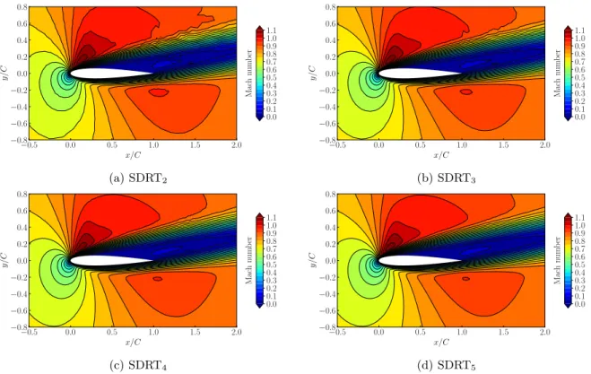
Fig. 10 shows the Mach contours obtained with SDRT schemes of 3rd to 6thorder of accuracy for Case
C. The flow is accelerated at the airfoil upper surface and create a small supersonic zone (M > 1). However, as expected for this case, there is no shock wave developing. As the degree of the polynomial reconstruction increases, the solution becomes smoother and thus more accurate. For SDRT2and SDRT3schemes (Fig. 10a,
10b), discontinuous contour lines can be observed. Those discontinuities are induced by the visualization process, which is done independently on each triangular element, leading to different solution values at cell interfaces, and express a low resolution. The Mach contours given by the SDRT4 and SDRT5 schemes
(Fig. 10c, 10d) show continuous lines for most of the domain. The remaining discontinuities located around the position (x/C, y/C) = (1.4, 0.4) are due to the fact that the mesh used is refined for the wake given with an angle of attack α = 0o. Apart from this region, the Mach contours obtained show that the 5th and 6th
order SDRT schemes converge to the same solution.
−0.5 0.0 0.5 1.0 1.5 2.0 x/C −0.8 −0.6 −0.4 −0.2 0.0 0.2 0.4 0.6 0.8 y /C 0.0 0.1 0.2 0.3 0.4 0.5 0.6 0.7 0.8 0.9 1.0 1.1 Mac h num b er (a) SDRT2 −0.5 0.0 0.5 1.0 1.5 2.0 x/C −0.8 −0.6 −0.4 −0.2 0.0 0.2 0.4 0.6 0.8 y /C 0.0 0.1 0.2 0.3 0.4 0.5 0.6 0.7 0.8 0.9 1.0 1.1 Mac h num b er (b) SDRT3 −0.5 0.0 0.5 1.0 1.5 2.0 x/C −0.8 −0.6 −0.4 −0.2 0.0 0.2 0.4 0.6 0.8 y /C 0.0 0.1 0.2 0.3 0.4 0.5 0.6 0.7 0.8 0.9 1.0 1.1 Mac h num b er (c) SDRT4 −0.5 0.0 0.5 1.0 1.5 2.0 x/C −0.8 −0.6 −0.4 −0.2 0.0 0.2 0.4 0.6 0.8 y /C 0.0 0.1 0.2 0.3 0.4 0.5 0.6 0.7 0.8 0.9 1.0 1.1 Mac h num b er (d) SDRT5
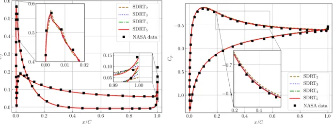
The surface skin-friction coefficient Cf and the surface pressure coefficient Cpdistributions are plotted in
Fig. 11 and Fig. 12. For both coefficients, there is good agreement between the results obtained from SDRTp
schemes and the NASA data [77]. In Fig. 11, a closer view shows that all SDRT schemes were able to capture the maximum value of the surface skin-friction coefficient at the leading edge. Small discontinuities between cells are observed, resulting from the interpolation post-processing step performed independently on each cell. The peak at the leading edge is quite accurately represented. A difference with the NASA data can be noticed at the trailing edge, where SDRT schemes did not manage to capture the maximum values due to low mesh refinement. A close view indicates that the SDRT Cf value gets a bit closer to the reference one
when the order of accuracy increases. The surface pressure coefficient plot (Fig. 12) shows that all SDRTp
schemes lead to excellent agreement with the NASA data, including at leading and trailing edges. As for the first two cases, results converge when the order increases.
Figure 11: Case C: Surface skin-friction coefficient Cf Figure 12: Case C: Surface pressure coefficient Cp
5.2.2 Aerodynamic Coefficients Computation for Three Different Laminar Flow Conditions For each case, aerodynamic coefficients are computed for each SDRT scheme and compared to NASA refer-ence data in Table 5.
For Case A, an additional comparison is made with results obtained using a standard fifth-order SD scheme in [78]. Values of the different coefficients converge as the order of accuracy increases and get closer to the reference data. Results using SDRT4are in excellent agreement with the NASA data using the refined
grid (difference of 0.1%), whereas SDRT5 matches results obtained using the fifth-order SD scheme
(differ-ence of 0.7%). All of the separation point locations predicted by SDRT schemes lies in the interval given by the two references up to the third decimal.
For Case B, the SDRT2 scheme leads to a good prediction of CD (1% of difference), but the surface
skin-friction and pressure coefficients are not accurately determined (∼ 4.5% of difference). For higher-order SDRT schemes, the CD value converges to the NASA reference (13% for SDRT3, 2.8% for SDRT4 and 0.8%
for SDRT5), with close values for (CD)p and (CD)f. The same behavior is observed for the separation point location, even if it is slightly overestimated (2.8% for p = 5).
Finally, for Case C, results for the total drag coefficient are in excellent agreement with the NASA reference, with a difference of < 2% for all schemes. For p > 2, all coefficients are converged up to the third decimal. The location of the separation point is slightly smaller than the reference ones but remains in good agreement.
DoF Number CD (CD)p (CD)f xsep/C Case A SDRT2 14, 442 0.0583644 0.0220679 0.0362965 0.809 SDRT3 24, 070 0.0573619 0.0239848 0.0333771 0.808 SDRT4 36, 105 0.0554990 0.0225962 0.0329028 0.810 SDRT5 50, 547 0.0543702 0.0218255 0.0325447 0.814 NASA [77] 1024 × 512 (524, 288) 0.0555743 0.0227887 0.0327855 0.808 Fifth-order SD [78] 360 × 120 (43, 200) 0.05476 0.02225 0.03251 0.814 Case B SDRT2 14, 442 0.0574735 0.0233123 0.0341613 0.584 SDRT3 24, 070 0.0644525 0.0298255 0.0346270 0.580 SDRT4 36, 105 0.0584788 0.0252599 0.0332190 0.579 SDRT5 50, 547 0.0573627 0.0245549 0.0328078 0.577 NASA [77] 1024 × 512 (524, 288) 0.0568914 0.0243173 0.0325741 0.561 Case C SDRT2 14, 442 0.272783 0.148275 0.124508 0.357 SDRT3 24, 070 0.270953 0.147087 0.123867 0.356 SDRT4 36, 105 0.270255 0.146632 0.123622 0.355 SDRT5 50, 547 0.270224 0.146715 0.123509 0.355 NASA [77] 1024 × 512 (524, 288) 0.275155 0.147544 0.127611 0.362 Table 5: Comparison of drag coefficients and separation point location
5.3
Viscous flow around a circular cylinder
This test case aims to validate the method for the computation of viscous flow using 2D hybrid mesh. A steady laminar viscous flow at Re = 20 around a cylinder is considered. The Mach number is M∞=0.1 and the Reynolds number is defined by Re = ρ∞U∞d/µd∞, where the dynamic viscosity is µd∞=1.853 ⋅ 10−3Pa s, and the cylinder diameter is d = 1 m. The density ρ∞ and the velocity U∞can be deduced from the temperature T =300K and the constant ratio of specific heats γ = 1.4. The cylinder is placed in a rectangular domain. The farfield boundaries are located 10 diameters away from the cylinder in the upstream, upward and downward directions and 30 diameters away in the downstream direction. A hybrid mesh of 3427 elements is used, with 196 quadrilateral elements near the cylinder and 3231 triangles in the rest of the domain. A close view of the mesh is provided in Fig. 13. On the farfield boundary, the pressure, temperature and velocity are settled. At the cylinder surface, a no-slip isothermal wall condition is imposed. On quadrilateral elements, the standard SD method based on the interior FP located at the zeros of the corresponding Legendre polynomials is used. The same polynomial degree is used for both triangular and quadrilateral elements. Roe’s Riemann solver is used to compute flux at interface flux points and the CFL number is set to 0.05 (the maximum one affordable using p = 5). The computation convergence is monitored by computing the L2 norm of the residual on the
density between iteration n and n + 1 using:
∣∣Res∣∣2= ¿ Á Á À ∫Ω(ρn+1−ρn) 2 dΩ ∫ΩdΩ . (73)
Integration is performed using the 175-points symmetric quadrature given by Wandzura and Xiao [76]. The decay of the residual against number of iteration for SD/SDRTp schemes, p ∈J2, 5K, is shown in Fig. 14. As for NACA test cases, computations are very well converged.
−2 0 2 4 x −3 −2 −1 0 1 2 3 y
Figure 13: Close view of the hybrid mesh for the viscous flow around a cylinder
Figure 14: Convergence of the residual for the viscous flow around circular cylinder
Figure 15 shows the normalized x-velocity contours and streamlines around the cylinder obtained using a SD/SDRT5 scheme. Streamlines show a recirculation zone within the wake of the cylinder where two
vortices are generated.
(a) Normalizedx-velocity contours (b) Close view of streamlines and normalizedx-velocity contours Figure 15: Normalized x-velocity contours and streamlines around the cylinder using a SD/SDRT5scheme
Values of the drag coefficients as well as the separation angle θsep and the normalized reattachment
length L/d obtained using SD/SDRT schemes are compared with different reference values in Table 6. Values presented are computed after applying a Savitzky-Golay filter; however, note that the maximum difference between values on all coefficients obtained with and without the filter is around 0.2%. Reference results [79, 80, 81] are based on finite difference approximation and Cartesian grids. Compared to data from Dennis and Chang, the SD/SDRT scheme overestimates drag coefficients values. This overestimation could be due to the fact that linear quadrilateral elements were used. A mesh composed of quadratic elements could lead to better results. Additionally, using a no-slip adiabatic wall condition at the cylinder surface instead of an isothermal wall condition could be more appropriate. However, compared to other reference data, SD/SDRT schemes lead to a proper estimation of drag coefficients, separation angle and reattachment length.