Capitalisation of government support in agricultural land prices: what do we know?

HAL Id: hal-02285614

https://hal.archives-ouvertes.fr/hal-02285614

Submitted on 12 Sep 2019

HAL is a multi-disciplinary open access archive for the deposit and dissemination of sci-entific research documents, whether they are pub-lished or not. The documents may come from

L’archive ouverte pluridisciplinaire HAL, est destinée au dépôt et à la diffusion de documents scientifiques de niveau recherche, publiés ou non, émanant des établissements d’enseignement et de

Capitalisation of government support in agricultural

land prices: what do we know?

Laure Latruffe, Chantal Le Mouël

To cite this version:

Laure Latruffe, Chantal Le Mouël. Capitalisation of government support in agricultural land prices: what do we know?. [University works] Inconnu. 2007, 39 p. �hal-02285614�

Institut National de la recherche Agronomique Unité d'Economie et Sociologie Rurales

4 Allée Adolphe Bobierre, CS 61103 F 35011 Rennes Cedex

Tél. (33) 02 23 48 53 82/53 88 - Fax (33) 02 23 48 53 80

http://www.rennes.inra.fr/economie/index.htm

Capitalisation of government support in agricultural land prices:

What do we know?

Laure Latruffe and Chantal Le Mouël

September 2007 Working Paper 07-04

Capitalisation of government support in agricultural land prices:

What do we know?

Laure Latruffe INRA – Unité ESR Rennes

Chantal Le Mouël INRA – Unité ESR Rennes

Corresponding address: Laure LATRUFFE INRA – Unité ESR

4 Allée Bobierre, CS 61103 35011 Rennes Cedex, France

Email: Laure.Latruffe@rennes.inra.fr Phone: 0033 2 23 48 53 93

3 Capitalisation of government support in agricultural land prices:

What do we know? Abstract

The objective of this article is to provide an overview of existing literature, both theoretically and empirically, on the extent to which agricultural subsidies do translate into higher land values and rents and finally benefit landowners instead of agricultural producers. Our review shows that agricultural support policy instruments contribute to increase the rental price of farmland, and that the extent of this increase closely depends on the level of the supply price elasticity of farmland relative to those of other factors/inputs on the one hand, and on the range of the possibilities of factor/input substitution in agricultural production on the other hand. The empirical literature shows that land prices and rents have a significant positive response to government support, consistently less than 1. Such inelastic response is thought to reflect the uncertain future of the farm programs. And in general, studies have indicated that land prices are more responsive to government-based returns than to market-based returns. Keywords: farmland, price, support, capitalisation

JEL Classification: Q18, Q15

Capitalisation du soutien public dans les prix des terres agricoles : Que sait-on exactement ?

Résumé

L’article propose une revue de la littérature théorique et empirique sur la question de la capitalisation des subventions versées à l’agriculture dans les prix et les loyers des terres agricoles et, par suite, de l’éventuel transfert de ces subventions des producteurs agricoles, à qui elles sont destinées, vers les propriétaires terriens. Notre revue montre que les instruments de soutien à l’agriculture contribuent à accroître le prix de location des terres agricoles. L’ampleur de cette augmentation dépend étroitement i) du niveau de l’élasticité prix de l’offre de terre agricole par rapport à celle des autres facteurs de production, ii) des possibilités de substitution entre facteurs de production au sein de la technologie de production agricole. La littérature empirique suggère quant à elle que les prix de vente et de location des terres agricoles répondent significativement et positivement au soutien public, et que l’élasticité de cette réponse est inférieure à 1. L’inélasticité de la réponse des prix des terres agricoles au

soutien public octroyé à l’agriculture pourrait refléter le fait que l’avenir des programmes de soutien agricoles est perçu comme incertain par les opérateurs des marchés. En outre, généralement les études existantes indiquent que les prix des terres agricoles répondent plus fortement à la composante soutien public, qu’à la composante gain issu de l’activité de production (ventes des produits).

Mots-clés : terre agricole, prix, soutien, capitalisation Classification JEL : Q18, Q15

5 Capitalisation of government support in agricultural land prices:

What do we know?

1. Introduction

A central purpose of agricultural policies in industrialised countries is to support farmers’ income. Whether agricultural support actually benefits farmers however is an open question. Agricultural support policies raise farmers’ gross income and then contribute to increase returns to resources that individual farmers use. As a consequence, agricultural support policies contribute to increase the market prices of these resources and ultimately benefit the owners of these resources. Hence, whether agricultural support benefits farmers closely depends on whether farmers own the resources they use in production.

Among agricultural primary factors of production (land, family labour and capital), land has been paid higher attention regarding this issue for at least two reasons. Firstly, in many industrialised countries, a substantial share of farmland is rented, sometimes from other farmers but also commonly from non-farmer landlords. Secondly, an increasing number of government payments are tied to farmland. Hence the question of the extent to which agricultural subsidies do translate into higher land values and rents and finally benefit landowners, is a critical issue.

Concern over the capture of agricultural policy benefits by the landowners is not new. And the question of the capitalisation of support into farmland values and rents has a long tradition in Agricultural Economics. The objective of this article is to provide an overview of existing literature, both theoretically and empirically, on that issue.

The article is structured as follows. The next section reviews the main insights that can be drawn from the theory about how agricultural support may affect farmland values and rents and what are the key assumptions and parameters regarding this issue. The third section reviews empirical evidence about the extent to which agricultural support affects farmland values and rents. The final section concludes.

2. Agricultural support does affect farmland markets and prices: Insights from the theory

By which mechanisms agricultural support does affect farmland markets and prices? What are the main assumptions and parameters that play a key role as regards the extent of the impact

of agricultural support on farmland markets and prices? Who finally benefit from agricultural support?

This section synthesises the main insights that can be drawn from the theory regarding these three questions. We focus on the relationships between agricultural support and farmland rental markets and prices. It is commonly assumed in existing studies that the buying and selling prices of farmland can be adequately approximated by the discounted sum of future rental prices, so that a prediction about the direction of the rental prices is equivalent to a prediction about the direction of the buying and selling prices. As a result most theoretical work has focused on the rental price of farmland. We concentrate on two types of policy instruments: output price support and land subsidy. These two instruments have been selected because they reflect the evolution of agricultural policies in most industrialised countries over the last decade, where output price support has been progressively replaced by direct payments linked to production factors, especially land.

The main insights that can be drawn from theory on the effects of output price support on farmland rental markets and prices are first reviewed. Then, we focus on what we know from the theory about the effects of factor (especially land) subsidies. In both cases, using very simple frameworks, the main mechanisms that underlie the effects of policy instruments are described by the mean of a graphical analysis.

2.1. Output price support and farmland rental markets and prices

One paper extensively cited in the existing literature is Floyd (1965). This seminal paper shows, using a rather simple analytical model, that: i) output price support affects the prices of production factors1; ii) the extent of the impact of output price support on factor prices closely depends on the elasticities of supply of factors (that is the extent of factor mobility within the economy) and on agricultural production technology (that is, specifically, the extent of factor substitution possibilities); iii) output control programs (through production quota or acreage restriction) modify the effect of output price support on factor prices, either by creating a new fixed production factor (production rights) in the case of quota, or by changing the opportunity cost of land in the case of acreage restriction.

A number of papers have re-examined in alternative ways Floyd’s results or extended them by relaxing restrictive hypotheses of Floyd’s model and/or including various alternative policy

1

In this paper the term ‘production factors’ refer to land, family labour and capital, while the term ‘inputs’ designate all other (variable) inputs such as hired labour, energy, fertiliser, pesticides, etc.

7 instruments in order to compare their respective effects (e.g., Gardner, 1987; Hertel, 1989; 1991; Leathers, 1992; Dewbre et al., 2001; Dewbre and Short, 2002; OECD, 2002; Guyomard et al., 2004). Usually however, although analytical results are much more complicated and effects of policy instruments more difficult to disentangle, interpret and sign, main insights from Floyd’s model do remain.

The one output-one factor case: Illustrating the key role of factor supply elasticity

Let’s consider a representative farmer using one factor (which may be land) in quantity l to produce an aggregate agricultural output in quantity y , according to a given production technology (y= f(l)). Figure 1 depicts the domestic output and factor markets in the

considered country. On the output market, D_y(p_y) is the domestic demand while ( , 0)

l y

y p p

S

is the initial domestic supply. Both the domestic demand and supply depend on the domestic output price p . The initial output supply also depends on the initial equilibrium price of the _y

factor 0

l

p . Let’s assume that the considered country is a small country for the output y . Hence, at initial equilibrium, domestic output price is 0

y

p corresponding to the exogenous world price. The representative farmer produces quantity y , which is partly consumed 0 domestically and partly exported. On the factor market, D_l(p_l,p0_y) is the initial domestic derived demand, as a function of the factor price and the initial output price, while S_l(p_l) is the domestic factor supply. On panel 1.b this factor supply is assumed to be perfectly inelastic in quantity l ( l is a specific factor to agriculture), while in panel 1.c it is assumed as 0 perfectly elastic at price p . Let’s assume that the factor is not traded. Hence, in both cases, _l0 at initial equilibrium, domestic demand equals domestic supply at price p and quantity _l0 l . 0 Let’s imagine that the government decides to support the farmer’s income through output price support. Hence the output price increases to p1_y.2 In a first step, this output price increase is an incentive for the farmer to produce more. Other things being equal, the farmer

2

This output price support may be provided through a fixed support price or a fixed (ad-valorem or specific) output subsidy. Such alternative instruments would have different impacts for domestic consumers and in terms of net welfare loss for the considered country but not for the representative farmer, nor on the factor market. As we are only interested in the farmer’s situation in conjunction with the impact of output price support on the factor market, we do not specify which type of instrument is used.

would seek to produce y . However, such an output supply increase would require to use 1 more factor. This factor adjustment requirement is depicted through the shift in the derived

demand curve from ( , 0)

y l l p p D to ( , 1) y l l p p

D on the factor market. At this stage one can

guess the key role of the factor supply elasticity:

- In panel 1.b, as the factor supply is perfectly inelastic (i.e., there is no additional quantity of factor available), this factor demand increase translates into a factor price increase from p to _l0 p . The resulting increase in the marginal cost of y is depicted 1_l on panel 1.a through the shift of the output supply curve from S_y(p_y,p_l0) to

) , ( _y 1_l

y p p

S . Finally, figure 1 shows that, following the induced price adjustment on

the factor market, the final equilibrium output quantity is unchanged at 0

y .

- In panel 1.c, as the factor supply is perfectly elastic (i.e., at price p there is no _l0 restriction on available quantity of the factor), the factor demand increase does not affect the factor price, which remains at p level. Hence, the marginal cost of y is _l0

unchanged. Factor demand and output supply increase simultaneously, to 1

y and l 1 respectively.

Finally, if we consider that the factor in figure 1 is land, this figure illustrates the key role of the land supply price elasticity as regards the effect of output price support on the rental price of land: if this elasticity is very low, output price support is nearly totally “capitalised” in the rental price of land, while if this elasticity is very high, output price support has nearly no effect on the rental price of land. In other words, the lower the land supply price elasticity, the higher the share of output price support “capitalised” in the rental price of land. In that case, if the owner of the factor is the farmer, then the price support policy actually contributes to supporting the farmer’s income. At reverse, if the owner of the factor is not the farmer, but an individual who is outside the agricultural sector, the price support policy completely misses its initial objective since the provided support “leaves” the agricultural sector. Furthermore, by contributing to increase the price of the factor, the price support policy increases the cost of setting-up for future farmers. Finally, not only the price support policy misses its initial target group (the current farmers) but it might also contribute to worsen the situation of future farmers.

Figure 1. Effects of output price support on domestic output and factor markets: the one-factor case 1.a. Output market 1.b. Factor market

(supply perfectly inelastic) y

p

p

_l

p

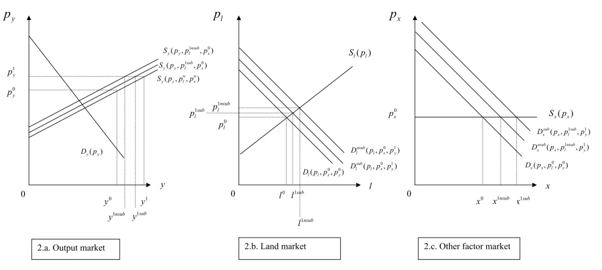
_l y l l 0 y y 0 y p 0 l p 0 l p 0 l l0 1 y p 1 y y 1 l p 1 l ) , ( y 0l y p p S ) , ( 1 l y y p p S ) ( _y y p D ( , ) 0 y l l p p D ) , ( l 0y l p p D ) , ( 1 y l l p p D ( , ) 1 y l l p p D 0 0 0 ) ( _l l p S ) ( _l l p S 1.c. Factor market (supply perfectly elastic)

The one output-two factor case: Illustrating the key role of factor substitution possibilities Let’s assume now that our representative farmer produces an aggregate agricultural output by combining two factors, according to a given production technology (y= f( xl, )). The first factor is land and is used in quantity l . The second factor may be an aggregate of family

labour and capital and is used in quantity x. Figure 2 depicts the domestic output and factor

markets in the considered country.

Notations are similar to the previous case. Panel 2.b describes the domestic land rental market. We assume that the land supply is imperfectly elastic and, consequently, increasing in the rental price of land. Panel 2.c depicts the domestic market of the other factor. The domestic supply of this other factor is assumed to be perfectly elastic in p0_x. On panel 2.a output supply now depends on the output price and on both factor prices. On panels 2.b and 2.c, derived demands of factors also depend on the output price and on both factor prices.

Therefore, ( , 0, 0)

x l y

y p p p

S is the initial output supply curve, while ( , 0, 0)

y x l l p p p D and ) , , ( _{x l}0 0_y x p p p

D are the initial derived demand curves of land and of the other factor

respectively.

All other assumptions adopted in the previous case are still valid here. At initial equilibrium the domestic output price is p0_y, the representative farmer produces quantity _y0_{, using}

quantity l0 of land and quantity x0 of the other factor. The initial rental price of land is p_l0, while the initial price of the other factor is p_x0.

As in the previous case, we assume that, following the implementation of an output price support policy, the output price increases to p1_y. In a first step, this output price increase is an incentive for the farmer to produce more. Other things being equal, the farmer would seek to

produce 1

y . However, such an output supply increase would require to use larger quantities

of factors. This is at this stage that the key role of substitution possibilities between both factors appears.

- Let’s consider first the case where both factors are highly substitutable. As the supply

of factor x is perfectly elastic, an increase in its derived demand would have no impact on its initial equilibrium price. While as the supply of land is imperfectly elastic, an increase in its derived demand would lead the land rental price to increase relative to its initial equilibrium level. Therefore, in the new output price context, the

11 representative farmer who wants to increase his/her output quantity has incentive to change his/her factor quantity ratio in favour of factor x, trying to keep nearly unchanged his/her use of land. Such a situation is represented in panels 2.b and 2.c by the small shift to the right of the derived demand of land (from D_l(p_l,p_x0,p0_y) to

) , , ( _{l x}0 1_y sub l p p p

D ) and the large shift to the right of the derived demand of factor x

(from ( , 0, 0) y l x x p p p D to ( , 1 , 1) y sub l x sub x p p p

D ). Hence, at final equilibrium, the farmer

produces quantity y1sub using quantity l1sub of land and quantity x1sub of the other factor. In this case, factor prices are nearly unchanged (one observes only a slight increase in the rental price of land from p_l0 to sub

l

p1 ) with respect to the initial equilibrium.

- Let’s consider now the situation where land and the other factor are hardly

substitutable. In that case, the representative farmer is more constrained in the adjustment of his/her factor quantity ratio in favour of factor x. This more constrained factor substitution process is illustrated in panels 2.b and 2.c by the shift to the right of similar extent of the derived demands of land and factor x (from D_l(p_l,p_x0,p_y0) to

) , , ( 0 1 y x l nsub l p p p D and from ( , 0, 0) y l x x p p p D to ( , 1 , 1) y nsub l x nsub x p p p D respectively).

Hence, at final equilibrium, the representative farmer produces quantity nsub

y1 (lower

than _y1sub

due to the higher increase in the rental price of land), using quantity l1nsub of

land and quantity nsub

x1 (lower than sub

x1 due to the lower factor substitution possibilities) of the other factor. In this case, the rental price of land increases more than in the previous situation ( p_l1nsub is greater than p_l1sub). In other words, when land and the other factor are less substitutable in production, a larger share of output price support is “capitalised” in the rental price of land.

Finally, figure 2 shows that the effects of output price support on the output and both factor markets are quite different, according to the degree of factor substitution possibilities in production (i.e., the level of the elasticity of substitution between factors) on the one hand, and the relative level of both factor supply elasticities on the other hand. Regarding the impact of output price support on land rental market and price, one may synthesise the main findings as follows. The lower the supply price elasticity of land, the higher the supply price elasticity of the other factor and the lower the substitution elasticity between land and the other factor:

- The higher the increase in the rental price of land and the higher the share of output price support “capitalised” in the rental price of land.

- The higher the increase in the production cost of the output (and the lower the positive

effect of output price support on output quantity supply).

- The lower the gain for the farmer in terms of increased surplus and the higher the share of output price support transferred to the landowner.

- On an intergenerational basis, the higher the increase in the cost of setting-up and the

worst the situation for future farmers.

As shown by Floyd (1965), Gisser (1993) and Hertel (1989) for instance, these results may be generalised for the multi-factor/input case, using a Cobb-Douglas or a constant elasticity of supply (CES) production function and under the constant return to scale assumption.

Finally, the above analysis suggests that when one is interested in the impact of agricultural output price support policies on land rental markets and prices, the main parameters to consider and work on are the supply price elasticities of agricultural production factors and inputs as well as the elasticities of substitution in production between these factors and inputs.

2.2. Factor subsidies and farmland rental markets and prices

Several papers compare the effects, on output and factor/input markets as well as sometimes on farmers’ income, of various alternative agricultural support policy instruments. Most often considered policy instruments are various kinds of output price support, various kinds of input and/or factor subsidies and various kinds of decoupled payments. It is then possible to extract from these analyses some theoretical insights about the effects of factor/input subsidies on farmland rental markets and prices (see e.g., Hertel, 1989; 1991; Dewbre et al., 2001; Dewbre and Short, 2002; OECD, 2002; Guyomard et al., 2004). All available analytical results show that the main mechanisms by which support provided to farmers through input/factor subsidies affect farmland rental markets and prices are similar to those described previously in the case of output price support policy. And once again, these results indicate that the key factors regarding the extent of the effects of input/factor subsidies on farmland rental markets and prices are the relative levels of supply price elasticities of inputs and factors as well as the extent of input/factor substitution possibilities in production.

Figure 2. Effects of output price support on domestic output and factor markets: the two-factor case

2.a. Output market 2.b. Land market 2.c. Other factor market

y

p

p

_l

p

_x y _{l x} 0 y y 0 y p 0 l p 0 x p 0 l ₀ x 1 y p 1 y y sub l p1 sub x1 ) , , ( 0 0 x l y y p p p S ) , , ( 1 0 x sub l y y p p p S ) ( y y p D ) , , ( 0 0 y l x x p p p D ) , , ( 0 0 y x l l p p p D ( , , ) 1 0 y x l sub l p p p D ) , , ( 1 1y sub l x sub x p p p D 0 0 0 sub y1 ) , , ( 1 0 x nsub l y y p p p S nsub y1 ) , , ( l 0x 1y nsub l p p p D nsub l p1 ) , , ( 1 1y nsub l x nsub x p p p D sub l1 ) ( _l l p S ) ( _x x p S nsub l1 nsub x1

The one output-one factor case: Illustrating the key role of factor supply elasticity

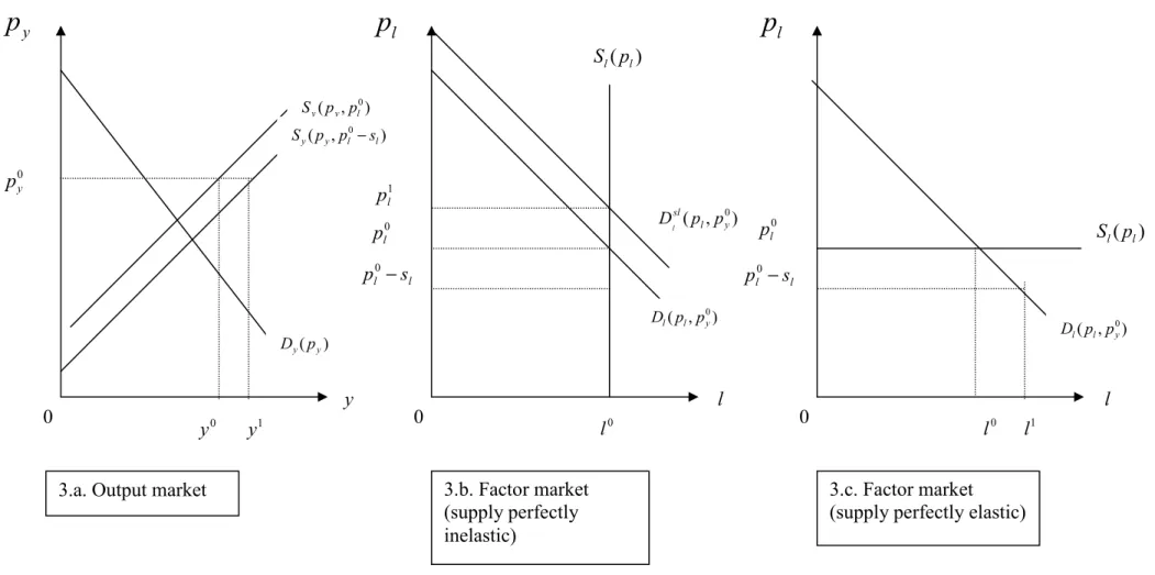
Let’s return to our previous one-factor framework. All assumptions and notations initially adopted remain, except for the policy instrument considered to support the representative farmer’s income: we assume now that this instrument is a factor subsidy (or a payment based on factor use). As depicted on figure 3, initially the farmer uses quantity l0 of the factor that he/she buys on the factor market at price p_l0 (or at opportunity cost p_l0) and produces

quantity 0

y of output that he/she sells on the output market at exogenous (world) price 0

y

p . The first incidence of the factor subsidy is to decrease the buying-in price (or the opportunity cost) of the factor for the farmer. This first incidence is represented on panels 3.b and 3.c by the decrease in the price of the factor “paid” by the farmer from p_l0 to p_l0 −s_l, where s_l is the factor subsidy.3 This reduction in the buying-in price of the factor makes the farmer’s marginal cost of output production to decrease. On panel 3.a this induced decrease in the marginal cost of production is depicted by the shift to the right of the output supply curve from S_y(p_y,p_l0) to S_y(p_y,p_l0 −s_l). Hence, at first stage, the factor subsidy generates an incentive for the farmer to increase his/her output supply: other things being equal, the farmer would seek to produce y1. However, such an output supply increase would require to use more factor. From this stage, induced adjustments on the output and factor market differ according to whether the factor supply is totally inelastic or elastic.

- In panel 3.b, as the factor supply is perfectly inelastic, the farmer cannot adjust his/her factor use up to the quantity l1 corresponding to output quantity y1. Then the factor adjustment requirement translates into a shift to the right of the factor derived demand curve from D_l(p_l,p_y0) to sl( _l, 0_y)

l p p

D . This factor demand increase translates into a

rise of both the market price (from 0

l

p to 1

l

p ) and the buying-in price (from p_l0 −s_l to

l l

l p s

p0 = 1− ) of the factor. The resulting increase in the marginal cost of y is depicted on panel 3.a through the shift back to the left of the output supply curve from

) , ( 0 l l y y p p s S − to ( , 0 1 ) l l l y y p p p s

S = − . Finally, figure 3 shows that, following the

3

The subsidy is assumed to be of the specific form, meaning that it is a total amount per unit of factor used. This kind of subsidy is similar to, and may be interpreted as, a payment based on factor use. Main results of our graphical analysis would remain valid in the case of an ad-valorem subsidy, that is a subsidy that would be defined as a percentage share of the initial equilibrium market price of the factor.

15 induced price adjustment on the factor market, the final equilibrium output quantity is unchanged at y0.

- In panel 3.c, as the factor supply is perfectly elastic, the farmer can adjust his/her factor use quantity without affecting the market price nor his/her buying-in price of

the factor (which remain at 0

l

p and p_l0 −s_l respectively). Hence, following the factor subsidy implementation, factor demand and output supply increase simultaneously, to

1

y and 1

l respectively.

Finally, figure 3 shows that the effects of the factor subsidy on both the output and factor markets are quite different according to the level of the factor supply elasticity. Figure 3 also suggests that the market effects of the factor subsidy are rather similar to those of the output

price support as described previously.4 Assuming that the considered factor is land, the lower

the land supply price elasticity the higher the share of the land subsidy “capitalised” in the rental price of land.

4

This is not so surprising in our simplified one output-one factor framework. Indeed, one guesses that, knowing the form of the production function, it may be quite easy to transform output price support into an equivalent factor subsidy and reversely. Existing theoretical literature shows however that if using more sophisticated frameworks actually makes the analysis more complex and the effects of policy instruments more ambiguous, it adds no new intuition: factor supply price elasticities do remain key parameters as regards the extent of the impact of agricultural support policy instruments on the rental price of farmland, as well as on prices of other factors and inputs, output produced and factor/input use quantities, and finally farmers income.

Figure 3. Effects of a factor subsidy on domestic output and factor markets: the one-factor case

3.a. Output market 3.c. Factor market

(supply perfectly elastic) 3.b. Factor market (supply perfectly inelastic) y

p

p

_l

p

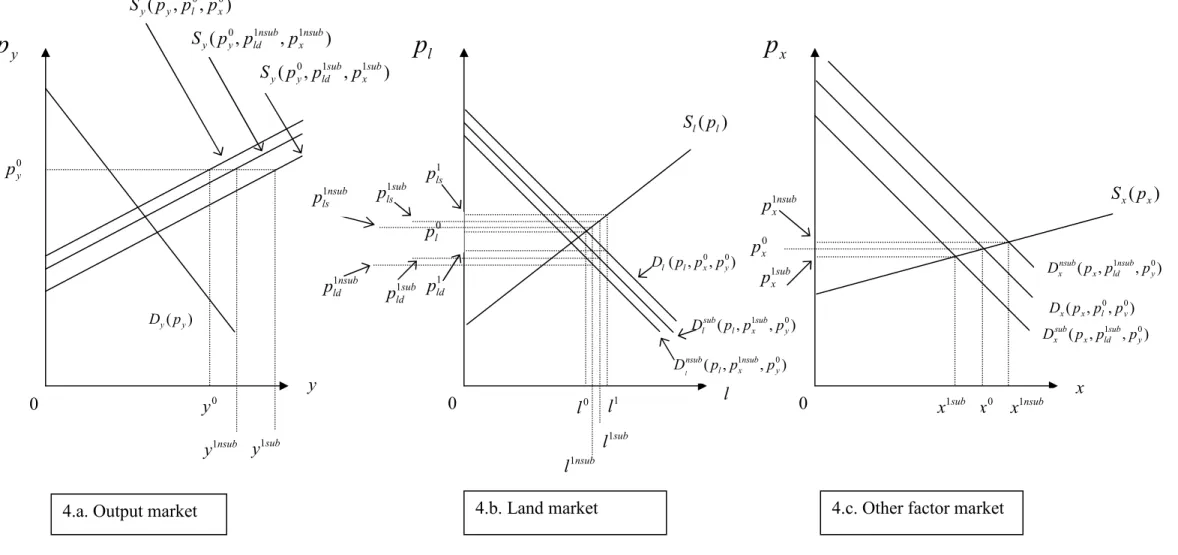
_l y l l 0 y y 0 y p 0 l p pl0 0 l l 0 1 y y l l s p0− 1 l ) , ( 0 l y y p p S ) , ( y l0 l y p p s S − ) ( y y p D ( , ) 0 y l l p p D ) , ( 0 y l l p p D ) , ( _l 0_y sl p p D l 0 0 0 ) ( _l l p S 1 l p l l s p0− ) ( _l l p S

17 The one output-two factor case: Illustrating the key role of factor substitution possibilities Let’s return to the case depicted by figure 2. We change only two assumptions. Firstly, the considered support policy instrument is no longer output price support but a land subsidy. Secondly, the supply of the other factor is now assumed to be imperfectly elastic. Therefore, the supply curve of this other factor is increasing in its price, as shown on figure 4, panel 4.c. Figure 4 indicates that at initial equilibrium, the domestic output price is 0

y

p , and the

representative farmer produces quantity 0

y , using quantity 0

l of land and quantity 0

x of the other factor. The initial rental price of land is p_l0, while the initial price of the other factor is

0 x

p .

As in the above case, described by figure 3, the first incidence of the land subsidy is to decrease the buying-in price (or the opportunity cost) of land for the farmer. This first incidence is represented on panel 4.b by the decrease in the price “paid” by the farmer from

0 l

p to p1_ld. This price decrease induces a rise in the farmer’s land demand (from l0 to l1) that, due to the relative scarcity of available land, implies an increase in the market (or supply) rental price of land up to p1_ls. As a result, the land subsidy generates a gap between the demand and the supply rental prices of land (i.e., p_ls1 −p_ld1 =s_l). Following the reduction in the buying-in price of land, the farmer’s marginal cost of production is going to decrease, inducing a shift to the right of the output supply curve. However, this shift is not represented on panel 4.a at this stage because its extent closely depends on the range of substitution possibilities between land and the other factor.

- Let’s consider first the case where land and the other factor are highly substitutable. As the land subsidy makes the buying-in price of land to decrease, the farmer has incentive to substitute land to factor x in the production process. The available technology allowing such factor substitution adjustment, the derived demand of factor

x starts to decrease (the demand curve of factor x shifts to the left on panel 4.c). However, as the supply of factor x is imperfectly elastic, the price of factor x starts to adjust down, slowing down the substitution process between land and factor x. Hence, at last a new equilibrium is reached where, as shown by panels 4.b and 4.c, both derived demand curves have shifted to the left due to factor price adjustment

interactions (from ( , 0, 0) y x l l p p p D to ( , 1 , 0) y sub x l sub l p p p

) , , ( _{x l}0 0_y x p p p D to ( , 1sub, 0_y) ld x sub x p p p

D for factor x). As both the buying-in price of

land and the price of factor x have decreased following the land subsidy

implementation, the farmer’s marginal cost of production has lowered from the initial to the final equilibrium. Hence, on panel 4.a the final output supply curve is

) , , ( 1 1sub x sub ld y y p p p

S . Therefore in this case the land subsidy induces an increase in

output quantity from 0

y to sub

y1 . This new equilibrium output quantity is obtained by

combining an increased quantity of land (from l0 to l1sub) and a decreased quantity of factor x (from x0 to _x1sub

).

- Let’s now consider the situation where land and the other factor are hardly

substitutable. In order to simplify the analysis and keep figure 4 readable, we assume that land and factor x are complementary. In such case, the first increase in land demand following the land subsidy implementation is accompanied by a simultaneous

increase in the demand of factor x (since both factors are complementary). Hence, on

factor x’s market the price starts to rise. This price increase acts as to slow down, firstly the increase in both factor demands, secondly the lowering of the farmer’s marginal production cost (following the decrease in the buying-in price of land) and finally the expansion of output supply. Hence, at last a new equilibrium is reached where on panel 4.a the final output supply curve is S_y(p_y,p_ld1nsub,p_x1nsub) and the output quantity _y1nsub

. This latter is lower than _y1sub

essentially because, contrary to the

above “substitution case”, the complementarity between land and factor x in

production prevents the farmer from exploiting fully the decrease in the buying-in

price of land by substituting cheaper land to relatively more expensive factor x. As a

result the marginal cost of production decreases less in the “complementarity case” than in the “substitution case”. For the same reason, the new equilibrium quantity use of land l1nsub is lower than the one observed in the “substitution case”, but still higher than the initial level l0 (cf. panel 4.b). However, contrary to the “substitution case”, the factor complementarity relationship makes the land subsidy induce an increase in the quantity use of factor x (from x0 to x1nsub on panel 4.c).

Finally, figure 4 shows that the effects of a land subsidy may be quite different according to the degree of factor substitution possibilities in production. First of all, figure 4 indicates that a land subsidy may induce a decrease, no change or an increase in the quantity used and the

19 market price of the non-land factors/inputs, depending on the range of substitution possibilities between land and non-land factors/inputs, from strong substitutes to complements. Secondly, figure 4 shows that, while the land subsidy unambiguously induces an increase in the output supply quantity, the extent of this increase closely depends on the degree of land and non-land factor/input substitution in production: the higher the substitution possibilities, the greater the output supply increase. Thirdly, figure 4 indicates that, while the land subsidy unambiguously induces an increase in the rental market price of land, a decrease in the corresponding buying-in price for the farmer and an increase in the land use quantity, the extent of these adjustments closely depends on the land to non-land factor/input substitution possibilities: the higher the substitution possibilities, the greater the increase in both the land use quantity and the rental market price of land.

It is interesting to point out at this stage that the overall support provided through the land subsidy is shared between the farmer, the landowner and the non-land factor/input supplier. Whatever the factor substitution possibilities, both the farmer and the landowner experience a gain resulting from, respectively, the decrease in the buying-in price of land and the increase of its market price. The gain for both agents is however greater when land and non-land factors/inputs are strong substitutes in production, since in that case the benefit of support is not shared with the non-land factor/input supplier. Indeed in that case the non-land factor/input supplier may experience a loss, part of his/her surplus being transferred to the farmer via the decrease in the non-land factor/input price and to the landowner via the stronger increase in derived demand on the land rental market. At reverse and as shown by figure 4, when land and non-land factors/inputs are complements in production, the non-land factor/input supplier may experience a gain that reduces the benefit for the farmer and the landowner.

Figure 4. Effects of a land subsidy on domestic output and factor markets: the two-factor case

4.a. Output market 4.b. Land market 4.c. Other factor market

y

p

p

_l

p

_x y l x 0 y y 0 y p 0 l p 0 x p 0 l l1 x0 y 1 ld p sub x1 ) ( y y p D ( , , ) 0 0 y l x x p p p D ) , , ( 1 0 y nsub x l nsub p p p D l ) , , ( 1 0 y sub x l sub l p p p D ) , , ( 1 0 y sub ld x sub x p p p D 0 0 0 sub y1 nsub y1 ) , , ( 0 0 y x l l p p p D 1 ls p ) , , ( 1 0y nsub ld x nsub x p p p D sub l1 ) ( _l l p S ) ( _x x p S nsub x1 sub ls p1 nsub ls p1 nsub l1 sub ld p1 nsub ld p1 nsub x p1 sub x p1 ) , , ( 0 1 1sub x sub ld y y p p p S ) , , ( 0 1 1nsub x nsub ld y y p p p S ) , , ( _{y l}0 0_x y p p p S

21 Finally, as regards the impact of the land subsidy on land rental market and price, one may synthesise the main findings as follows.

For given supply price elasticities of land and non-land factors/inputs, the higher the substitution elasticity between land and non-land factors/inputs:

- The higher the increase in the rental market price of land and, thus, the higher the amount of support “capitalised” in the rental price of land.

- The greater the decrease in the production cost of the output (and the higher the positive effect of the land subsidy on output supply quantity).

- The higher the gain for the farmer in terms of increased surplus and the higher the amount of support transferred to the landowner.

Comparing the effects of both the output price support and the land subsidy instruments one may draw the main following insights (still for given supply price elasticities of land and non-land factors/inputs):

- Both instruments are expected to increase output supply, and for both instruments the

higher the degree of substitution between land and non-land factors/inputs, the greater the extent of the output increase.

- Both instruments are expected to increase land use and land rental price. For the output price support instrument, the higher the degree of substitution between land and non-land factors/inputs, the lower the extent of land use and land rental price increases. At reverse, for the land subsidy instrument, the higher the degree of substitution the greater the extent of land use and land rental price increases. The main reason for this reverse impact of the substitution possibilities lies in the differentiated first incidences of both instruments. The first incidence of the output price support instrument is to generate an incentive for the farmer to increase output supply. As expanding output requires using more factors/inputs, this first incidence then spreads within all factor and input markets. And the higher the substitution possibilities between factors/inputs, the greater the dilution of support across factors/inputs. In other words the higher the substitution possibilities, the less the support is allowed to concentrate on one specific factor or input (in our example, land). At reverse, the first incidence of the land subsidy is to decrease the buying-in price of land for the farmer. Hence, in this case the support initially concentrates on land and then spreads within the output and other factor/input markets. But the higher the substitution possibilities

between land and non-land factors/inputs, the more the farmer can increase his/her land use and consequently the less the support is allowed to spread within non-land markets.

The previous graphical analysis does not allow to conclude about the comparative effect on output supply of the same amount of support given through either the output price support or the land subsidy instrument. However, Hertel (1989), Dewbre et al. (2001) and Guyomard et al. (2004), using different frameworks (and hence different assumptions), have obtained some analytical results to this regards.

- Under constant return to scale assumption, perfectly elastic supplies of non-land inputs

and imperfectly elastic land supply, Hertel (1989) shows that an input subsidy will have greater impact on output supply than an equal cost output subsidy, provided the subsidised input substitutes for land. Contrary to our case, the subsidised input in Hertel’s study is not land but a non-land input with a perfectly elastic supply. And this is exactly because the subsidy is applied to an input with perfectly elastic supply, that Hertel obtains the above presented result.

- In Dewbre et al. (2001) the subsidy is alternatively applied to land and non-land inputs

and the supply of both categories of inputs may be perfectly/imperfectly elastic or perfectly inelastic. Under assumptions of constant return to scale and small country, Dewbre et al. show that market price support will have greater impact on output supply than an equal cost land subsidy (or payment based on area) if the elasticity of supply of land is lower than that of the non-land inputs.

- In a more general framework (no constant return to scale assumption, no small country

assumption, free entry and exit in the agricultural sector) Guyomard et al. (2004) show that an output subsidy will unambiguously have greater impact on output supply than an equal cost land subsidy. The authors also demonstrate that an output subsidy will unambiguously have lower impact on land rental price than an equal cost land subsidy. In other words, and conform to the intuition that arises from our previous graphical analysis, a larger part of support is “capitalised” in the rental price of land when this support is provided through a land subsidy than through output price support.

At this stage, it is interesting to point out that the current evolution of agricultural policies in most industrialised countries is likely to reinforce the capitalisation of support in the farmland rental price. Indeed, according to Guyomard et al.’s result, the decapitalisation of support that

23 should follow the decrease in the support based on output should be more than counterbalanced by the intensification of capitalisation of support that should follow the increase in support based on area. Of course, there are a lot of other factors that can influence the evolution of farmland rental prices in industrialised countries (such as legal factors for instance, see e.g., OECD, 1996; Latruffe and Le Mouël, 2006). In addition, the land subsidy as designed in Guyomard et al. (2004) and in this paper does not fit the much more complex area payment systems that some countries have actually implemented. However, this is a matter of fact that the current evolution of agricultural policies in industrialised countries mainly consists in replacing market price support instruments through which the support is based on output and likely to “capitalise” less in farmland rental prices, by direct payment systems through which the support is most often (explicitly or implicitly) based on area and likely to “capitalise” more in farmland rental prices.

3. Empirical review

3.1. A methodological note

Empirical estimations of farmland price formation

In the mid-60’s the common approach to farmland pricing was to use a supply-demand framework with the quantity of land supplied for sale as an ad-hoc function of the price of land and other variables (urban pressure for example) and the demand for land as an ad-hoc function of the price of land and other variables (such as net farm income or productivity increase for example) (e.g. Herdt and Cochrane, 1966; Tweeten and Martin, 1966; Reynolds and Timmons, 1969; Cowling et al., 1970). Harvey (1974) pointed out however that such an approach is theoretically incorrect for two reasons. Firstly, there is not a stable relationship between the number of transactions and the supply of or demand for land. Given that transactions merely restore equilibrium, a given price may be associated with a large number of transactions or no transactions. Secondly, the same factors (farm incomes, riskiness, capital gains prospects, etc.) cause shifts in both the supply and the demand functions. Therefore, their separate influences cannot be identified. Due to these theoretical and other empirical unresolved problems, following studies focused exclusively on the role of demand side forces. For this, most studies have relied on the present value model (PVM). This model stipulates that the price of an income-earning asset is equal to the discounted expected value of the stream of future net returns or rents to this asset. Hence, according to the PVM, the price of farmland should be driven essentially by the discounted expected value of the stream of future

net returns to farming or rents. Assuming that the value of an income-producing asset is the capitalised value of the current and future stream of earnings from owning this asset, the equilibrium asset price at the beginning of time period t (Lt) may be written as:

( )

(

)(

) (

)

∑

∞ = + + + + + + + = 0 1 1 1 2 ...1 i t t t i i t t r r r R E L (1)

where Rt is the net real return at the end of time period t, generated from owning the asset, rt

is the time varying real discount rate for year t and E is the expectation on return conditional on information in period t.

If it is assumed that the net return is constant in each period (R*), that the discount rate is constant, that agents are risk neutral and that differential tax treatments of capital gains and rental income are ignored, then equation [1] simplifies to the basic capitalisation formula:

r R Lt

*

= (2)

This basic capitalisation formula underlies most of the studies concerned with farmland price formation, with Lt as farmland value or price and Rt as the real net return to farmland (most

often measured by net farm income or some -cash- rent). However, equation [2] is derived under very restrictive assumptions and actually most of existing studies used refined versions of the basic capitalisation formula, that were obtained in much more flexible frameworks. Major modifications of the basic capitalisation formula were: introducing the growth in earnings from land (Melichar, 1979; Baker et al., 1991), allowing for differential tax treatment of income and capital gains (Alston, 1986; Burt, 1986), and considering the role of inflation (Feldstein, 1980). Other refinements comprised accounting for credit market imperfections (Shalit and Schmitz, 1982), modifying the expectation schemes (Lloyd et al., 1991; Just and Miranowski, 1993), incorporating risk and risk aversion (Chavas and Jones, 1993), including transaction costs (Shiha and Chavas, 1995), and taking into account potential returns from non-agricultural uses (Robison et al., 1985; Plantiga and Miller, 2001; Plantiga et al., 2002).

A number of studies using co-integration techniques questioned the empirical finding, based on the PVM, that net real returns are the major factor explaining land values (Campbell and Shiller, 1987; Falk, 1991; Hallam et al., 1992; Clark et al., 1993). If the PVM is correct, then land rents and land prices should have the same time series properties, and the spread, defined as the stationary linear relationship between land rents and prices, should add useful

25 information in forecasting future changes in rents given past changes in rents. A number of studies tested for two main reasons of rejection of the PVM: time-varying discount rates (Falk, 1992; Hanson and Myers, 1995) and the presence of speculative bubbles (Featherstone and Baker, 1988; Tegene and Kuchler, 1993; Falk and Lee, 1998). Following this literature, co-integration testing has become a routine in many studies, as a preliminary step before the empirical application of the PVM.

Empirical investigation of the capitalisation of public support

Capitalisation of public support in farmland prices has been mostly investigated with the help of the PVM, by separating the return to land (R) into two sources of income: a market-based source and a government-based source. This method has been applied as such (Goodwin and Ortalo-Magné, 1992; Clark et al., 1993; Clark et al., 1993) or by specifying different discount rates (r) for the two sources of income (Weersink et al., 1999; Duvivier et al., 2005). Two studies have accounted for the counter-cyclical nature of government payments, that is to say the inverse relationship between these payments and the land returns, by adding an equation explaining the amount of the payments as a function of several determinants including the returns to land (Shaik et al., 2005; Shaik et al., 2006). In many studies the basic PVM has been modified in the same lines as explained above: assuming time-varying rates (Vantreese et al., 1989; Cavailhès and Degoud, 1995; Weersink et al., 1999; Flanders et al., 2004), treating expectations with various schemes (Cavailhès and Degoud, 1995; Duvivier et al., 2005; Goodwin et al., 2005), accounting for alternative land uses (Goodwin et al., 2003 and 2005). Several studies have also econometrically tested the appropriateness of the PVM (Weersink et al., 1999; Flanders et al., 2004, Duvivier et al., 2005).

The investigation of the issue has, however, not always relied on the PVM approach. A few studies based their investigation on the hedonic pricing approach (Barnard et al., 1997; ERS USDA, 2001b; Taylor and Brester, 2005). This approach, standard in consumer research and environmental valuation, was firstly applied to land by Palmquist (1989). The interpretation of the hedonic function is that observed prices of a product are explained by a vector of specific amounts of quality components. In practice however, the components entering the hedonic function are usually chosen without theoretical justification; government payments are thus among these components. Finally, the investigation of the effect of agricultural policy on land rents has often been carried out using the agricultural producer’s framework, that is to say maximising farmers’ profit, that includes rentals (Lence and Mishra, 2003; Roberts et al., 2003).

3.2. Empirical results from the literature

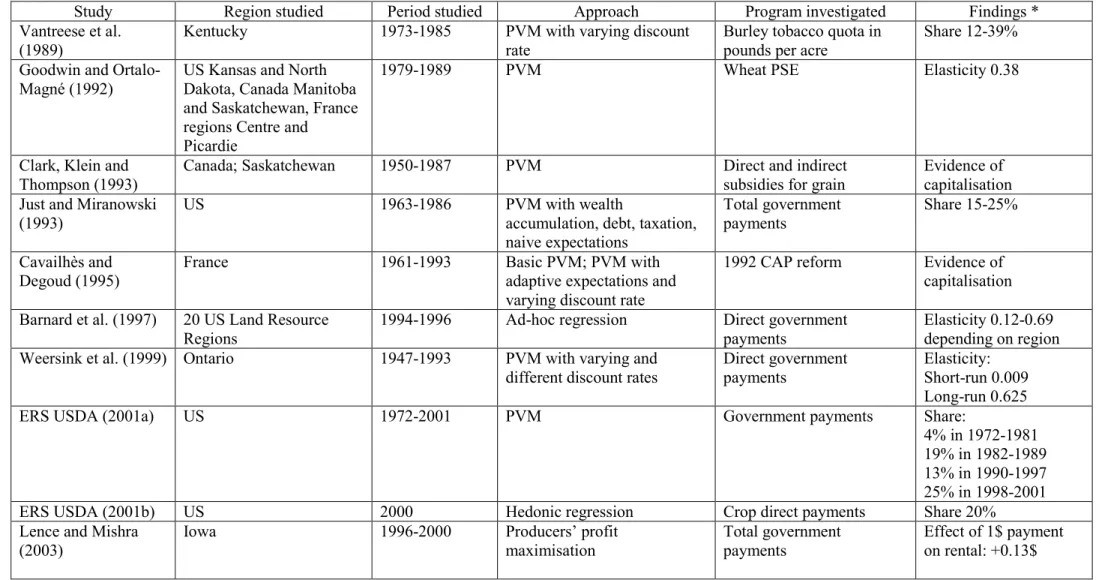
While some studies have simply given evidence of the capitalisation of public support without quantifying it (Clark et al., 1993; Cavailhès and Degoud, 1995; Flanders et al., 2004), this article focuses on the quantitative results from the studies, that is to say the extent of capitalisation. This is assessed in terms of the responsiveness of the land values with respect to the support, and of the share of land value that can be attributed to Farm programs. Farm programs cover both income support (through market price support, output or factor/input subsidies or direct government payments for instance) and output supply or input use control (production quota or acreage restrictions for example). Most studies existing in the literature investigated the capitalisation of direct government payments, whether total or several types of payments. All findings are summarised in table 1.

Responsiveness of the land values with respect to the support

Only one study reported the effect of one additional dollar of payment on land prices: Goodwin et al. (2005) found that usually one dollar of government payment resulted in an increase of 13.44 dollars of land price in the US. Studies about the effect of one additional dollar of payment on land rents found an increase of less than one dollar of rental (Lence and Mishra, 2003; Roberts et al., 2003; Goodwin et al., 2005) in the US in the second half of the 90es (except for Roberts et al., 2003). As indicated by some authors, this dilution can be explained by the fact that, in the case of some support programs, farmers have to fulfil some requirements such as set-asides which imply reduced income. Cross-compliance requirements might also decrease farm income by imposing maintenance costs. Rutherford et al. (1990) also gave evidence of this dilution effect using a General Equilibrium model of global trade in wheat calibrated with 1981 data. The authors forecasted that the capitalisation rate of the US wheat price support program was 25%, meaning that 75% of the capitalisation was diluted. They explained this result by the conditionality of the support: set-aside requirements imply additional costs for participants, which might offset the benefit of the support.

One must underline here that, at least for farmland rental prices, theoretical insights presented in the previous section clearly show that, even in the absence of set-aside or cross-compliance requirements, such dilution of support commonly arises since only very specific assumptions on the land supply price elasticity, on the relative levels of factors and inputs supply price elasticities and on factors/inputs substitution possibilities are required for one dollar of support is totally “capitalised” in farmland rental price.

27 Numerous studies report elasticity estimates of land prices with respect to public farm programs. And all of them found an estimate less than one (Goodwin and Ortalo-Magné, 1992; Barnard et al., 1997; Wersink et al., 1999; Duvivier et al., 2005; Taylor and Brester, 2005; Shaik et al., 2005; Latruffe et al., 2006; Shaik et al., 2006), whether the analysis was for the US, Canada, France, Belgium or the Czech Republic, in the 80es, 90es, or second half of the century. This inelastic response could be explained by the way agents discount the government payments. Were the latter seen as transitory, they would be heavily discounted, implying a lower elasticity of response. The agents would however discount less heavily payments that they would consider permanently available. In other words, if agents have doubts about the certainty of farm programs, land prices will be lower than if payments were to continue indefinitely. Schmitz (1995) was the first one to highlight this uncertainty issue, by showing that Ricardian rents (including government payments) and wealth did not bear a one-to-one relationship for the Canadian Prairie region in 1982-1986. By contrast, Weersink et al. (1999) found that in Ontario during 1947-1993 government payments were less heavily discounted than market returns: the former were thus considered as more stable by farmers. Studies usually concord regarding the comparison of responsiveness with respect to government payments and to market-based returns. Most of the analyses having investigated this issue show that land prices are more responsive to the former than to the latter (Goodwin et al., 2005; Duvivier et al., 2005; Taylor and Brester, 2005; Latruffe et al., 2006; Shaik et al., 2006). Two studies found the opposite (Goodwin and Ortalo-Magné, 1992; Shaik et al., 2005), but Weersink et al. (1999) showed that it was actually in the long run that land prices were more responsive to government payments than to market-based returns, while the reciprocal was true in the short run.

Share of land value that can be attributed to the support

Only studies in the US have investigated the share of land price that can be attributed to public programs (Vantreese et al., 1989; Just and Miranowski, 1993; ERS USDA, 2001a and 2001b; Shaik et al., 2005; Shaik et al., 2006). Despite the difference in the type of program (all government payments, crop direct payments only, burley tobacco quotas), studies consistently report that a substantial share of land prices is due to government payments: in general between 12% and 40%, with peaks at 4% (total government payments in 1970-1979; ERS USDA, 2001a) and 67% (total government payments in the US Southern states during the last Farm Bill; Shaik et al., 2006).

Table 1: Summary of the studies having investigated empirically the extent of capitalisation

Study Region studied Period studied Approach Program investigated Findings * Vantreese et al.

(1989)

Kentucky 1973-1985 PVM with varying discount rate

Burley tobacco quota in pounds per acre

Share 12-39% Goodwin and

Ortalo-Magné (1992)

US Kansas and North Dakota, Canada Manitoba and Saskatchewan, France regions Centre and Picardie

1979-1989 PVM Wheat PSE Elasticity 0.38

Clark, Klein and Thompson (1993)

Canada; Saskatchewan 1950-1987 PVM Direct and indirect subsidies for grain

Evidence of capitalisation Just and Miranowski

(1993)

US 1963-1986 PVM with wealth

accumulation, debt, taxation, naive expectations Total government payments Share 15-25% Cavailhès and Degoud (1995)

France 1961-1993 Basic PVM; PVM with adaptive expectations and varying discount rate

1992 CAP reform Evidence of capitalisation Barnard et al. (1997) 20 US Land Resource

Regions

1994-1996 Ad-hoc regression Direct government payments

Elasticity 0.12-0.69 depending on region Weersink et al. (1999) Ontario 1947-1993 PVM with varying and

different discount rates

Direct government payments

Elasticity: Short-run 0.009 Long-run 0.625 ERS USDA (2001a) US 1972-2001 PVM Government payments Share:

4% in 1972-1981 19% in 1982-1989 13% in 1990-1997 25% in 1998-2001 ERS USDA (2001b) US 2000 Hedonic regression Crop direct payments Share 20%

Lence and Mishra (2003)

Iowa 1996-2000 Producers’ profit maximisation

Total government payments

Effect of 1$ payment on rental: +0.13$

29

Roberts et al. (2003) US 1992 and 1997 Producers’ profit maximisation PFC payments without conservation payments Effect of 1$ payment on rental: +0.23-0.76$ in 1992, +0.33-1.55$ in 1997 Flanders et al. (2004) Georgia 1967-2002 PVM Total government

payments Evidence of capitalisation Goodwin et al. (2005) (improvement of Goodwin et al., 2003) US 1998-2001 PVM with non-agricultural uses; account for expectations by averaging past values

Total government payments Effect of 1$ payment on land price: +13$ Effect of 1$ payment on cash rent: +0.35$ Effect of 1$ payment on share rent: +0.51$ Duvivier et al. (2005) Belgium 1980-2001 PVM with different discount

rates; account for

expectations by averaging past values

Crop direct payments Elasticity 0.17-0.34 depending on year

Shaik et al. (2005) US 1940-2002 PVM accounting for counter-cyclicality of payments

Total government payments

Elasticity 0.35 Share 30% Taylor and Brester

(2005)

Montana 1986-1999 Hedonic regression Domestic price of sugar beet (kept high due to import restrictions)

Elasticity 0.16

Latruffe et al. (2006) Czech Republic 1995-2001 PVM with non-agricultural uses

Direct payments Elasticity 0.13 Shaik et al. (2006) US; Southern vs. other

states

1940-2004 PVM accounting for counter-cyclicality of payments Total government payments Elasticity 0.12 in 2002-2004 Share up to 65% in Southern states PVM: Present value model. PSE: production support estimate. CAP: Common Agricultural Policy. PFC: production flexibility contracts.

4. Conclusion

This article has shown that agricultural production theory allows to derive some general insights as regards the impact of various policy instruments on the rental price of farmland. These main insights may be summarised as follows:

- agricultural support policy instruments contribute to increase the rental price of farmland;

- the extent of this increase closely depends on the level of the supply price elasticity of

farmland relative to those of other factors/inputs on the one hand, the range of the possibilities of factor/input substitution in agricultural production on the other hand;

- whatever the policy instrument, the lower the elasticity of farmland supply, the higher

the increase in the rental price of farmland;

- for the output price support instrument, the higher the degree of substitution between

land and non-land factors/inputs, the lower the extent of land use and land rental price increases. At reverse, for the land subsidy instrument, the higher the degree of substitution, the greater the extent of land use and land rental price increases;

- as shown by some authors, an output subsidy will unambiguously have lower impact

on land rental price than an equal cost land subsidy. In other words, a larger part of support is “capitalised” in the rental price of land when this support is provided through a land subsidy than through output price support.

The impact of agricultural policies on the selling price of farmland has very rarely been examined from a theoretical point of view. Indeed it is commonly assumed in existing studies that the buying and selling prices of farmland can be adequately approximated by the discounted sum of future rental prices, so that a prediction about the direction of the rental prices is equivalent to a prediction about the direction of the buying and selling prices. As a result, most theoretical work has focused on the rental price of farmland.

The review of empirical literature regarding the impact of agricultural policy on farmland values identified several relevant papers written from the late 80es. Despite the wide differences between the studies in terms of method and data, one can try to summarise the findings in a few main points.

- Government payments and other types of support (price support, quotas) are

31 but they also account for a large share of the land prices. In general studies agree about a share around 15-30%, although it could be up to 70% depending on specific regions and dates.

- Land prices and rents have a significant positive response to government support.

Although the magnitude of the response varies across studies5, it has almost consistently been showed to be less than 1. Such inelastic response is thought to reflect the uncertain future of the farm programs. However, there is no consensus about whether government payments are discounted more heavily (that is to say, are seen as more transitory) than market earnings. Despite this, in general studies have indicated that land prices are more responsive to government-based returns than to market-based returns.

Although some contradictions remain among findings from the empirical studies, what appears clearly is that part of the payments are capitalised in land prices, implying that governments could have partially missed their target of providing income support to farmers. It is also clear that the way agents see the policy (credible, transitory) has crucial implications for the welfare of farmers.

5

Oltmer and Florax (2001) attempted to compare statistically the findings from 17 different studies reporting elasticities of land prices with respect to earnings including farm support. Using meta-analysis based on several factors regarding the methodology, the commodity supported, the location, the period and the type of data, they found no significant differences between elasticities of land prices with respect to land returns according to the methodology used. They also reported that the elasticities with respect to returns in which both price support and income support were included, were higher than with respect to returns including only one type of support.

References

Alston, J.M. (1986). An analysis of growth of US farmland prices, 1963-82. American Journal of Agricultural Economics, 68(1): 1-9.

Baker, T.G., Ketchabaw, E.H., Turvey, C.G. (1991). An income capitalization model for land value with provisions for ordinary income and long-term capital gains taxation. Canadian Journal of Agricultural Economics, 39(1): 69-82.

Barnard, C.H., Whittaker, G., Westenbarger, D., Ahearn, M. (1997). Evidence of capitalization of direct government payments into U.S. cropland values. American Journal of Agricultural Economics, 79(5): 1642-1650.

Burt, O.R. (1986). Econometric modeling of the capitalization formula for farmland prices. American Journal of Agricultural Economics, 68(1): 10-26.

Campbell, J.Y., Shiller, R.J. (1987). Cointegration and tests of present value models. Journal of Political Economy, 95(4): 1062-1088.

Cavailhès, J., Degoud, S. (1995). L’évaluation du prix des terres en France: Une application de la réforme de la PAC. Cahiers d’Economie et Sociologie Rurales, 36: 49-77.

Chavas, J.P., Jones, B. (1993). An analysis of land prices under risk. Review of Agricultural Economics, 15: 351-366.

Clark, J.S., Fulton, M., Scott, J.T.Jr. (1993). The inconsistency of land values, land rents, and capitalization formulas. American Journal of Agricultural Economics, 75: 147-155.

Clark, J.S., Klein, K.K., Thompson, S.J. (1993). Are subsidies capitalized into land values? Some time series evidence from Saskatchewan. Canadian Journal of Agricultural Economics, 41: 155-168.

Cowling, K., Metcalf, D., Rayner, A.J. 1970. Resource structure of agriculture: An economic analysis. Pergamon Press, Oxford.

Dewbre, J., Anton, J., Thompson, W. (2001). The transfer efficiency and trade effects of direct payments. American Journal of Agricultural Economics, 83(5): 1204-1214.

Dewbre, J., Short, C. (2002). Alternative policy instruments for agriculture support: Consequences for trade, farm income and competitiveness. Canadian Journal of Agricultural Economics, 50(4): 443-464.

33 Duvivier, R., Gaspart, F., Henry de Frahan, B. (2005). A Panel Data analysis of the Determinants of Farmland Price: An Application to the Effects of the 1992 CAP Reform in Belgium. Paper presented at the XIth European Association of Agricultural Economists Congress, Copenhagen, Denmark, 23-27 August.

ERS USDA. (2001a). Government Payments to Farmers Contribute to Rising Land Values. Agricultural Outlook June-July 2001. Economic Research Service, United States Department of Agriculture, Washington DC.

ERS USDA. (2001b). Higher Cropland Value from Farm Program Payments: Who Gains? Agricultural Outlook November 2001. Economic Research Service, United States Department of Agriculture, Washington DC.

Falk, B. (1991). Formally testing the present value model of farmland prices. American Journal of Agricultural Economics, 73(1): 1-10.

Falk, B. (1992). Predictable excess returns in real estate markets: A study of Iowa farmland values. Journal of Housing Economics, 2: 84-105.

Falk, B., Lee, B.S. (1998). Fads versus fundamentals in farmland prices. American Journal of Agricultural Economics, 80: 696-707.

Featherstone, A.M., Baker, T.G. (1988). Effects of reduced price and income supports on farmland rent and value. North Central Journal of Agricultural Economics, 10(1): 177-90. Feldstein, M. (1980). Inflation, portfolio choice and the prices of land and corporate stocks.

American Journal of Agricultural Economics, 62(4): 532-546.

Flanders, A., White, F.C., Escalante, C.L. (2004). Comparing Land Values and Capitalization of Cash Rents for Cropland and Pasture in Georgia. Paper presented at the Southern Agricultural Economics Association Annual Meeting, Tulsa, Oklahoma, 14-18 February. Floyd, J.E. (1965). The effects of farm price supports on the returns to land and labor in

agriculture. Journal of Political Economy, 73: 148-158.

Gardner, B.L. (1987). The Economics of Agricultural Policies. New-York, Macmillan.

Gisser, M. (1993). Price support, acreage controls, and efficient redistribution. Journal of Political Economy, 101(4): 584-609.

Goodwin, B.K., Ortalo-Magné, F. (1992). The capitalization of wheat subsidies into agricultural land values. Canadian Journal of Agricultural Economics, 40(1): 37-54.