HAL Id: cea-02927382
https://hal-cea.archives-ouvertes.fr/cea-02927382
Submitted on 1 Sep 2020
HAL is a multi-disciplinary open access
archive for the deposit and dissemination of
sci-entific research documents, whether they are
pub-lished or not. The documents may come from
teaching and research institutions in France or
abroad, or from public or private research centers.
L’archive ouverte pluridisciplinaire HAL, est
destinée au dépôt et à la diffusion de documents
scientifiques de niveau recherche, publiés ou non,
émanant des établissements d’enseignement et de
recherche français ou étrangers, des laboratoires
publics ou privés.
Precise determination of the conductivity exponent of
3d percolation using ”Percola”
Jean-Marie Normand, Hans J. Herrmann
To cite this version:
Jean-Marie Normand, Hans J. Herrmann. Precise determination of the conductivity exponent of 3d
percolation using ”Percola”. 1996. �cea-02927382�
arXiv:cond-mat/9602081v1 14 Feb 1996
International Journal of Modern Physics C c
World Scientific Publishing Company
PRECISE DETERMINATION OF THE CONDUCTIVITY EXPONENT OF 3D PERCOLATION USING “PERCOLA”
JEAN-MARIE NORMAND1and HANS J. HERRMANN2
1 CEA, Service de Physique Th´eorique, CE-Saclay
F-91191 Gif-sur-Yvette Cedex, FRANCE
2 P.M.M.H., E.S.P.C.I., 10 rue Vauquelin
75231 Paris Cedex 05, France
Using 20 months of CPU time on our special purpose computer “Percola” we determined the exponent for the normal conductivity at the threshold of three-dimensional site and bond percolation. The extrapolation analysis taking into ac-count the first correction to scaling gives a value of t/ν = 2.26±0.04 and a correction exponent ω around 1.4.
1. Introduction
Percolation [1] is the simplest model for a random medium and is applied to
describe porous media, gelation, mixtures of electrical conductors, and many other disorder dominated situations. It is defined on a lattice by occupying with probabil-ity p randomly and independently either the sites or the bonds with conductors. If one considers that locally current can only flow between conductors that are nearest neighbors, then only above a critical value pc a global current can flow through the
system. The global electrical conductivity Σ rises like
Σ ∼ (p − pc)t (1)
and the accurate determination of t, or more precisely of t/ν where ν is the exponent of the correlation length, is the aim of the present paper.
In the ’80s, after a heated controversy the critical exponents for the conductivity of two-dimensional percolation were determined quite accurately [2,3] and various
conjectures [4] could be ruled out. The three-dimensional situation remained less
clear because of the larger error bars. Only recently new efforts have been made[5,6]
computational means. Gingold and Lobb[5]find t/ν = 2.276 ± 0.012 and Batrouni
et al.[6] claim t/ν = 2.282 ± 0.005.
Using the specially constructed processor “Percola”[7], assembled in Saclay by
J.-M. Normand and M. Hajjar between 1984 and 1987, we did exact calculations on narrow bars of random conductors (“strip-bar method”), a technique that has given very precise values in two dimensions [2] and for the superconducting-conducting
mixture in three dimensions [8]. For the three-dimensional conductivity problem
treated in this paper this method a dozen years ago gave t/ν = 2.2 ± 0.1, however, with much smaller computational investment[9].
In the following section we describe the methods, in the next section we present our results and analyze them, and finally we conclude.
2. Method
The method we use[9]is a straightforward generalization to three dimensions of
the technique of Derrida and Vannimenus [10]. We calculate the electrical current
on a simple cubic lattice of width m and depth n in the horizontal directions, and of length L vertically, growing from bottom up. Periodic boundary conditions are used in the y-direction, defined in fig. 1. Each bond between nearest neighbors is randomly conducting, in bond percolation if the bond is occupied (with probability p), in site percolation if both neighbors are occupied (each with probability p), otherwise it is insulating. The top and the bottom planes are two equipotentials (fixed boundary condition). One defines by Ii and Vi the current and potential
at the end of each line i, i = 1 being the index associated with the top plane. The conductance matrix σi,j, given through Ii = Pn·m+1i=1 σi,jVj, is updated via
σ′
i,j = σi,j−σi,ασα,jr/(1 + σα,αr) if a longitudinal bond is added at line α and
via σ′
i,j= σi,j+ (δα,j−δβ,j) · (δα,i−δβ,i)/r if a transversal bond is added between
lines α and β where r is the resistance of the bond. In that way the conductance is obtained exactly. A very large L (bar configuration) automatically averages over many configurations leaving no ambiguity over whether one should average the conductivity, the resistivity, or functions of them. This is an advantage over methods that average over many disjoint cubes[3,5,6,10].
Fig. 1 Bar of lengthL, widthmand depthn. We calculate the conductivity between the two black planes.
We will consider, as in[9], the cases m = n−1 for bond percolation and m = n for
site percolation. The conductance of the bar per length is then σ1,1/L which in the
limit L → ∞ goes to a value σn. The calculation is performed for different linear
sizes n at the percolation threshold pc = 0.248812 [11] for bond percolation and
pc= 0.311605[11] for site percolation. The critical exponent t/ν is then extracted
by using the finite size scaling:
σn= an−t/ν(1 + bn−ω) (2)
where a and b are non-universal constants and ω is the (first) universal correction to scaling exponent. Since ν, the correlation length exponent, is known rather precisely (ν = 0.875 ± 0.003)[11] one can determine t.
3. Results and Analysis
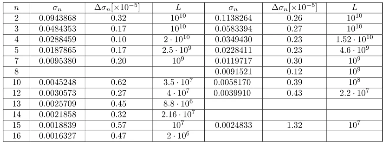
The values obtained with “Percola” using a CPU time of 20 months are given in table 1 for the case of bond and of site percolation. Percola[7], a 64-bit floating point
processor runs at 25 MFlops but is specialized to deal with the algorithm described in the previous section for which it runs faster than a Cray-XMP mono-processor. The lengths of the bars presented in table 1 exceed those calculated before [9] by
about a factor of 1000. n σn ∆σn[×10−5] L σn ∆σn[×10−5] L 2 0.0943868 0.32 1010 0.1138264 0.26 1010 3 0.0484353 0.17 1010 0.0583394 0.27 1010 4 0.0288459 0.10 2 · 1010 0.0349430 0.23 1.52 · 1010 5 0.0187865 0.17 2.5 · 109 0.0228411 0.23 4.6 · 109 7 0.0095380 0.20 109 0.0119717 0.30 109 8 0.0091521 0.12 109 10 0.0045248 0.62 3.5 · 107 0.0058170 0.39 108 12 0.0030573 0.27 4 · 107 0.0039910 0.43 2.2 · 107 13 0.0025709 0.45 8.8 · 106 14 0.0021858 0.32 2.16 · 107 15 0.0018839 0.57 107 0.0024833 1.32 107 16 0.0016327 0.47 2 · 106
Table 1 Conductance σn per length for bond (left) and site (right) percolation for
different widths n of the bar. We also show the statistical mean square deviation
∆σn and the lengthLof the bar for each case.
We analyzed the data with various techniques. Finding that t/ν which minimizes the squared error for fixed ω (as done in refs. [2] and [8]) gives t/ν = 2.15 ± 0.12 for the sites and t/ν = 2.26 ± 0.06 for the bonds. In both cases ω ≈ 1.4 gave the best fits. Since universality states that these exponents should be the same only the intersection of the error bars, i.e. t/ν = 2.23 ± 0.06, should be relevant.
The data for bond percolation are closer to the asymptotic regime as can be seen from the error bars and the curvature in a plot log(σnnt/ν) against n−ω. Looking for
bond percolation at successive slopes (local derivative of log(σ) vs log(n)) against n−ωgives the most plausible curve for ω around 1.4. In that case t/ν = 2.25 ± 0.05.
Keeping t/ν fixed and finding the ω which minimizes the error (and number of iterations) in the Runge-Kutta procedure of minimizing the mean square deviation, gives a dependence t/ν against ω as shown in fig. 2. For ω around 1.4 we find t/ν = 2.26 ± 0.04 for bond percolation. Unfortunately, as opposed to the case of the superconductivity exponent[8]the prefactor of the site percolation data has the
same sign as for bond percolation. Therefore the curves for site percolation in fig. 2 do not intersect with those of bond percolation which does not allow us to increase the precision by assuming universality and combining the two data sets.
Fig. 2 Leading exponentt/ν against the first correction exponentωfor bond perco-lation omitting all sizes of width less or equal tonl, fornl= 2(diamonds), 3 (crosses
+), 4 (squares) and 5 (crosses x).
4. Conclusion
Although we have obtained extremely precise data for the conductance of nar-row systems our error bars for the exponents t/ν extrapolated to infinite sizes are not as small as obtained by other methods [5,6]. This is due to the fact that we
have seriously taken into account the first corrections to scaling which seems im-perative for the case of small systems. As with many simulations of high precision,
statistical errors are much smaller than the systematic ones. In contrast to the two-dimensional case [2] and the superconducting case in three dimensions [8] the
relation between leading and correction exponent is not in opposite sense for site percolation as compared to bond percolation giving us a particularly unlucky sit-uation. We conclude t/ν = 2.26 ± 0.04 consistent with previous values and the Alexander-Orbach conjecture[4].
We thank D. Stauffer for help in the evaluation of the data and advice and for helpful suggestions about the manuscript.
References
1. D. Stauffer and A. Aharony, Introduction to Percolation Theory, (Taylor and Francis, London, 1994)
2. J.-M. Normand, H.J. Herrmann and M. Hajjar, J. Stat. Phys. 52, 441 (1988) 3. D.J. Frank and C.J. Lobb, J. Phys. Rev. B 37, 302 (1988)
4. S. Alexander and R. Orbach, J. Physique Lett. 43, L625 (1982); J. Kert´esz, J. Phys. A 16, L471 (1983)
5. D.B. Gingold and C.J. Lobb, Phys. Rev. B 42, 8220 (1990) 6. G.G. Batrouni, A. Hansen and B. Larson, preprint
7. F. Hayot, H.J. Herrmann, J.-M. Normand, P. Farthouat and M. Mur, J. Comp. Phys. 64, 380 (1986); M. Hajjar, Thesis (Orsay, 1987) and J.-M. Normand, ACM Conf. Proc., St Malo, 55 (1988)
8. J.M. Normand and H.J. Herrmann, Int. J. of Mod. Phys. C 1, 207 (1990) 9. B. Derrida, D. Stauffer, H.J. Herrmann and J. Vannimenus, J. Physique Lett.
44, L701 (1983)
10. B. Derrida and J. Vannimenus, J. Phys. A 15, L557 (1982) 11. R.M. Ziff, private communication