HAL Id: tel-01954603
https://tel.archives-ouvertes.fr/tel-01954603
Submitted on 13 Dec 2018
HAL is a multi-disciplinary open access
archive for the deposit and dissemination of sci-entific research documents, whether they are pub-lished or not. The documents may come from teaching and research institutions in France or abroad, or from public or private research centers.
L’archive ouverte pluridisciplinaire HAL, est destinée au dépôt et à la diffusion de documents scientifiques de niveau recherche, publiés ou non, émanant des établissements d’enseignement et de recherche français ou étrangers, des laboratoires publics ou privés.
Lisa Leroi
To cite this version:
Lisa Leroi. Quantitative MRI : towards fast and reliable T�, T� and proton density mapping at ultra-high field. Imaging. Université Paris Saclay (COmUE), 2018. English. �NNT : 2018SACLS429�. �tel-01954603�
Quantitative MRI: towards fast and
reliable T
1
, T
2
and proton density
mapping at ultra-high field
Thèse de doctorat de l'Université Paris-Saclay préparée à l’Université Paris-Sud, au sein de Neurospin, CEA Paris-Saclay
École doctorale n°575 : Electrical, optical, bio-physics and engineering (EOBE)
Spécialité de doctorat: Imagerie et Physique Médicale
Thèse présentée et soutenue à Gif-sur-Yvette, le 23/11/2018, par
Lisa Leroi
Composition du Jury :
Pr. Richard Bowtell Rapporteur Professor,
Sir Peter Mansfield Imaging Centre
Pr. Jean-Michel Franconi Rapporteur Professeur des Universités,
Centre de Résonance Magnétique des Systèmes Biologiques
Pr. Vincent Lebon Président, Examinateur Professeur des Universités – Praticien Hospitalier,
CEA - Service Hospitalier Frédéric Joliot
Pr. Jérôme Hodel Examinateur
Professeur des Universités – Praticien Hospitalier, Hôpital Henri Mondor
Dr. Maja Musse Examinateur
Chargé de Recherche,
Institut national de recherche en sciences et technologies pour l'environnement et l'agriculture
Dr. Alexandre Vignaud Directeur de thèse Ingénieur-Chercheur,
CEA - Neurospin
Dr. Ludovic de Rochefort Co-encadrant Chargé de Recherche, Invité Centre de Résonance Magnétique Biologique et Médicale
NNT : 2 0 1 8 S A CL S 4 2 9
Remerciements
Remerciements
Tout a commencé en 2007, dans l’un des plus mauvais lycées du département varois. Mon-sieur Bardiot, professeur de physique, retraité depuis, me communiquait alors sa passion des sciences et me poussait dans cette voie. Mes premiers remerciements lui sont directement adressés… puisque j’arrive aujourd’hui, plus de 8 années après, en fin de doctorat en sciences physiques au sein de Neurospin, un laboratoire de rang mondial, qui verra bientôt la mise en service de l’IRM clinique le plus puissant au monde. Je tiens à remercier Denis le Bihan et
Cyril Poupon, pour m’avoir accueillie à Neurospin et dans l’équipe UNIRS au sein desquels
j’ai pu profiter de conditions de travail hors du commun.
Alexandre, il m’est difficile d’écrire des remerciements à la hauteur de ton encadrement !
Tout d’abord, merci de m’avoir donné l’incroyable chance de travailler avec toi dans cette sinueuse recherche de bourse de thèse. Ta façon de diriger et d’encadrer cette thèse m’a permis de mieux appréhender le monde de la recherche et sa méthodologie rigoureuse. Merci pour tes conseils toujours avisés et clairvoyants dans ce travail, pour ton soutien infaillible et tes encouragements dans chaque étape. Merci pour ces heures d’explications à dessiner des diagrammes de séquence, des spins et des graphs, sur un tableau ou alors un cahier de manip’. Merci pour ton management d’équipe exemplaire, qui te permet de gérer mille et une choses à la fois, tout en accordant de l’importance à chacun. Merci pour ta bienveillance à mon égard jusqu’au bout de cette thèse et pour les multiples opportunités d’échanger en France comme à l’international, qui vont me permettre à présent de partir vers des contrées bien lointaines...
Ludovic, merci pour tous tes conseils sur l’implémentation et l’exploitation de la méthode
que tu as brillamment inventée. Ta patience pendant tes explications du brevet et tes idées éclairées m’auront permis de progresser tout au long des 3 ans et d’en apprendre toujours plus. Sans ton savoir et le partage de tout ton travail, rien de tout ça n’aurait vu le jour. Je tiens à remercier chaleureusement tous les membres du projet « qMRI », qui ont chacun apporté leur pierre à l’édifice. Mathieu Santin et Romain Valabrègue, merci pour avoir mis à disposition tous vos outils, indispensables à la réussite de ce projet. Paulo Loureiro
de Sousa, merci pour ces discussions très enrichissantes sur ta vision de l’IRM quantitative,
et plus largement de la recherche dans le domaine de la santé. Je garderai un grand souvenir de ce séjour à Obernai ! Julien Lamy, merci pour la mise à disposition d’outils de dévelop-pement partagés de haut vol et pour le financement FLI qui nous a permis de continuer à collaborer tous ensemble. Geneviève Guillot, merci pour ces suggestions scientifiques, et pour le coup de pouce de démarrage ! J’espère pouvoir continuer la grande lignée, et m’ins-crire dans une nouvelle génération de chercheurs en imagerie médicale.
Franck Mauconduit, merci infiniment pour ton aide quotidienne qui a été indispensable
tout au long de ces trois années. Sans tes conseils et ton expertise, mes « functors » seraient perdus dans un océan de lignes de code…
Nicolas Boulant et Vincent Gras, merci pour votre aide et vos précieux conseils dans ce
travail. Merci pour les fantômes d’agar, outil numéro 1 d’un physicien d’IRM. Merci aussi, et surtout, pour avoir appliqué vos pulses universels à QuICS, pour votre temps dans les ma-nips, et pour vos yeux d’experts dans l’analyse des résultats. Merci à Fawzi Boumezbeur et
Cécile Lerman pour ces discussions autour de la théorie du sodium. Merci aussi à Alexis Amadon, Philippe Ciuciu et Benoît Larrat pour vos questions très constructives tout au
long de ce travail.
Merci à l’équipe des manip’, Chantal Ginisty, Séverine Desmidt-Becuwe et Séverine
Ro-ger, avec qui j’ai partagé beaucoup de temps à la console, avec des images parfois réussies et
parfois complètement ratées, mais toujours dans la joie et la bonne humeur !
Merci à tous ceux qui ont rejoint l’équipe des « petits spins », pour quelques mois ou bien quelques années, et avec qui j’ai pu partager l’open-space au quotidien. Merci au Dr(² ?)
Ar-thur pour ces longues discussions à refaire le monde et pour cette superbe collaboration
autour du sodium. Merci Gaël pour ta bonne humeur communicative et ton accent chantant qui me rappelait le soleil du sud. Merci Raphaël pour toutes tes anecdotes et pour tous ces échanges pendant le tunnel partagé de la rédaction. Merci Emilie pour ces pauses café, pour tous tes encouragements et pour ces souvenirs ensemble à Singapour et Hawaï. Merci Carole aussi, pour ces supers voyages partagés à Montréal et aussi Hawaï. Merci Loubna de rire aux
éclats pour toutes nos blagues, y compris les moins bonnes, Bruno pour tes magnifiques bobines, Jacques pour tes outils de recalage, Sylvain, Hamza, Hanaé, Noémie, Benoit,
Véra, Morgane, Robin et enfin Zo pour avoir partagé chaque matin ta bonne humeur
lé-gendaire !
Du côté marseillais… Redha Abdeddaïm, merci infiniment pour ton énergie et ton soutien tout au long de ces trois années. J’ai adoré réaliser toutes ces manips de méta-matériaux, plus ou moins fructueuses, mais toujours aussi stimulantes ! Merci d’avoir encadré mon stage avec autant de temps et d’intérêt. Encore bravo pour M-CUBE, qui j’espère, ne sera qu’un trem-plin pour te permettre d’aller toujours plus loin ! Merci aussi à Stefan Enoch pour tes con-seils et ton intérêt continu pour tout ce travail. Merci Marc Dubois pour ton travail sur la modélisation des méta-matériaux et pour avoir poussé ce papier jusqu’au bout avec une telle persévérance ! Merci à Pierre Sabouroux et Luisa Neves, pour avoir décoré mon bureau d’une sympathique Léonie en pate de fruit, mais surtout pour votre gentillesse et vos mesures EpsiMu.
Je remercie également tous les membres de mon jury : Professeur Richard Bowtell et Pro-fesseur Jean-Michel Franconi pour avoir accepté d’être rapporteurs de ce travail, ainsi que Professeur Vincent Lebon, Professeur Jérôme Hodel et Docteur Maja Musse pour avoir examiné ce travail.
Je vais clore ces remerciements en remerciant ma petite famille. Amine, merci pour m’avoir encouragée, poussée et soutenue tout au long de ce voyage de 3 ans et demi. Merci pour tout ce que tu m’apportes au quotidien. Merci aussi à ta famille d’avoir agrandi le cercle des Kaddache (à une docteure de plus !). Ces trois années auront été riches en joie et en événe-ments, et sont annonciatrices, je l’espère, d’une vie remplie de bonheur et d’aventures en-semble…
Merci à Sissi, ma grande sœur, d’avoir ouvert la voie depuis toujours… et surtout de m’avoir donné autant d’exercices de maths quand on jouait à la maîtresse étant petites. Je suis sûre que tout est parti de là ! Merci aussi à Gautier, et au petit César qui m’émerveille un peu plus de jour en jour. Enfin, merci à mes parents, Nathalie et Jean-François, pour m’avoir offert une enfance idyllique. Merci aussi de m’avoir poussée à aller toujours plus haut et à m’extraire de ce lycée varois, en me répétant des centaines de fois de « ne pas me reposer sur mes lauriers » et de ne jamais me contenter d’un 18 si le 20 est atteignable. Merci pour votre joie de vivre communicative, vos précieux conseils, votre infaillible confiance en moi et sur-tout, votre soutien dans tout ce que j’entreprends. Cette thèse, c’est avant tout grâce à vous.
Content
Remerciements ... i
Introduction ... 5
Chapter 1. Towards ultra-high field quantitative magnetic resonance imaging ... 9
1.1. Quantitative MRI and clinical interests ... 11
1.1.1. NMR parameters to investigate ... 11
1.1.2. Clinical interests of quantitative MRI ... 19
1.1.3. Conclusion ... 21
1.2. Enhancing MR signal using ultra-high fields strengths ... 22
1.2.1. The benefits to go towards higher field strengths ... 22
1.2.2. Challenges from ultra-high field MRI ... 23
1.2.3. Solutions ... 27
Chapter 2. Measuring NMR parameters ... 31
2.1. Measuring NMR parameters of interest ... 33
2.1.1. Spatial encoding... 33
2.1.2. Spin-Echo sequences ... 34
2.1.3. Steady-State Free Precession (SSFP) sequences ... 43
2.1.4. Conclusion ... 54
2.2. Simultaneous multi-parametric mapping methods ... 55
2.2.1. Inversion-Recovery TrueFISP ... 55
2.2.2. QRAPTEST and QRAPMASTER ... 56
2.2.3. Double Echo Steady-State (DESS), Diffusion-weighted DESS (DW-DESS) and Triple Echo Steady-State (TESS) ... 58
2.2.4. Magnetic Resonance Fingerprinting (MRF) ... 60
2.2.5. MR-Spin TomogrAphy in Time domain (MR-STAT) ... 62
2.2.6. Quantitative Imaging using Configuration States (QuICS) ... 63
Chapter 3. Implementation and validation of a multiple contrasts spoiled SSFP sequence for
simultaneous multi-parametric extractions at 7T ... 73
3.1. Materials and methods ... 75
3.1.1. Phantom validation using 1Tx/1Rx ... 75
3.1.2. Phantom validation using 1Tx/32Rx and phase combination ... 76
3.1.3. Reproducibility of the method ... 79
3.1.4. Accelerating acquisition time ... 80
3.2. Results ... 82
3.2.1. 1Tx/1Rx application ... 82
3.2.2. 1Tx/32Rx application ... 83
3.2.3. Reproducibility of the results ... 84
3.2.4. Optimized protocol ... 85
3.3. Conclusion ... 86
Chapter 4. In vivo simultaneous multiparametric quantitative MRI under UHF constraints ... 87
4.1. Introduction ... 89
4.2. Setup formulation for in vivo acquisitions in optimal conditions ... 89
4.3. Limiting B1+ heterogeneities at 7T ... 92
4.3.1. B1+ homogenization using meta-materials ... 92
4.3.2. Parallel transmission: universal pulses for brain applications ... 100
4.4. QuICS application in vivo using parallel transmission ... 101
4.4.1. Materials and methods ... 101
4.4.2. Results ... 102
4.4.3. Discussion ... 104
Chapter 5. 3Na quantitative MRI: an in vitro demonstration ... 107
5.1. Introduction ... 109
5.2. Materials and methods ... 110
5.2.1. In-silico experimental setup formulation ... 110
5.2.3. Data analysis ... 111
5.3. Results ... 112
5.4. Discussion ... 114
5.5. Conclusion and perspectives ... 117
General conclusion and perspectives ... 119
Publications ... 123
Abbreviations and acronyms ... 127
Résumé court en Français (French abstract) ... 129
Appendices: Articles and abstracts submitted as first author ... 137
Appendix 1: Simultaneous multi-parametric mapping of total sodium concentration, T1, T2 and ADC at 7 T using a multi-contrast unbalanced SSFP ... 139
Appendix 2: Kerker Effect in Ultrahigh-Field Magnetic Resonance Imaging ... 149
Appendix 3: Abstracts accepted in international conferences ... 163
Introduction
ince its discovery in the early 70s, Magnetic Resonance Imaging (MRI) has become the most powerful tool to explore the anatomy non-invasively. Imaging the body in vivo and diagnosing a large range of diseases in almost all parts of the human body has become pos-sible. Standard MRI is based on the detection of protons (1H) present in water, lipids and
macromolecules in the body. It employs a powerful magnet which produces a strong mag-netic field of fixed strength (typically 1.5 or 3T) that forces protons in the body to align with that field called B0. The application of a radiofrequency field using a dedicated coil will
stim-ulate protons. Their spins will dephase from their natural position from an angle, called the flip angle, and they will strain against the pull of the magnetic field. The time it takes to realign with the magnetic field, as well as the amount of released energy, can change depend-ing on the environment and the chemical nature of the molecules. This spin behavior can be investigated using the spin-lattice relaxation, denoted T1, corresponding to the magnetization
aligned with the main magnetic field, and the spin-spin relaxation, denoted T2, corresponding
to the transverse magnetization, in the orthogonal plane to B0. Other parameters such as
diffusion and proton density can reflect the way the molecules will propagate in their envi-ronment and supplement this tissues’ characterization.
From these different nuclear magnetic resonance (NMR) properties, a wide range of different contrasts can be generated in MRI, giving different anatomical or structural information on the tissues under investigation (Haacke et al., 2014). Conventional MRI exams performed in clinics are usually qualitative and based on weighted imaging, evaluating the relative contrast from neighboring tissues. The retrieved signal is related to the above tissue properties in a
nonlinear manner, and depends on acquisition conditions and external factors that cannot be reproduced over time. It does not provide direct biochemical information on tissue via-bility, depends on the clinician expertise to interpret images and cannot be used properly for medical follow-up. Obtaining quantitative information would be of upmost importance for diagnosing and prognosing diseases, or for assessing the effect of treatments and new drug tests as it is more objective, traceable and reliable.
With the aim of continuously improving MRI and associated medical diagnoses, higher main magnetic field strengths have been explored. Indeed, the application of a higher magnetic field strength B0 increases the available Signal-to-Noise ratio while exacerbating contrasts.
Hence, for the same acquisition time, image quality will be improved. The trend to go toward higher magnetic field strengths is a global phenomenon observed not only in research, but also in clinics. Since its FDA approval in the 2000’s, the selling of 3T scanner are widely increasing. The very recent FDA approval and CE marking of the Siemens 7T Terra scanner in 2017, during the time-course of this thesis, is another demonstration of this upscaling trend. Currently, the three major vendors of human MRI systems, Siemens, Philips, and General Electric have together installed more than 70 7T scanners around the world (Poli-meni and Uludağ, 2018), taking 7T one step closer to becoming a platform for advanced clinical imaging. However, the use of such strong magnets is tainted by heterogeneity in both static magnetic field and radiofrequency (RF) fields. Indeed, when increasing B0, the RF
wavelength is decreased and human body size becomes non negligible compared to the as-sociated wavelength, ending up in shaded areas and corrupted contrasts on images. Some solutions are being developed and will be discussed in this manuscript.
This PhD thesis aimed at implementing a fast and reliable MR method to retrieve simulta-neously 3D quantitative maps of T1, T2, proton density and flip angle, with the objective to
eventually apply it in clinical routine for population imaging at ultra-high field. This manu-script is divided into 5 chapters.
In the first chapter, we will develop how current literature highlights the clinical interests of quantitative MRI, and show how UHF imaging can be a precious tool to obtain images of higher quality.
In the second chapter, we will present the different existing ways to measure parameter of interests using MR sequences: first, in a conventional way using a classic spin-echo sequence, and then using more rapid methods based on steady-state free precession sequences. We will then review some existing simultaneous multi-parametric methods in literature.
In the third chapter, we will implement the method to perform Quantitative Imaging using Configuration States (QuICS). We will optimize it to provide unbiased and accelerated multi-parametric extractions on phantom and ex-vivo tissues at 7T.
In chapter 4, we will examine the sensitivity of QuICS to flip angle heterogeneity encoun-tered at UHF. We will focus on a solution to mitigate the RF field using metamaterials at 7T. QuICS will be applied using the most advanced and efficient solution to obtain an adjusted flip angle, namely the parallel transmission. A protocol validating the quantitative extraction in vivo at 7T in a clinically-relevant time will be presented.
Finally, in the last chapter, we will apply this method to an exotic nucleus of interest for the community, namely the sodium (23Na). Its total concentration, T
1, T2 and ADC will be
re-trieved. This work will be the occasion to show the ability of the method to probe different molecular environments with very short relaxation times. It is also the first time that 23Na
Chapter 1. Towards ultra-high field quantitative magnetic resonance imaging
Chapter 1.
Towards ultra-high field
quantitative magnetic
resonance imaging
omputed Tomography (CT), Positron Emission Tomography (PET) and Magnetic Resonance Imaging (MRI) are the most well-known three-dimensional imaging tech-niques used in clinical routine. Although each of them has its merits, CT and PET both involve ionizing radiation and offer either limited soft tissue contrast or a relatively coarse resolution. On the contrary, MRI allows images to be resolved down to a sub-millimeter voxel size, while facilitating multiple contrast mechanisms that can be exploited to differen-tiate tissues and/or indicate various pathological conditions. Currently, clinical MR imaging diagnoses are mainly based on qualitative weighted images, where the signal is related to tissue properties in a nonlinear manner, and depends on external factors, such as the scanner used for acquisition for example. Quantifying the different physical parameters available in NMR has been demonstrated to have many clinical interests, as will be presented in this chapter. Such a quantification would help to go further in tissue characterization and thus in radiological diagnoses, moving from lesion detection and characterization to a better grada-tion of pathology, and even the possibility of a proper therapeutic follow-up. Moving towards ultra-high fields (B0>3T) would bring an undeniable gain in signal and contrast to noise ratio,
that could be profitable to enhance sensitivity and specificity of these measurements. Unfor-tunately, these benefits are hampered by several challenges that need to be tackled to take maximum advantage of such powerful tools. Some solutions are currently being developed in the MR community to facilitate their use, and will be presented in this chapter.
1.1. Quantitative MRI and clinical interests
1.1.1. NMR parameters to investigate
1.1.1.1. Introducing Bloch equations
Magnetic resonance imaging is based on the exposure of tissues to a uniform static magnetic field, called B0. During the exposure to B0, the spins of the nuclei of the studied atom, here
hydrogen, adopt a precession frequency 𝜔0, called the Larmor frequency, defined by the
equation:
𝜔0 = 𝛾𝐵0 (1.1)
Where 𝛾 is the gyromagnetic ratio of the considered nucleus (𝛾2𝜋1𝐻=42,576 𝑀𝐻𝑧/𝑇).
When a set of ½ spin nuclei is immersed in a static magnetic field, it can be perceived as a macroscopic entity where the magnetization is described by the Boltzmann relation:
𝑀0 = 𝑁𝛾2 ħ2
4 𝑘𝐵𝑇𝐵0 (1.2)
Where 𝑁 is the number of nuclei present in the considered sample, ħ the Planck constant divided by 2π, and 𝑘𝐵𝑇 represents the thermal energy, with 𝑘𝐵 the Boltzmann constant.
To obtain a signal, it is necessary to apply an oscillating radiofrequency field, called the B1
field, lying in the transverse plane, orthogonal to the magnetic field B0, lying in the
longitu-dinal axis. This B1 field results from the radiofrequency (RF) pulse having a precession of 𝜔0
induced by an electrically resonating circuit integrated in an antenna, also called a coil. This B1 field will provoke the excitation of the spins of the atoms that will resonate and absorb
its energy. The spins then reach a higher energy level which, macroscopically, will flip M0 by
an angle of α, depending on B1 intensity and application time.
When perturbed by this B1 field, the energy absorbed by the system makes it unstable, and it
immediately starts to move, or “relax”, back to a state of equilibrium, releasing the energy that had been put into it. This energy is dispersed by a number of processes, such as relaxa-tion mechanisms or diffusion. Relaxarelaxa-tion mechanisms can be grouped into the ones that transfer energy away from the spins to ‘the lattice’, contributing to spin-lattice relaxation (T1);
and the ones that redistribute it within the spin system, contributing to the spin-spin relaxa-tion (T2). The temporal evolution of the magnetization vector 𝑀⃗⃗ = {𝑀𝑥(𝑡),
𝑀𝑦(𝑡), 𝑀𝑧(𝑡)}𝑇 can be described by the Bloch-Torrey equations (Bloch, 1946; Wangsness
𝜕𝑀⃗⃗ 𝜕𝑡 = −𝛾𝐵⃗ × 𝑀⃗⃗ + 1 𝑇1(𝑀0− 𝑀𝑍)𝑒⃗⃗⃗⃗ − 𝑍 1 𝑇2 𝑀⃗⃗⃗⃗⃗ + 𝐷∇𝑇 2𝑀⃗⃗ (1.3)
Where 𝐵⃗ = {𝐵𝑥(𝑡), 𝐵𝑦(𝑡), 𝐵𝑧(𝑡)}𝑇 is the magnetic field which may depend on time and
whose static main component is oriented along the z-axis, 𝑀⃗⃗⃗⃗⃗ = 𝑀𝑇 ⃗⃗⃗⃗⃗ + 𝑖𝑀𝑥 ⃗⃗⃗⃗⃗ is the transverse 𝑦
magnetization, D is the free diffusion coefficient. The time it takes for the protons to realign with the magnetic field as well as the way they diffuse and the amount of energy released change depending on the environment and the chemical nature of the molecules, leading to different contrasts. These different mechanisms are therefore tissue-specific characteristics and are fundamental to MRI as they affect any NMR experiment.
1.1.1.2. Longitudinal relaxation time (T1)
Longitudinal relaxation time, T1, is an intrinsic biophysical property of the tissue. It is related
to the time required for the substance to recover its net equilibrium magnetization on the z-axis. When considering the immersion of the object into the main magnetic field and per-turbed by a 90° RF pulse, Bloch equations show:
𝑑𝑀𝑍 𝑑𝑡 =
1
𝑇1(𝑀0− 𝑀𝑍) (1.4) which has the solution:
𝑀𝑍(𝑡) = 𝑀0(1 − e−𝑇t1) (1.5)
Graphically, T1 can be viewed as the time required for Mz to reach 1 − e−1 or about 63% of
its maximum value, M0, after a 90° flip angle, as shown in Figure 1.1. In biological materials,
T1 values ranging from a few tenths of a second to several seconds are typically found.
Figure 1.1 : T1 recovery after the application of a 90° RF pulse. The z-magnetization is shown as a function of time for different tissues such as fat, muscle or fluid, which exhibit different T1 values. From (Ridgway, 2010)
Longitudinal relaxation is due to energy exchange between the spins and surrounding lattice. Spins go from a high energy state back to a low energy state and RF energy is released back into the surrounding lattice. Therefore, T1-relaxation is simply an energy flow between spins
and their external environment through collisions or rotations. This energy loss represents a heat transfer, and the system is said to re-establish “thermal equilibrium”. Fluctuating fields are local, random in magnitude, and affect only a few spins. Hence, the amount of energy transferred from the nuclei is very small and goes largely unnoticed at body temperatures. In 1948, Nicolaas Bloembergen, Edward Mills Purcell, and Robert Pound proposed the so-called Bloembergen-Purcell-Pound theory (BPP theory) (Bloembergen et al., 1948) to explain the relaxation constant of a pure substance in correspondence with its state, taking into ac-count the effect of tumbling motion of molecules on the local magnetic field disturbance. From this theory, one can get (Nelson and Tung, 1987):
1 𝑇1 = 𝐶( 2𝜏𝑐 1 + 𝜔02𝜏 𝑐2+ 8𝜏𝑐 1 + 4𝜔02𝜏 02) (1.6)
Where 𝐶 is a constant depending on the gyromagnetic ratio and the inter-nuclear distance for proton, and 𝜏𝑐 represents the correlation time with 𝜏𝑐 = 4𝜂𝑏
3
𝑘𝑇 , where 𝜂 is the viscosity,
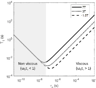
𝑏 the radius of the molecule treated as a sphere, 𝑘 is the Boltzman’s constant, and T is the absolute temperature. T1 evolution as a function of correlation time is displayed in Figure
1.2. It is now evident from Eq. (1.6) and Figure 1.2 that T1 depends on the molecular
envi-ronment considered, temperature, but also the magnetic field strength B0. If B0 increases, T1
values will increase as well, in a non-linear manner.
Much of the relaxation in biological systems takes place at relaxation sites. These are locations where magnetization energy is easily and quickly dissipated. A prime example of a relaxation site is a metal nucleus such as gadolinium (Gd). Often used as a contrast‐agent in MRI, it allows for significant shortening of the T1 by supplying a relaxation site to many spins. Other
metals such as iron (in hemoglobin) and zinc (present in many proteins) similarly act as nat-urally occurring relaxation sites (Tofts, 2005).
Figure 1.2 : Log-log representation of T1 depending on correlation time (which is proportional to vis-cosity and inversely proportional to temperature). Different magnetic field strengths are considered (line: 7T, dotted-line: 3T and dashed line: 1.5T). The T1 value depends on the molecular environment, reflected by the correlation time, 𝜏𝑐. The minimum values of the curves corresponds to 𝜔0𝜏𝑐 =1. The
shaded area corresponds to 𝜔0𝜏𝑐 < 1 at 7T, where the molecular environment is non-viscous.
There-fore, the interactions are restrained and T1 does not depend on field strength. In viscous environments, T1 varies with magnetic field strength in a non-linear manner.
Biological basis of T1
As described above, the T1 recovery is caused by the fluctuating magnetic fields arising largely
from the motion of molecules in the neighborhood of the magnetic moments. Therefore T1
relaxation is often associated with water mobility and structural density, reflecting binding of water molecules. In the brain, it has been shown to be highly correlated with myelin or mac-romolecular volume content, both in grey (Stüber et al., 2014) and white matter (Mezer et al., 2013; Yeatman et al., 2014). That is why T1 contrast is generally used in brain exams:
myelin causes white matter to have a shorter T1 than grey matter, leading to a clear contrast.
T1 can change due to pathologies. For instance, edema around tumors or inflammatory acute
MS lesions leads to an increase in T1 (Brück et al., 2004). T1 is also increased in chronic MS
lesions, probably as a result of the reduction in myelin and increase in water content. But at the rim of active MS lesions, T1 is reduced because of the presence of cellular debris which
constitute extra-relaxation centers in the fluid. Other changes, such as myelination of devel-oping brain (Paus et al., 2001), or decrease of myelination due to aging (Cho et al., 1997) can benefit from T1 quantification. An extensive review of T1 values in normal and pathological
1.1.1.3. Transverse relaxation time (T2)
The transverse relaxation time, T2, is related to the magnetization decay on the transverse
plane. Considering a simplified model where only the transverse component is considered, the Bloch equations show that after a 90° pulse, it can be expressed as:
𝑑𝑀𝑇 𝑑𝑡 = −
𝑀𝑇
𝑇2 (1.7)
Therefore, it is found that it takes the form of an exponential decay, described by:
𝑀𝑇(𝑡) = 𝑀𝑇(0) e−𝑇t2 (1.8)
Where 𝑀𝑇(0) is the transverse component at t = 0. T2 is the time required for the transverse
magnetization to fall to approximately 37% ( e−1) of its initial value, as shown in Figure 1.3.
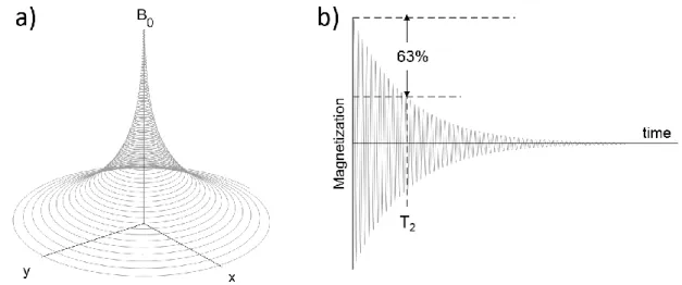
Figure 1.3 : a) Precession of the magnetization vector and b) corresponding signal, showing the T2 relaxation mechanism.
The resulting decay in transverse magnetization is due to magnetic field interactions occur-ring between protons (spin-spin interaction), slightly modifying their precession rate. For example, neighboring protons bound to macromolecules locally change the magnetic field sensed by the free protons. These local field non-uniformities cause the free protons to pre-cess at slightly different frequencies. Thus, following an excitation pulse, the protons lose phase coherence and the net transverse magnetization is gradually lost resulting in transverse magnetization decay.
As for T1, its expression can be derived from its correlation time, 𝜏𝑐, and a constant C
de-pendent on the gyromagnetic ratio and the inter-nuclear distance for proton (Nelson and Tung, 1987): 1 𝑇2 = 𝐶(3𝜏𝑐 + 5𝜏𝑐 1 + 𝜔02𝜏 𝑐2 + 2𝜏𝑐 1 + 4𝜔02𝜏 02 ) (1.9)
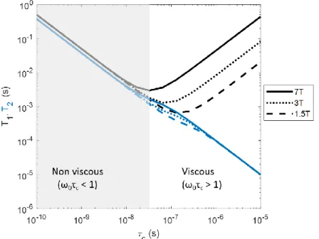
Figure 1.4 shows the T2 sensitivity on the correlation time, which is linked to the viscosity of
the environment and temperature. As illustrated, T2 values will be less sensitive to the field
strength than T1.
Figure 1.4 : Log-log representation of T1 (black lines) and T2(blue lines) depending on correlation time (which is proportional to viscosity and inversely proportional to temperature) for different magnetic field strength. Here, the dependence of T2 on magnetic field strength is less important than for T1. The molecular environment plays a pivotal role in T1 and T2 values, showing their sensitivity to probe such information.
Off-resonance effects such as imperfections in the main magnetic field, susceptibility differ-ences among various tissues or at tissue-air interfaces, and chemical shift lead to an additional dephasing of the spins and thus to a faster decay of the transverse magnetization MT. The
overall transverse relaxation time T2* , taking into account this additional reduction in
trans-verse magnetization, is determined by (Chavhan et al., 2009): 1
𝑇2∗ =
1
𝑇2 + 𝛾∆𝐵𝑖𝑛ℎ𝑜𝑚 (1.10)
Where ∆𝐵𝑖𝑛ℎ𝑜𝑚 is the magnetic field inhomogeneity, sensitive to paramagnetic mesoscopic
particles such as iron or amyloid plaques. Even with a perfect B0 shimming, T2* contains
external effects (e.g. susceptibility variations within the patient or chemical shift effects). As such, T2* is always lesser than T2. The dephasing induced by the second term of Eq (1.10)
can be eliminated by the application of an appropriate pulse (180° pulse in a spin-echo MR sequence as seen in section 2.1.2.1) which cause a reversal of the initial dephasing. In contrast, the T2 losses internal in the proton system and characteristic of the tissue are maintained as
Biological basis of T2
In the brain, T2 reflects the degree of binding and water compartmentalization. This was
evident in studies on human preterm neonates where T2 showed a decrease with brain
mat-uration (Ferrie et al., 1999). During brain matmat-uration, tissue water decreases, myelin precur-sors such as cholesterol and proteins appear, glial cells proliferate and differentiate, and a number of biochemical cell membrane changes occur. These changes increase the proportion of bound to free water and thus shorten the T2 relaxation time (Dobbing and Sands, 1973).
T1 relaxation times also decrease with cerebral maturation, particularly with the onset of
my-elination. However, T2 decreases more rapidly. Therefore, T2 has been suggested as a
partic-ularly interesting biomarker of the developing brain (Tofts, 2005).
A number of studies have shown that GM possesses a longer T2 relaxation time than WM.
This is thought to be due to differences in water compartmentalization, vascularity and iron concentration. The paramagnetic property of iron produces a shortening of the proton re-laxation times. (Vymazal et al., 1999) reported shorter T2 in regions like substantia negra, in
globus pallidus and putamen in Parkinson’s patients for example.
1.1.1.4. Proton Density
Proton density (PD) refers to the concentration of protons that resonate and give rise to the NMR signal in the tissue. It is expressed as a percentage of the proton concentration in water, in percentage unit (pu). Thus, CSF is 100pu, WM is about 70pu and GM 80pu (Tofts, 2005; Whittall et al., 1997). All images have intensity proportional to PD. Therefore, all images are PD-weighted, in addition to the influence of any other parameter such as T1 or T2 for
exam-ple. PD is sometimes called ‘spin density’ and abbreviated ρ.
Since most visible tissue protons are resident in water, it is often seen as a short-hand way of looking at water content. But PD slightly differs from water concentration. Indeed, water content would include protons that have short T2, not visible in the usual imaging process.
Significant numbers of protons are resident in non-water environments (e.g. lipids or mac-romolecules), although most of these have short T2 and are therefore MRI-invisible. But in
practice, the effect of these factors seems to be small, especially in the brain, where most mobile protons (with a long T2) are in water. (Tofts, 2005). Therefore, PD is often
approxi-mately the same as the mobile water content of the tissue.
PD is the essence of MR imaging, as it directly reflects water content as discussed above. Yet, we have little experience to measure it, and even less experience of using it clinically. PD measurements can be used to infer water content, its change in disease like inflammation and edema, and its response to treatment (e.g. mannitol to reduce edema). Changes in PD often correlate closely with T1 changes, and may provide no extra information, if T1 has
already been measured. But PD does has the advantage that its biological interpretation is unambiguous and specific. In contrast, the parameters T1 and T2, although sensitive, produce
changes that are harder to interpret. PD maps are also used to aid segmentation and tissue classification schemes, in conjunction with T1, T2 and sometimes diffusion maps (Tofts,
2005).
1.1.1.5. Diffusion
Every fluid has a characteristic intrinsic self-diffusion constant, D, which reflects the mobility of the molecules in their microenvironment. MRI can be made sensitive to dynamic displace-ments of water molecules between 10-8 and 10-4 m in a timescale of a few milliseconds to a
few seconds. Each molecule within the sample behaves independently from the others. Since these displacements are of the same order of magnitude as cellular dimensions within bio-logical tissues, MRI diffusion measurements can provide a unique insight into tissue structure and organization. Some applications like Diffusion Tensor Imaging can be used to perform fiber tracking, for example, or Intra-Voxel Incoherent Motion (IVIM) to quantitatively assess all the microscopic translational motion that could contribute to the acquired signal. Here, we will consider the mean diffusion signal encountered at the scale of a voxel.
In a free environment such as CSF, water can diffuse isotropically in all directions. In bio-logical tissues, there are barriers, such as cells and nerve fibers, which reduce the ability of water to diffuse. In the adult brain, WM and GM are characterized by structural complexity, which affects the measurements of the water diffusion coefficient in tissues. The collision between molecules provokes a random displacement of each one, with no preferred direc-tion.
When considering the NMR imaging experiment, diffusion adds a random drift to the con-sidered spins between the processes of dephasing and rephasing from gradients. The loss of phase coherence leads to a signal attenuation. The amount of diffusion attenuation depends on two factors. First, the sample structural characteristics determine the motion of the spins. Secondly, sequence parameters, where the diffusion time, td, determines the time during
which the diffusive motion takes place. Indeed, the measured diffusion depends on the time for molecules to diffuse, td, relative to the average time between two successive collisions of
a molecule and a boundary, τ. If td<<τ, most of the molecules behave as if no boundaries
If the td >>τ, any molecule is likely to encounter a boundary. This will affect the
displace-ment, and a completely restricted diffusion regime is reached. In the intermediate regime, an Apparent Diffusion Coefficient (ADC) can be estimated. Because of the dependency to the diffusion time used td, a ‘true absolute’ value of diffusion is not retrieved, but only an
appar-ent coefficiappar-ent of the system under investigation, for the chosen acquisition parameters. The contrast of the diffusion-weighted images is specific to the diffusion direction investi-gated, and can change with patient orientation. To remove these dependences, three diffu-sion-images can be obtained, each looking at diffusion along one of the three orthogonal directions (Readout, Slice and Phase encoding, respectively denoted x, y and z here). In that case, the anisotropic diffusions 𝐷𝑥, 𝐷𝑦 and 𝐷𝑧 can be retrieved, and ADC is defined as the
geometric mean of these three diffusions (Bernstein et al., 2004): 𝐴𝐷𝐶 =𝐷𝑥+𝐷𝑦+ 𝐷𝑧
3 (1.11)
This ADC value is sometimes called the “trace ADC”, as it can be considered as the trace of a diffusion tensor matrix.
Biological basis
In biological tissues, diffusing molecules are surrounded by a complex microstructural envi-ronment, unknown in detail and difficult to model, where elements such as cell membranes create partial barriers or obstacles to the molecular motion. These barriers or obstacles can restrict diffusion. The destruction of such biological barriers in disease is seen by an increase in ADC. Changes due to pathological process can modify the molecular environment and affect ADC, such as inflammation, edema, cell swelling or necrosis, membrane damage, de-myelination, and others (Tofts, 2005).
1.1.2. Clinical interests of quantitative MRI
In 1971, Damadian (Damadian, 1971) attracted the attention of the medical community by his work on tumor detection in animals using relaxation time measurements based on NMR. He was the first to report that normal and pathological tissues can be distinguished by means of relaxometry. Ever since, relaxometry has gained paramount importance and proved to fundamentally advance the diagnostic power of MRI. Indeed, abnormalities observed on weighted-imaging can be associated with multiple biological disorders. To attain a greater understanding of the natural history of the disorder, characterize the extent of tissue injury, and monitor the temporal evolution of both individual lesions and the overall disease activity, additional quantification techniques need to be employed (Tofts, 2005).
Better characterization of tissues and pathologies
The intrinsic multiparametric-dependence of MRI signal, reflecting the interactions of water molecules on a cellular level, can provide such in vivo tissue characterization. As discussed in the previous sections, the direct link between the retrieved signal and tissue properties such as PD, T1, T2 and diffusion can reflect tissue composition, allowing a direct
characteri-zation of tissues. Hence, tissue alterations can be detected with high specificity and sensitiv-ity. Quantification, being objective and bias-free, has attracted increased interest as a poten-tial biomarker for the detection of even subtle or diffuse pathological changes.
Earlier detection of pathological changes
In several studies, relaxation time measurements have demonstrated potential impact for the early diagnosis and progression monitoring of diseases in the human brain, body, and heart. Relaxation time variation in the brain has been reported in numerous contexts to improve the detection and staging of various diseases, e.g. in studies concerning autism (Deoni, 2011), dementia (Erkinjuntti et al., 1987), Parkinson’s disease (Baudrexel et al., 2010; Vymazal et al., 1999), multiple sclerosis (Larsson et al., 2005; Odrobina et al., 2005), epilepsy (Townsend et al., 2004; Liao et al., 2018), stroke (Bernarding et al., 2000), and tumors (Badve et al., 2016; Just and Thelen, 1988). Quantitative MRI can have considerable clinical value, as interven-tion or treatment could occur before neurons were irreversibly damaged or lost (Helpern et al., 2004).
In the body, measurements of transverse relaxation times (T2 and T2*) have proven value for
the assessment of iron accumulation occurring in many pathologies, e.g. in pancreas, spleen (Schwenzer et al., 2008), kidney (Schein et al., 2008), and the liver, where quantitative T2 and
T2* relaxometry has proven to be an accurate noninvasive means to measure absolute iron
content and has replaced gold-standard biopsy procedures in many centers (Cheng et al., 2012). T1 has also been investigated in the lung (Arnold et al., 2004; Jakob et al., 2001).
Fur-thermore, relaxometry is an established method for the evaluation of cartilage disease and has shown ability to detect early biochemical changes before gross morphological alterations occur (Recht and Resnick, 1998). In muscle, diffuse lesions, hardly detectable with weighted imaging become clear with quantitative MRI, comparing with normal tissues references val-ues (de Sousa et al., 2011). In cardiac applications, relaxation time measurements are benefi-cial for assessing cardiac iron overload (Ghugre et al., 2006), myocardial infarction (Van de Werf et al., 2008), edema (Giri et al., 2009), and hemorrhage (Bradley, 1993). Characterization
of atherosclerotic plaques in the main vessels has been shown to be improved when quanti-fication of T1, T2 and PD replaces qualitative assessment of the vessel walls (Yuan and
Ker-win, 2004)
Quantitative MRI has been shown necessary to improve diagnosis or prognosis, and maybe to optimize therapy planning (Higer and Bielke, 2012). Recent studies investigate the possi-bility of predicting response of tumor to treatment using tissue relaxation times; e.g. the T1
relaxation time can potentially be an indicator of chemotherapy response (Jamin et al., 2013; Weidensteiner et al., 2014). Several studies have demonstrated the utility of ADC and T2
mapping in the quantitative evaluation of prostate cancer (Boesen et al., 2015; Hambrock et al., 2011). Currently, ADC mapping is the most widely used quantitative property in the im-aging-based diagnosis and characterization of prostate disease (Yu et al., 2017). A compre-hensive review of the medical relaxometry applications is given in (Cheng et al., 2012).
Longitudinal follow-up and Multi-centric evaluations
qMRI is a promising tool to isolate particular tissue properties without the confounding in-fluence of other MR parameters. Indeed, accurate and precise measurements are made using careful techniques that take full account of all processes affecting the measurement. Deter-mination of tissue-specific parameters in a quantitative way enables to directly compare MR images across subjects for a proper follow-up. For example, in addition to providing early diagnosis, quantitative relaxometry has been used to follow cartilage repair treatment (Trattnig et al., 2011).
The quantitative results can also be compared between scanners for multi-centric evalua-tions, facilitating group comparisons. A recent example in the literature has shown that using the same sequence on different scanners with the same subject can lead to a variability of 0.8% within the human brain (Voelker et al., 2016).
1.1.3. Conclusion
We now understand the mechanisms that allow an ensemble of spins immersed in a magnetic field and excited by a RF pulse to relax back to equilibrium. These mechanisms reflect tissues properties. PD corresponds to the water content, and varies significantly in disease, although less than other parameters. More knowledge of its behavior may give important insights into biological processes underlying diseases. T1 and T2 can vary dramatically depending on
pa-thology. The possibility to perform quantitative MRI opens the possibility of an earlier de-tection of pathological changes, through a better tissue characterization of tissues. It would also make possible longitudinal intra and inter-individual follow-up, as well as multi-centric
evaluations on different scanners. Retrieving such information with a high resolution would allow a better tissue characterization and would give more insights to the clinicians to pin-point the exact diagnosis.
1.2. Enhancing MR signal using ultra-high fields strengths
With the aim of continuously improving MR images, higher magnetic field strengths are explored to obtain higher Signal-to-Noise Ratio and Contrast-to-Noise Ratio. Nevertheless, the use of these tools comes with physical constraints. Some solutions are being developed to tackle these limitations and are presented in this section.
1.2.1. The benefits to go towards higher field strengths
Signal-to-Noise Ratio
The signal in a voxel is generated from the total magnetic moment of the spins. There are different ways to enhance this signal, as shown in Equation (1.2). The inverse proportionality of M0 to the temperature T indicates that sensitivity can be enhanced at lower sample
tem-peratures. Obviously, it is unrealistic for in vivo applications. The other obvious solution comes from the linear dependence of M0 on the magnetic field strength B0. It directly implies
that higher magnetic fields improve the signal detected by the MR coil.
In the meantime, no direct relationship exists between noise and magnetic field strength. Therefore, based on Eq.(1.2), the Signal-to-Noise Ratio is expected to increase with B0. The
theory indicates that it is true in a range of intermediate field, typically around 1.5T, but seems to deviate substantially from this rule with a very high magnetic field, evolving rather supra-linearly as predicted by Ocali (Ocali and Atalar, 1998) and confirmed experimentally by Pohmann in recent works, where SNR~B01.65 (Pohmann et al., 2015).
Contrast-to-Noise Ratio
As important as having a high signal is the possibility to differentiate different neighboring tissues. Going towards more intense fields also influence relaxation times in a non-linear way, as shown in Figure 1.4. The susceptibility effects are exacerbated with magnetic field, leading to an increased sensitivity to T2* contrasts. T1 also increases in tissues with field strength, but
remain stable in liquids, as observed in Figure 1.2. Applications such as MR angiography benefits from this property, as the difference between the short T1 of blood, and the longer
Physicians have adopted the high-field imaging technology and joined in to actively partici-pate in its progress. Currently, the three major vendors have together installed more than 70 7T around the world (Polimeni and Uludağ, 2018). Siemens obtained the U.S. Food and Drug Administration (FDA) clearance as well as CE marking for a clinical 7T MRI device in October 2017, taking 7T one step closer to becoming a platform for advanced clinical imag-ing. Their installation and use for research purposes as well as clinical practice are expected to dramatically increase, as observed for 3T in the 2000’s. The objectives of such an upmarket move are multiple in radiology, ranging from a better delimitation of lesions to the demon-stration of lesions, invisible otherwise (Ge et al., 2008). Unfortunately, alongside the oppor-tunities provided by UHF MRI, several challenges arise.
1.2.2. Challenges from ultra-high field MRI
B0 heterogeneity
In areas where the difference between tissues’ susceptibility is large, such as the air-tissue interface, substantial fluctuations are introduced into the static field observed by the spins, resulting in overall image degradation. Due to the dependence of magnetization M0 on the
external field B0, these non-uniformities become more pronounced in UHF MRI, as shown
in Figure 1.5. Although these effects can be compensated with the aid of first and second-order shim coils, residual variations typically remain near intracranial cavities. These unde-sired disparities in the main field not only result in signal loss due to intra-voxel dephasing, but also in geometrical distortions originating from the bias introduced in the frequency en-coding.
Different methods are developed to mitigate these undesirable effects, in particular by the use of additional shim coils to homogenize the B0 up to higher orders. However, these are
generally not sufficient. Indeed, at 7T, the slightest respiratory or pulsatile movement can cause large fluctuations in B0, going as far as the brain. For this reason, more and more
research centers using UHF are moving towards “dynamic shimming” techniques, for exam-ple, with field probes that measure and correct these variations in real time. This subject was not in the scope of this work, but more information can be found in literature (Aghaeifar et al., 2018; Vannesjo et al., 2014).
Figure 1.5 : ΔB0 maps (in Hz) acquired at 3T (a, b) and simulated for 7T (c, d). B1 heterogeneity
UHF MRI benefits in terms of SNR and CNR are undermined by the huge disadvantage of the inhomogeneous propagation of the radiofrequency field in the human body at 297MHz. Indeed, the RF excitation of spins should be as uniform as possible to obtain a consistent contrast. The homogeneity of the B1 field comes from several elements, from which the
architecture of the coil constitutes a first factor. In addition, the electromagnetic behavior of tissues constitutes a second factor. It is mainly characterized by two properties. First, the relative permittivity of tissues, εr, characterizes the ability of atoms to move and orient under
the effect of an electric field. Secondly, their conductivity, σ, affects the resulting current density during free charge transport. It defines their ability to let electric charges move under the effect of the electric field. These quantities are related to the magnetic field and the elec-tric field by the Maxwell’s equations, governing the laws of electromagnetism (Maxwell, 1865). David Hoult (Hoult, 2000a) has shown that these dielectric properties of the human tissues are modified from 3T and above. This impacts the Maxwell equations and will affect the B1 excitation field.
Figure 1.6 illustrates the electromagnetic problem encountered at 297 MHz on a sphere as well as on the head. The B1 fields retrieved from a classic birdcage coil at this frequency in
the presence of a human head or a sphere of same permittivity show the B1 heterogeneity
Figure 1.6 : B1 field resulting from a 16-leg birdcage coil at 297MHz using CST software a) on a sphere b) on a specific anthropomorphic phantom, both filled with same permittivity and conductivity material of εr =42 and σ=0.99 S/m.
These different factors result in cancellations in certain regions during RF transmission. This leads to dark areas in the image, revealing interference phenomena called “dielectric arti-facts”(Hoult, 2000a), even when the desired flip angle α is locally attained in other regions (Van de Moortele et al., 2005) (see Figure 1.7).
Figure 1.7 : Simulated gradient echo images as a function of the magnetostatic field B0 using a bird-cage coil with ideal current distributions in the rungs. From (Webb, 2011).
Specific Absorption Rate (SAR)
For a given pulse and flip angle α, an increased energy deposition is encountered at UHF (Bottomley and Andrew, 1978; Hoult, 2000a). For a conPducting sphere of radius 𝑏 and of specific resistance 𝑅𝑆, the power dissipated in a homogeneous way is (Hoult and Lauterbur,
1979): 𝑃 =𝜋𝜔0 2𝐵 12𝑏5 15𝑅𝑆 (1.12) We can observe the quadratic relation of the power dissipated in the object with the magne-tostatic field B0 and with the field B1. This has two consequences: first, it is necessary to send
more power to obtain a sufficient field B1 at any point in the region to be imaged. Second,
more power is absorbed by the body, resulting in a rise in temperature that could lead to tissue damage.
Since the equipment is not able to directly measure the temperature generated by the coil in the tissues, limitations on the power of the transmitted RF have been established, based on the Specific Absorption Rate (SAR). International standards (IEC 60601-2-33) provide guidelines for the maximum energy deposition in human subjects to provide sufficient safety with respect to the induced temperature. These recommendations are based on the one hand on the measurement of the global SAR, that is to say the SAR induced in all the considered volume (here, the whole head) and on the other hand on the local SAR, induced in 10g of tissue. The recommendations of this standard for SAR for a human head are presented in Table 1.1.
These values are based on various scientific studies (Athey, 1989; Athey and Czerski, 1988; Barber et al., 1990) stating that temperatures of 38 °C located in the head, 39 °C in the trunk and 40 °C in the extremities, are not likely to have harmful effects. Therefore, for the head, these standards are established so that the temperature rise in the eye, an unperfused ana-tomical part, does not exceed 2°C.
10s 6min
Local SAR (10g) 20W/kg 10W/kg
Global SAR (whole head) 6,4W/kg 3,2W/kg
Table 1.1 : International SAR standards for acceptable limits for a human head based on two scales (spatial and temporal)
It turns out that, according to Hoult, (Hoult, 2000a), the evolution of the SAR as a function of the frequency and as a function of the distance in the sample is not linear. Figure 1.8 shows that for any fixed distance z, when the frequency increases, the SAR reaches a maxi-mum and then decreases. The same goes for a fixed frequency.
Figure 1.8 : Absolute value of SAR in a sphere of 10cm radius, for a B1 field applied by a quadrature coil of 5.87uT (v = 250Hz), depending on the frequency and depth in the load. (Hoult, 2000a)
Therefore, to obtain images only depending on the relaxation properties of the tissue to be analyzed, it is essential to mitigate the B1 field locally at 7T, to homogenize the spins’ flip
angle at every pixels, while taking care to not exceed SAR limitations.
1.2.3. Solutions
1.2.3.1. Dielectric pads and meta-materials
As seen in simulations (Figure 1.6 and Figure 1.7) and confirmed by images obtained on human brain in vivo at 7T, dark areas appear in the temporal lobes and in the cerebellum area when using a standard birdcage. It is necessary to modify the B1 field locally to
homog-enize the flip angle at any point in the image.
One way to do this would be to better adapt the coils to the medium to be imaged by adding materials in the coil. The study of the literature shows that this adaptation can be achieved by applying pads composed of a mixture of water and high permittivity materials on the skin of the patient (Brink and Webb, 2014; Yang et al., 2006), near the temporal lobes or in front of the cerebellum. The permittivity of the air is close to that of the vacuum whereas that of the water is much higher (≈80 at 20 °C). Replacing the air with a high permittivity material makes it possible to carry out an impedance adaptation, thus avoiding electromagnetic losses. Quantitative measurements have shown that these high permittivity pads introduced into the coil do not increase global or local SAR (Teeuwisse et al., 2012a), while significantly increas-ing the quality of the image, particularly in the temporal lobes and the cerebellum, as shown in Figure 1.9.
Figure 1.9: Images from a Turbo Spin Echo sequence (T2-weighted), without dielectric pads (first line) and with dielectric pads (second line). The white arrows show the areas particularly improved by the dielectric pads, from (Teeuwisse et al., 2012a).
Unfortunately, dielectric pads are not entirely fulfilling the requirements to be used in UHF clinical routine. They represent an important bulk in the coil, they reduce patient’s comfort, and they degrade rapidly. Some materials can be expensive and others like barium titanate (BaTiO3), referenced as toxic. To foster the RF transmission and avoid these inconveniences,
a solution based on the use of Meta-Material structures, acting like a magnetic resonators in the RF coil, has been proposed by the Institut Fresnel in collaboration with Neurospin and is currently being studied. It will be discussed in more details in Chapter 4
1.2.3.2. Parallel transmission RF static shimming
To address the origins of the problem, another solution adopted in the community is the use of parallel transmission (pTx). The coil remains a birdcage, but each rung is powered by separate amplifiers instead of a single one. The interferences of these 𝑛𝑇 transmission
chan-nels are then optimized to produce a more homogeneous RF field. In RF static shimming, the same RF pulse waveform, 𝑝(𝑡), is transmitted on each channel, scaled by a channel-specific complex weight, 𝑤𝑐, so that the sum of the fields is as homogeneous as possible,
according to the following equation:
𝐵1+(𝑟, 𝑡) = 𝑝(𝑡) ∑ 𝑤 𝑐𝑆𝑐(𝑟) 𝑛𝑇
𝑐=1
(1.13) Where 𝐵1+(𝑟, 𝑡) is the resulting field in position 𝑟 of the volume at time 𝑡, 𝑆𝑐(𝑟) is the spatial
transmit sensitivity produced by each channel, and 𝑤𝑐 is the complex coefficient (magnitude
and phase) applied to each transmitting coil to obtain a 𝐵1+(𝑟, 𝑡)as close as possible from the targeted value in every point of the region of interest.
To estimate the coefficients 𝑤𝑐, a calibration of the system is necessary. It consists in the
acquisition of B1+ maps from each of the 𝑛𝑇 channels separately, to perform an adjustment
to optimize the different 𝑤𝑐. This new degree of freedom given by such technology makes
possible the correction of a large part of the problems encountered at 3T on large organs. At higher fields, this approach unfortunately only partially solves the problems encountered.
RF dynamic shimming
Another more complex solution is to determine individually the excitation that will be ap-plied in each region of the space. Yip and colleagues have proposed a method to design pulses that satisfy this query (Yip et al., 2005). The counterpart is in very long pulses that are difficult to use in a conventional sequence pattern. Thus Grissom (Grissom et al., 2006) and
Katscher (Katscher and Börnert, 2006) have proposed an extension of this approach by tak-ing advantage of multichannel transmission systems.
In that case, it is not a static complex coefficient 𝑤𝑐 that is optimized for each transmission
channel but rather a pulse specific to each channel, 𝑝𝑐, taking into account their respective
behavior 𝑆𝑐(𝑟). We then speak of a “dynamic B1+ shimming”. This can be written:
𝐵1+(𝑟, 𝑡) = ∑ 𝑝
𝑐(t)𝑆𝑐(𝑟) 𝑛𝑇
𝑐=1
(1.14) Like static shimming, it is necessary to make a specific calibration of each of the channels according to the patient placed in the coil. To further reduce the pulses durations, more effective strategies have been proposed in recent years as was able to synthesize Padormo in a review article on the subject (Padormo et al., 2016). These solutions are very elegant but require computing time during the exam and are very complex. More recently, (Gras et al., 2017a) came up with a solution taking advantage of the reproducibility of the brain shape to provide a push-button solution, called “Universal Pulses”. Given a coil and a sequence, this solution provides a pulse applicable to any patient in the scanner, avoiding such loss of time and efficiency in clinical routines for the brain. These solutions will be discussed in more details later on in this manuscript. The application of such techniques allows to make the most of UHF, in order to obtain high-resolution quantitative images, to go further in the quantification of tissues and possible diagnosis. To perform such quantification, different strategies can be adopted, as will be presented in the next chapter.
Chapter 2. Measuring NMR parameters
Chapter 2.
Measuring NMR parameters
uantitative MRI relies on measurement of NMR parameters of interest listed in Chapter 1 in a robust manner. The measurement must not depend on any external factor, but only reflect tissue properties and environment. Different approaches have been studied to retrieve such information. In this section, we will first describe the Spin-Echo sequence, used for gold-standard measurements, and show how it is used to properly retrieve quantitative measurements. Although some acceleration strategies can be adopted, these spin-echo based solutions are still long and can hardly be applied in clinical routine at UHF. Another strategy is to use Steady-State Free Precession (SSFP) sequences, described later on in this section. As the correlation of multiple complementary NMR parameters could help in the interpre-tation of the physio-pathological events, strategies for implementing multi-parametric simul-taneous measurements in a single sequence are currently being developed in the literature, usually based on such SSFP sequences. A brief and qualitative overview of these methods will also be presented in this chapter, discussing the feasibility to apply each strategy at 7T. Finally, the objectives and challenges of this PhD thesis will be described.
2.1. Measuring NMR parameters of interest
2.1.1. Spatial encoding
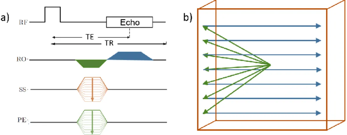
To perform imaging, the vast majority of sequence consists of a train of excitation pulses that are separated by a constant repetition time (TR). A specificity of MRI is that the images are acquired in the Fourier domain, by filling the “k-space”. This k-space encoding is per-formed between consecutive excitation pulses by means of switched magnetic gradient pulses, oriented along arbitrary X, Y and Z logical directions, called read, phase, and slice-selection directions. Their intensities vary over time in order to spatially encode the signal coming from the spins. Indeed, when considering a cluster of spins that precess with the same frequency (called an isochromat), these gradients will induce local magnetic field vari-ations, leading to a unique precession frequency for each isochromat at a distinct spatial location. This precession frequency, depending on the spatial coordinates of the spins, allows to retrieve their location. Figure 2.1 illustrates a basic chronogram of a sequence and the associated k-space sampling pattern. Different gradient-switching patterns can be used to encode the image. The most widespread sampling strategy is the use of Cartesian encoding, where regularly spaced lines (frequency encoding or readout) are acquired each TR, the or-thogonal coordinates corresponding to the incremental phase encoding steps. Other non-Cartesian methods can be applied to reduce acquisition time, but are out of the scope of this manuscript. Information can be found in (Lauterbur, 1973; Ahn et al., 1986; Pipe, 1999).
Figure 2.1: a) Chronogram of a 3D Gradient Recalled Echo (GRE) sequence and b) associated sche-matic sampling pattern in k-space. RF: Radiofrequency emission, RO: Readout gradients, SS: Slice Selection gradients, PE: Phase-Encoding gradients. Colors in the chronogram corresponds to associated displacement in the k-space.
By applying an inverse Fourier transformation, the matrix of NMR signals is reverted into an MR image in the space domain and an image is retrieved, as shown in Figure 2.2.
Figure 2.2 : Logarithm of the modulus of complex k-space NMR data (a) and the magnitude of the associated reconstructed image through 2D discrete inverse Fourier transform (b)
We now understand pulse sequence diagrams, and how images can be retrieved using MR. The very basic pulse sequence is called the “Spin-Echo” (SE) experiment, originally discov-ered by (Hahn, 1950) in spectroscopy. It is now used to perform imaging and has many variations, as described in the following section.
2.1.2. Spin-Echo sequences
2.1.2.1. Spin-echo
In the Spin-Echo experiment, a first flip angle 𝛼1 is applied to the system. Once this
excita-tion has been applied to the system, because of the presence of imaging gradients, these spin isochromats have a range of precession frequencies. Some precess faster than the Larmor frequency, while others precess slower. This produces a phase dispersion among the spin isochromats. The application of a “refocusing RF pulse” of flip angle 𝛼2 will rotate the
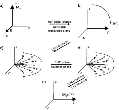
dis-persing spin isochromats about an axis in the transverse plane so that the magnetization vector will rephase (or refocus) at a later time (Haacke et al., 2014). Figure 2.3 presents a simplified picture of the behavior of the individual spins during the experiment.
Figure 2.3 : Description of spins behavior during a spin echo experiment. a) Spins are along z-axis, forming M0 vector. b) A 90° pulse rotates the spins around the x’-axis, into the transverse plane where they begin to precess. c) The spins accumulate extra phase, until d) this accumulation is inverted by the 180° refocusing pulse. The spins continue to collect extra-phase at the same rate and, at a later time, e) all spins return to the positive y’-axis together, forming a spin echo. The echo amplitude is reduced by the intrinsic T2 decay. From (Haacke et al., 2014)
An expression for the retrieved signal can be derived (Bernstein et al., 2004):
𝑆 = 𝑀0sin 𝛼1sin2( 𝛼2 2) 1 + (cos 𝛼2− 1)𝑒− 𝑇𝑅−𝑇𝐸2 𝑇1 − cos 𝛼2𝑒− 𝑇𝑅 𝑇1 1 − cos 𝛼1cos 𝛼2𝑒−𝑇𝑅𝑇1 (2.1)
If 𝑇1 ≪ (𝑇𝑅 −𝑇𝐸2), then the signal in Eq. (2.1) is maximized by setting 𝛼1=90° and
𝛼2=180°, leading to: 𝑆 ∝ 𝑀0 𝑒−𝑇𝐸𝑇2(1 − 2𝑒− 𝑇𝑅−𝑇𝐸2 𝑇1 + 𝑒− 𝑇𝑅 𝑇1) (2.2)
Therefore, to refocus transverse magnetization optimally, refocusing RF pulses commonly have a flip angle of 𝛼2 = 180°. Other values of the flip angles can be used with shorter TR
to increase the signal or to maximize the contrast between a particular pair of tissue types. Sometimes, a lower value of the flip angle of the refocusing pulse is used to reduce SAR, particularly at 3.0T and above.