From global scaling to the dynamics of individual cities

HAL Id: cea-01626240

https://hal-cea.archives-ouvertes.fr/cea-01626240

Preprint submitted on 30 Oct 2017

HAL is a multi-disciplinary open access

archive for the deposit and dissemination of

sci-entific research documents, whether they are

pub-lished or not. The documents may come from

teaching and research institutions in France or

abroad, or from public or private research centers.

L’archive ouverte pluridisciplinaire HAL, est

destinée au dépôt et à la diffusion de documents

scientifiques de niveau recherche, publiés ou non,

émanant des établissements d’enseignement et de

recherche français ou étrangers, des laboratoires

publics ou privés.

From global scaling to the dynamics of individual cities

Jules Depersin, Marc Barthelemy

To cite this version:

Jules Depersin, Marc Barthelemy. From global scaling to the dynamics of individual cities. 2017.

�cea-01626240�

Jules Depersin

Institut de Physique Th´eorique, Universit´e Paris Saclay, CEA, CNRS, F-91191 Gif-sur-Yvette, France

Marc Barthelemy∗

Institut de Physique Th´eorique, Universit´e Paris Saclay, CEA, CNRS, F-91191 Gif-sur-Yvette, France and

Centre d’Analyse et de Math´ematique Sociales, (CNRS/EHESS) 54, Boulevard Raspail, 75006 Paris, France Scaling has been proposed as a powerful tool to analyze the properties of complex systems, and in particular for cities where it describes how various properties change with population. The empirical study of scaling on a wide range of urban datasets displays apparent nonlinear behaviors whose statistical validity and meaning were recently the focus of many debates. We discuss here another aspect which is the implication of such scaling forms on individual cities and how they can be used for predicting the behavior of a city when its population changes. We illustrate this discussion on the case of delay due to traffic congestion with a dataset for 101 US cities in the range 1982-2014. We show that the scaling form obtained by agglomerating all the available data for different cities and for different years displays indeed a nonlinear behavior, but which appears to be unrelated to the dynamics of individual cities when their population grow. In other words, the congestion induced delay in a given city does not depend on its population only, but also on its previous history. This strong path-dependency prohibits the existence of a simple scaling form valid for all cities and shows that we cannot always agglomerate the data for many different systems. More generally, these results also challenge the use of transversal data for understanding longitudinal series for cities.

Keywords: Science of cities | Scaling | Path dependency

The recent availability of data for cities opens the fas-cinating possibility of a science of cities [1, 2] and has led numerous scientists to search for general laws [3, 4] ruling the evolution of various socio-economical and structural indicators such as patent production, personal income or electric cable total length, etc. In [3], it was suggested that assuming the population P to be the most impor-tant determinant for cities, we could study the evolution of many different features when P is increasing. In [4], many socio-economic factors were studied versus popula-tion indicating the existence of simple scaling laws under the form of power laws. For each indicator Y , Betten-court et al. [4] found a power law of the form Y ∼ Pβ where the exponent β depends on the quantity consid-ered. Some quantities evolve superlinearly with the popu-lation (β > 1), for instance new patents (β = 1.27), GDP (1.13 < β < 1.26) or serious crime (β = 1.16), while some other behave sublinearly (β < 1) as gasoline stations or sales. Quantities that are independent from the size of the city – typically human-related quantities such as wa-ter consumption – scale with an exponent β = 1. The usual explanation for these effects is the impact of in-teractions (scaling as P2_{) for superlinear quantities, and}

economies of scale for sublinear quantities. This publica-tion [4] was followed by a wealth of other measures such as the abundance of business categories [5], the number of sexually transmitted infection [6], road networks [7], or carbon dioxide emissions [8–12].

Scaling in urban systems has however been criticized in some recent papers [10, 13–16]. A first re-analysis of

the data for the GDP and income [13] showed that the power law could not be distinguished from other func-tional forms, or that the linear fit is better [14], and in [15] the authors led a rigorous investigation on the statis-tical quality of scalings for various quantities and found that in many superlinear cases, the linear assumption could in fact not be rejected. They also showed that the fitting results depend crucially on the assumptions about noise. From another point of view, the authors in [16] showed that, for some socioeconomic indicators, those scaling are not universal and could depend on de-tails of urban systems. More precisely, they showed on data of 5, 000 french cities that two different definitions of the cities (Unit´e urbaine (Urban Units) and Aire ur-baine (Metropolitan areas)) lead to different values of the scaling exponent for a given quantity, a result confirmed on transport-emitted CO2in [10]. Not only the value of

the exponent can change, but in some case, for different definitions of the city, the scaling regime changes: for in-stance, the number of jobs in the manufacturing sector grows superlinearly with the population of Urban Units, but sublinearly if one considers Metropolitan Areas [16]. We can expect the results to change quantitatively, but here we have changes from the superlinear to the sub-linear regime, casting some doubts about this nonsub-linear scaling and its universality.

In this paper we raise another problem that is the rel-evance of such a scaling for the individual dynamics of cities. At a more theoretical level, we question here the scaling assumption where a quantity Y (usually

2 sive) is assumed to be determined by the population only

Y = F (P ) (where F is in general an unknown function). Even if the population is an important determinant for cities we cannot exclude time effect and path-dependency which would then imply that the quantity Y depends also on time Y = F (P, t) and possibly on all Y (t0) for t0 < t. In other terms, the path-dependency means that it doesn’t make sense in general to compare two cities having the same population but at very different dates: both central Paris and Phoenix (AZ) had a population of about 1 million inhabitants, the former in 1840 and the latter in 1990, and it is very likely that the dynam-ics – for most of the relevant quantities – from 1840 in Paris will be very different from the one starting in 1990 in Phoenix, implying that the usual scaling form does not apply in general. In this paper, we investigate this question and test if a scaling exponent computed by ag-gregating data for different cities (usually at a same date) is relevant for predicting what will happen at the level of individual cities as their population grow. We illustrate this discussion on the case of congestion-induced delays but our results could have far-reaching consequences on many other scaling results for cities.

Aggregating all cities: Global scaling

We focus on the particular case of traffic congestion and its impact on time delays. Previous studies have been made in order to empirically test and theoretically explain how traffic congestion scale with the population. In [17, 18] for instance, the authors propose a theory of urban growth which accounts for some of the observed scalings. The theoretical predictions are tested against several data sets, collected by OCDE or by a GPS device company (TomTom) [17]. Here, we study the dataset (freely available at [19]) published by the Texas A&M Transportation Institute (TTI) in the Urban Mobility Report (UMR), obtained for 101 cities in the United States over 33 years (from 1982 to 2014). This database has been investigated in 2017 by [20] and in this study, the authors agglomerate all the data corresponding to different cities and performed the usual power law fit of the form

δτi = aP β

i (1)

where δτi is the annual congestion induced delay

corre-sponding to the city i. In this study we take for Pi (also

denoted by P in the following) the number of car com-muters for the city i rather than the population, because this is the relevant parameter in many models that deal with congestion in cities (see [18]). If we take the popula-tion instead of the number of car commuters, our results are qualitatively the same and our conclusions remain un-changed, even if all the exponent values change slightly (a fit for all cities and all years shows that the number

of car commuters is approximately a constant fraction of order 35% of the population). In [20], they used the least square method to estimate β and for the year 2014 (the last available year in the urban mobility report), we find with this method β = 1.23 ± 0.03. We plot the data and the corresponding fit on Fig. 1.

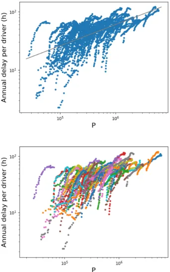
FIG. 1: Plot of the annual delay δτ versus the number of drivers P for all cities in 2014 (data from TTI’s Urban Mobility Information website, see [19]). The

straight line is a power law fit in this loglog representation and gives an exponent value β ≈ 1.23

(and R2_{= 0.93).}

The quality of a fit has in general to be carefully checked with the help of statistical methods [15], and computing a good estimation of this exponent values re-lies on several assumptions: data points are independent, the noise is multiplicative and has a variance independant of Pi (homoscedasticity). It should also be checked that

the nonlinear fit that has an additional parameter com-pared to the linear one, is much better than what would be expected by pure chance. In this case, the trend seems however to fit the data in a reasonably good way with a large R2 = 0.93, even if we have only two decades here. The value of β larger than 1 indicates a superlinear be-havior of the traffic congestion, a fact in agreement with recent empirical [20] and theoretical approaches [18, 21]. We can repeat this fit for each year separately, from 1982 to 2014. Formally, we test for each time t the re-lationship log(δτi(t)) = log(a) + β(t) × log(Pi(t)) + noise

where β(t) is the scaling exponent to determine. We show the values of β(t) versus t in Fig. 2 and we observe that β(t) is not constant through time and displays non-negligible fluctuations of order 20%. However all these values are larger than 1 indicating a consistent superlin-ear behavior. In [20] a least square method has been used on all the points available: they mix all the 33 years avail-able for each of the 101 cities and get 33 × 101 = 3333 points leading to a scaling exponent β ≈ 1.36 ± 0.01,

FIG. 2: Scaling exponent β(t) for the delay computed for each year separately, from 1982 to 2014. All these values are consistent with a superlinear behavior found

in [20].

consistent again with a superlinear relation. ,as found in [20]. For this dataset, we plot the scatterplot and the cor-responding nonlinear fit in Fig. 3(top) (note that we plot here the delay per capita). We observe some variabil-ity but the global increasing trend seems to be correct. This way of proceeding with data is common: one mixes data for different cities and for the available years, and then performs a regression over the whole set. The scal-ing that is obtained – and that we qualify as ‘global’– is then used for discussing theoretical approaches. For instance, in [21], this approach is used for computing some scaling exponents (for quantities such as land area, wages, etc.) and are compared with the exponent ex-pected from theoretical calculations. In [22], empirical regularities are found by applying this methodology to different indicators, suggesting the existence of a univer-sal socioeconomic dynamics. Beyond statistical problems related to fitting procedures, the exact meaning and the relevance of this global scaling for individual cities is how-ever not clear. In other words, when we know that a cer-tain quantity Y scales for all cities as Y ∼ Pβ, what can we say about the evolution of a single city ? In the fol-lowing we address this question on the case of congestion delay and by studying in details the dynamics of every individual city and compare its behavior with the global scaling described above.

The dynamics of individual cities

In Fig. 3(bottom), we show the same plot as in Fig. 3(top) but where we now distinguish cities (one color corresponds to one city). This allows us to compare the evolution of the delay due to congestion in each city when

FIG. 3: (Top) Scatterplot of the annual delay per capita δτ /P versus P for all the 101 cities and for all years (1982-2014). The straight line is the power law fit with

value β ≈ 1.36 consistent with a superlinear behavior. (Bottom) Same scatterplot but where the points are colored according to the city they describe (one color per city). As we discuss in the text there is no obvious

relation between the global power law scaling and the individual behavior of cities.

its population grows. The first striking observation is that for all cities in our dataset, the evolution of the con-gestion delay does not behave as predicted by the global trend. They have their own trend which depends on their particular history. In this respect, it is natural to ask what is the individual city dynamics and what does it have in common with the global scaling. In what follows we thus focus on this individual behavior and discuss its relation with the global power law exponent.

4

Absence of a single scaling

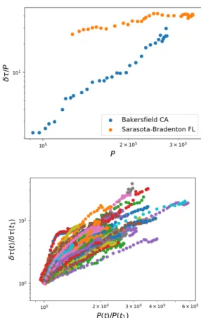
With this dataset, we can monitor the evolution of each city when its population grows. The first thing that we observe on the examples in Fig. 4(top) is that the annual delay is not a simple function of P only. The value of the number of drivers (or the population) is not enough to determine the delay. We also note in this figure that the slopes are different (a power law fit gives β ≈ 3.20 for Bakersfield and β ≈ 1.45 for Sarasota) showing that even when a power law exists it is not with the same exponent (see below for a further analysis of this point). In order to test further the existence of a scaling of the form δτ ∼ Pβ

we plot in Fig. 4(Bottom) for all cities δτ (t)/δτ (t1) versus

P (t)/P (t1) where t1 is the first available time. Even if

FIG. 4: (Top) Loglog plot of the annual delay per capita δτ /P versus P for two different cities: Bakersfield (CA) and Sarasota (FL). For the same range of P values, the delay is different, and the slopes

are different as well. (Bottom). Plot of the rescaled delay δτ (t)/δτ (t1) versus P (t)/P (t1). The curves

correspond to different cities and the fact that they do not collapse indicates the absence of a unique scaling

determined by a single exponent.

the prefactor changes from a city to another this rescaling allows to test the existence of a unique power law scaling.

As we can see in this figure 4(bottom), the curves for different cities do not collapse signalling the absence of a scaling form governed by a single exponent. In the following we will focus on the different behaviors observed for this set of cities.

Different categories of cities

We analyze the behavior of each of the 101 cities in the dataset and we observe a variety of behaviors. More precisely, there are two main categories characterized by different time evolutions:

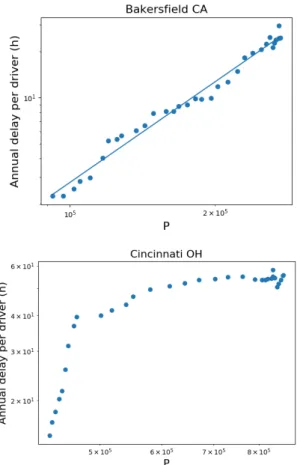
• The delay increases with P and in most cases can be fitted by a power (see Fig. 5(top)) and we refer to this set as ‘type-1’ cities and which represent over 30% of our cases. We note here that for the dataset studied here, the time range (from 1982 to 2014) does not allow to have a very large variation of the number of drivers (the ratio P (2014)/P (1982) varies from 1.2 to 6 approximately) and a much larger dataset would be needed in order to have a better accuracy for these exponent values.

• The other cities (about 40% of all cities) display two regimes separated by a change of slope that is in general abrupt. The second regime for these ‘type-2’ cities can be in some cases a ‘saturation’ where the delay stays constant. We show in Fig. 5(bottom) an example of such city that displays saturation with a zero slope in the second regime. • The rest of cities (≈ 30%) do not display a common

behavior (for instance some present 3 changes of slope, etc.)

In most cases however, the individual behavior of a city does not correspond to the global scaling δτ ∼ P1.36_{. In}

the following we focus on each of these classes and try to characterize them more precisely.

Type-1 cities: power law growth

This particular class comprises cities that display an individual scaling law that can be fitted by a power law of the form δτ (t) ' P (t)βi _{, where P (t) is the number}

of commuters at time t and δτ (t) the corresponding an-nual congestion-induced delay. The quantity βi depends

in general on the city i and we show in Fig. 6 the his-togram for this exponent computed for all type-1 cities. We clearly see that very few cities behave as the ‘global trend’ predicted: only 2 cities over 31 have an exponent < 1.5, while 13 cities have an exponent > 2.5. This re-sult shows that when we observe a power law behavior at the individual city level, it is generally with an expo-nent that is much larger than 1 and much larger than

FIG. 5: Loglog plot of the annual delay per capita δτ /P versus P from 1982 to 2014. (Top) An example of a type-1 city where the delay grows with P and that can be reasonably fitted by a power law (Bakersfield, CA). (Bottom). Example of a type-2 city with two power law

regimes characterized by two different exponents (Cincinatti, OH).

the result found for the global scaling. In other words there seems to be no correlation between the global ob-servation made on all cities and the individual behavior of cities when its population evolves.

Type-2 cities: existence of two regimes

For about 40% of the cities in the dataset, the delay versus the number of car commuters displays a change of slope and log(δτ ) is a piecewise linear function of log(P ). Formally one could write:

log(δτ ) = (

a1+ β1× log(P ) when P < P∗

a2+ β2× log(P ) when P > P∗

(2)

This behavior indicates that the dynamics of the traffic congestion in those cities followed successively two differ-ent scaling laws with two differdiffer-ent expondiffer-ents β1 and β2

and we plot the histograms for both these exponents in

FIG. 6: Empirical histogram of β for type-1 cities. The vertical line indicates the value of the global scaling

β ≈ 1.36.

Fig. 7. We note that the average of β1is around 5.3, while

FIG. 7: Empirical histograms for the two exponents β1

and β2 that describe the two regimes of type-2 cities.

(Top) Histogram for β1 and (Bottom) the histogram for

β2. For most cities we have β1> β2.

ex-6 ponent’ (but with a large dispersion around this value).

Beyond averages, we have that for almost every case, β1 > β2. Almost all the exponents of the first regime

β1 are above 2 (indicating a strong superlinearity) while

the second exponents β2 are mostly < 2. For this second

regime, some cities do not exhibit superlinear behaviour. Indeed for some cities (∼ 30%), the exponent β2 is very

close to 1, indicating a linear behavior and equivalently a delay per capita constant – that we coined ‘saturation’. The cities of Akron (see Fig. 8), or Pittsburg for instance fall into that subcategory. We also observe that in some

FIG. 8: Example of two different type-2 cities with two regimes characterized by two exponents β1 and β2. In

the case of Akron (OH) we observe a ‘saturation’ with a constant delay per capita (β2≈ 0), while for

Albuquerque (NM) the delay per capita decreases with the population (β2< 0).

cases a crossing between the curves corresponding to dif-ferent cities can occur (such as Akron and Albuquerque in Fig. 8). This crossing is another sign that the poste-rior evolution of a city is not uniquely determined by the population and the delay at a certain time (if it did the evolution after the crossing should be identical for the two cities).

In other cases (∼ 10%), the exponent β2 is clearly

< 1, which indicates sublinearity and that the delay per capita decreases with the population. We show the example of the city of Albuquerque (New Mexico) in Fig. 8. This phenomenon is very counter intuitive, even if we can point out some elements of explanation. In-deed, in addition to the congestion induced delay, we also have the data for the total driven length Ltot (in

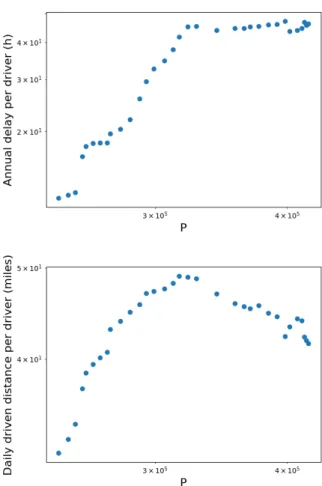
miles × commuters) for each city and each year. We can check if this quantity can explain, even partially, the be-havior of the total delay. For some type-2 cities with two regimes, we plot the driven length per commuter against the number of drivers and we observe that this curve dis-plays a change of regime at the exact same point for the delay. In Fig. 9(top), we see that for the case of

Birm-ingham, from 1998, the delay remains almost constant, whereas it increased constantly at a high rate before that (more precisely we have here β1 ' 4 and β2 ' 0).

In Fig. 9 (bottom), we observe that in the same year, the curve for Ltot/P experienced a change of slope: the

length per capita increased before 1998, and slowly de-creases after that date. This could explain partially why the delay does non evolve after this date: there are cer-tainly more people on the road after 1998, and therefore more likely some congestion, but each commuter drives less on average which decreases the occurrence of traffic jams: these two effects can compensate each other. This is one possible partial explanation, which however does not hold for all the cities. The change of slope in Ltot/P

vs P is common in this dataset and in most cases hap-pens simultaneously with the change of regimes of the delay, pointing to the existence of correlations between these quantities, even if not in a causal manner. The simultaneous change of regime for these two quantities might also be the sign that the city experienced a large scale structural change.

FIG. 9: Birmingham case. (Top) Loglog plot of δτ /P versus P . (Bottom) Loglog plot of the total driven

length per capita Ltot/P vs P .

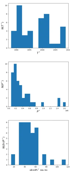
β1 and β2, we can also study (i) at what time T∗ the

change of slope happened, (ii) what was the population of the city when it happened (P∗), and (iii) what was the delay par capita when it happened ((δτ /P )∗_{). We}

repre-sent the histograms for these three quantities in Fig. 10. The distribution of T∗ is difficult to interpret and do not display a typical date at which the slope changes. The change of slopes do not occur at the same time for these cities, which would have been the case for instance if there had been a national plan in the US to rebuild the whole road system, or any other federal decision. The histogram for P∗ seems clearer to interpret with the ex-istence of a clear maximum around 200, 000 commuters and a quick decay for larger values. The average of the distribution is 394, 000, while the standard deviation is 367, 000. Finally, the delay per capita (δτ /P )∗ displays a histogram that has a relatively small compact support, with an average of about 39 hours per year, and a stan-dard deviation about 18 hours per year. This relatively small variation of (δτ /P )∗ _{suggests that it is the}

conges-tion that triggers the change of regime signalled by dif-ferent exponents. Further studies are however certainly needed in order to clarify this important point.

Discussion

We focused in this paper on the dataset for congestion-induced delay in some US cities. This is a particularly interesting dataset as it is both transversal (it contains many cities), and longitudinal (for each city we have the temporal evolution of the delay). This is a rather rare case at the moment, but this type of data will certainly become more abundant in the future and will allow to test our results on other quantities. Our observations about scaling might therefore have far reaching consequences for the quantitative study of urban systems, well beyond the case of congestion induced delays.

The general scaling form Y ∼ Pβ _{indicates that if the}

population is multiplied by a factor λ the quantity Y is then multiplied by a factor λβ_{. This scaling form}

re-lies however on a strong implicit assumption which is the ‘logarithmic population translation’ invariance. In other words, this scaling form implies that for any times t and t0 we have Y (t0)/Y (t) = (P (t0)/P (t))β and then depends on the ratio of populations only (or the differ-ence of logarithms). As we observed in this study, there is no such scaling at the individual city level but a vari-ety of behaviors. In the language of statistical physics, the quantity Y (here equal to δτ ) is not a state function determined by the population only, and displays some sort of aging effect where the delay in a city depends not only on the population but also on the time, and probably on the whole history of the city. In any case we cannot make for a given city a prediction for time t2 > t1 knowing only its state for t1. This idea of

path-FIG. 10: Empirical histograms for T∗, P∗(in unit of million inhabitants) and (δτ /P )∗. In particular the histogram for (δτ /P )∗ shows that the changes of slope

in type-2 cities appears approximately at the same value of about 40 hours per year and per capita of

congestion delay.

dependency is natural for many complex systems, and in statistical physics, we know that spin-glasses [23] for example display aging which means that some features of the system (for instance the relaxation time) evolves with the age of the system and does not depend on the state of the system only. This in particular implies that

8 we do not have time translation invariance but that most

functions of two times t and t0 do not depend on t − t0 only. This aging theory has been applied to many other complex systems, from ‘soft material’ [24] to superpara-magnet [25], and it would be interesting to understand it in the framework of the evolution of urban systems.

The results presented in this paper illustrated on the case of congestion-induced delays could in principle be applied to any other quantity. They highlight the risk of agglomerating data for different cities and to consider that cities are scaled-up versions of each other (as ques-tioned in [26] for example): there are strong constraints for being allowed to do that such as path-independence, which is apparently not satisfied in the case of congestion, and which should be checked in each case.

Beyond scaling, these results also pose the challenging problem of using transversal data (ie. for different cities) in order to get some information about the longitudinal series for individual cities. This is a fundamental prob-lem that needs to be clarified when looking for generic properties of cities.

Acknowledgments JD thanks the ENSAE and the IPhT for its hospitality.

Bibliography

∗

Electronic address: marc.barthelemy@ipht.fr [1] Batty M (2013) The new science of cities. Mit Press. [2] Barthelemy M (2016) The Structure and Dynamics of

Cities. Cambridge University Press.

[3] Pumain, D (2004) Scaling laws and urban systems. SFI Working paper: 2004-02-002.

[4] Bettencourt LMA, Lobo J, Helbing D, Kuhnert C, West GB (2007) Growth, innovation, scaling, and the pace of life in cities. Proceedings of the national academy of sci-ences (USA) 104:7301-7306.

[5] Youn H, Bettencourt LMA, Lobo J, Strumsky D, Samaniego H, West GB (2016) Scaling and universality in urban economic diversification. J. R. Soc. Interface 13: 20150937.

[6] Patterson-Lomba, O, Goldstein E, Gomez-Li´evano A, Castillo-Chavez C, Towers S (2015) Per-capita Incidence of Sexually Transmitted Infections Increases Systemati-cally with Urban Population Size: a cross-sectional study. Sexually Transmitted Infections 91:610-614.

[7] Samaniego H, Moses ME (2008) Cities as organisms: Allometric scaling of urban road networks. Journal of Transport and Land use 14;1(1).

[8] Glaeser EL, Kahn ME (2010) The greenness of cities: carbon dioxide emissions and urban development. Jour-nal of Urban Economics 67:404418.

[9] Fragkias M, Lobo J, Strumsky D, Seto KC (2013) Does size matter? Scaling of CO2 emissions and US urban areas. PloS ONE 8:e64727.

[10] Louf R, Barthelemy M (2014) Scaling: Lost in the smog. Environment and Planning B 41:767-769.

[11] Oliveira EA, Andrade Jr JS, Makse HA (2014) Large cities are less green. Scientific Reports 4:4235.

[12] Rybski, Diego, et al. (2017) Cities as nuclei of sustain-ability? Environment and Planning B: Urban Analytics and City Science 44:425-440.

[13] Shalizi CR (2011) Scaling and hierarchy in urban economies. arXiv preprint arXiv:1102.4101.

[14] Arcaute E, Hatna E, Ferguson P, Youn H, Johansson A, Batty M (2015) Constructing cities, deconstructing scaling laws. Journal of The Royal Society Interface 6;12(102):20140745.

[15] Leitao JC, Miotto JM, Gerlach M, Altmann EG (2016) Is this scaling nonlinear? Royal Society open science 3:150649.

[16] Cottineau C, Hatna E, Arcaute E, Batty M (2017) Di-verse cities or the systematic paradox of urban scal-ing laws. Computers, Environment and Urban Systems, 63:80-94.

[17] Barthelemy M (2016) A global take on congestion in ur-ban areas. Environment and Planning B: Planning and Design, 43:800-804.

[18] Louf R, Barthelemy M (2014) How congestion shapes cities: from mobility patterns to scaling. Scientific Re-ports 4:5561.

[19] http://tti.tamu.edu/documents/ums/ congestion-data/complete-data.xlsx

[20] Chang YS, Lee YJ, Choi SS (2017) Is there more traffic congestion in larger cities? -Scaling analysis of the 101 largest U.S. urban centers. Transport Policy. 59:54-63. [21] Bettencourt LMA (2013) The origins of scaling in cities.

Science, 340:1438-1441.

[22] Bettencourt LMA, Lobo J, Strumsky D, West GB (2010) Urban Scaling and Its Deviations: Revealing the Struc-ture of Wealth, Innovation and Crime across Cities. PLoS ONE 5:e13541.

[23] Bouchaud JP, Cugliandolo LF, Kurchan J, M´ezard M (1997) Out of equilibrium dynamics in spin-glasses and other glassy systems. In A P Young, editor, Spin glasses and random fields, Singapore, 1998. World Scientific. [24] Fielding SM, Sollich P, Cates ME (2000) Aging and

rhe-ology in soft materials. Journal of Rherhe-ology, 44:323-69. [25] Sasaki M, Jonsson PE, Takayama H, Mamiya H (2005)

Aging and memory effects in superparamagnets and su-perspin glasses. Physical Review B, 7;71:104405.

[26] Thisse JF (2014) The new science of cities by Michael Batty: the opinion of an economist. Journal of Economic Literature, 52:805-819.