Learning Monotonic Genotype-Phenotype Maps

Volume 10, Issue 1 2011 Article 3

and Molecular Biology

Learning Monotonic Genotype-Phenotype

Maps

Niko Beerenwinkel, ETH Zürich

Patrick Knupfer, ETH Zürich

Achim Tresch, Ludwig-Maximilians-Universität München

Recommended Citation:

Beerenwinkel, Niko; Knupfer, Patrick; and Tresch, Achim (2011) "Learning Monotonic Genotype-Phenotype Maps," Statistical Applications in Genetics and Molecular Biology: Vol. 10: Iss. 1, Article 3.

Learning Monotonic Genotype-Phenotype

Maps

Niko Beerenwinkel, Patrick Knupfer, and Achim Tresch

Abstract

Evolutionary escape of pathogens from the selective pressure of immune responses and from medical interventions is driven by the accumulation of mutations. We introduce a statistical model for jointly estimating the dynamics and dependencies among genetic alterations and the associated phenotypic changes. The model integrates conjunctive Bayesian networks, which define a partial order on the occurrences of genetic events, with isotonic regression. The resulting genotype-phenotype map is non-decreasing in the lattice of genotypes. It describes evolutionary escape as a directed process following a phenotypic gradient, such as a monotonic fitness landscape. We present efficient algorithms for parameter estimation and model selection. The model is validated using simulated data and applied to HIV drug resistance data. We find that the effect of many resistance mutations is non-linear and depends on the genetic background in which they occur.

KEYWORDS: genotype-phenotype map, conjunctive Bayesian networks, HIV drug resistance,

isotonic regression

Author Notes: A.T. was supported by an LMUexcellent guest professorship. N.B. was partially

1

Introduction

Most pathogens, including viruses, bacteria, eukaryotic parasites, and cancer cells, have a tendency to escape from selective pressure that is meant to control them. Rapid evolutionary change of the pathogen population facilitates escape from nat-ural immune responses and from medical interventions such as chemotherapy. A quantitative understanding of evolutionary escape is at the heart of designing effec-tive vaccines and treatment strategies.

The escape dynamics are governed by the space of possible genotypes that is accessible to the pathogen population, by the fitness landscape over these geno-types, and by additional population genetics parameters, such as population size and mutation rate (Iwasa, Michor, and Nowak, 2003). Here, we focus on the struc-ture of the genotype space and the fitness landscape defined on it. We develop a statistical framework to estimate this fitness landscape from observed data subject to order and monotonicity constraints.

Constraints on the order in which mutations reach fixation in a population are common to many biological systems (Weinreich, Delaney, Depristo, and Hartl, 2006, Poelwijk, Kiviet, Weinreich, and Tans, 2007, Lozovsky, Chookajorn, Brown, Imwong, Shaw, Kamchonwongpaisan, Neafsey, Weinreich, and Hartl, 2009). We represent these constraints by a partial order among mutational events. The geno-type space is the lattice of order ideals of this poset (Figure 1). For the fitness land-scape, we assume that evolution proceeds in a directed fashion following an evolu-tionary gradient. We require that whenever a genotype g precedes another genotype h, their fitness is non-decreasing, φ (g) ≤ φ (h). This assumption appears reason-able in the situations indicated above, where the pathogen is under strong selective pressure and can avoid extinction only by accumulating advantageous mutations.

In the present paper, our goal is to jointly estimate both the underlying mutational order constraints and the fitness landscape from observed genotype-phenotype data. Estimating a fitness landscape amounts to learning a mapping that assigns each genotype a non-negative fitness value, or more generally, a phenotype. Because of the monotonicity assumption that we make, the regression problem is constraint and known as isotonic regression.

The two tasks of estimating mutational dependencies and of estimating a fitness landscape have been addressed separately before. Regressing phenotype on genotype is a recurrent task, because understanding the genotype-phenotype map is a central question in biology (Sevin, DeGruttola, Nijhuis, Schapiro, Foulkes, Para, and Boucher, 2000, Reidys and Stadler, 2002, Beerenwinkel, Schmidt, Wal-ter, Kaiser, Lengauer, Hoffmann, Korn, and Selbig, 2002, Beerenwinkel, Däumer, Oette, Korn, Hoffmann, Kaiser, Lengauer, Selbig, and Walter, 2003a, Wang and Larder, 2003, Draghici and Potter, 2003, Segal, Barbour, and Grant, 2004,

Rabi-nowitz, Myers, Banjevic, Chan, Sweetkind-Singer, Haberer, McCann, and Wolkow-icz, 2006, Rhee, Taylor, Wadhera, Ben-Hur, Brutlag, and Shafer, 2006).

Estimating dependencies among mutations is also a question of general in-terest in molecular biology and genetics. Several statistical models have been pro-posed for this purpose, including Bayesian networks (Klingler and Brutlag, 1994, Deforche, Silander, Camacho, Grossman, Soares, Laethem, Kantor, Moreau, and Vandamme, 2006, Poon, Lewis, Pond, and Frost, 2007) and dependency networks (Carlson, Brumme, Rousseau, Brumme, Matthews, Kadie, Mullins, Walker, Harri-gan, Goulder, and Heckerman, 2008). Order constraints represent a specific type of dependency and a specialized Bayesian network model, called conjuctive Bayesian network (CBN), has been proposed that uses a partial order to represent these con-straints (Beerenwinkel, Eriksson, and Sturmfels, 2006, 2007, Beerenwinkel and Sullivant, 2009, Gerstung, Baudis, Moch, and Beerenwinkel, 2009).

Here, we introduce a more general statistical model based on a partially or-dered set and on isotonic regression to describe constraint and directed evolution in genotype space. We present algorithms for estimating both the poset structure and the isotonic regression function from observed data. The resulting genotype-phenotype map is optimal in the likelihood sense subject to order constraints and monotonicity. The algorithms have been implemented in the R package icbn, avail-able at www.cbg.ethz.ch/software/icbn.

The model is applied to a dataset of mutational patterns in the genome of HIV and the corresponding levels of phenotypic drug resistance of the respective viruses. We want to learn mutational order constraints that apply to the evolutionary escape of HIV from drug pressure and, at the same time, the genotype-phenotype map which assigns a resistance phenotype to each genotype and is non-decreasing in the induced genotype space.

In Section 2, we present a self-contained introduction of CBNs following Beerenwinkel et al. (2007), but with some simplifications and advancements. Sec-tion 3 is devoted to isotonic regression. In SecSec-tion 4, we combine the two models to obtain the isotonic CBN (I-CBN) model, which is further developed into the noisy I-CBN (NI-CBN) to handle measurement noise in Section 5. Section 6 re-ports performance measures of the inference algorithms based on simulated data, and in Section 7, the application of the NI-CBN model to HIV drug resistance data is presented.

2

Conjunctive Bayesian networks

We consider a fixed finite set of genetic eventsE , and assume that genetic changes are irreversible. To model the accumulation of these mutations, we define the CBN

as a triple (E ,≺,θ), where "≺" is a partial order on E , and θ = (θe)e∈E ∈ [0, 1]E is

a set of parameters. A relation e1≺ e2between two distinct events is interpreted as

event e2requiring event e1 to have happened before. A relation e1≺ e2is called a

cover relation, if for all e0∈E with e1≺ e0≺ e2, either e0= e1or e0= e2.

A subset g of events is called a genotype. The set of all possible genotypes, denotedG , is the power set of E , which is identified in a natural way with the set of all binary strings of length |E | by assigning g ⊂ E to (ge)e∈E with ge= 1 if e ∈ g,

and ge= 0 otherwise. With subset inclusion,G forms a distributive lattice. We say

that a genotype g ⊆E and a relation e1≺ e2are compatible, if (e2∈ g) ⇒ (e1∈ g)

holds. This definition extends to sets of genotypes and to sets of relations in the obvious way. The state space G(E ,≺) of the CBN model is defined as the set of all genotypes that are compatible with (E ,≺), The elements of G(E ,≺) are the order ideals of the poset (E ,≺), where an order ideal is a subset g ⊆ E that is closed downwards, i.e., if e2 ∈ g and e1 ≺ e2, then e1 ∈ g. Conversely, given any set

of genotypes G ⊆G , let (E ,≺G) be the set of all events compatible with G. Then

(E ,≺G) forms a poset, which is the unique largest poset compatible with G. For the

empty poset with no relation, we have G(E ,≺empty) =G and (E ,≺G) = (E ,≺empty

). We refer to the genotype g = /0 as the wild type, and to g =E as the completely mutated type.

For a genotype g, we denote by Exit≺(g) the set of all events that have

not yet occurred in g but could happen next. An event e ∈E might happen next if and only if e is minimal in E \ g with respect to the partial order. For e ∈ E , let θe be the conditional probability that the event e has occurred given that all

of its predecessor events have already occurred. The CBN defines the following probability distribution for the discrete random variable X with state space G(E ,≺)

Pr(X = g |E ,≺,θ) =

_∏

e∈g

θe·

∏

(1 − θe) (1)

We write CBN(E ,≺,θ) for this statistical model. The probability of observing g∈ G(E ,≺) is the probability that all the events in g have happened times the probability that none of the events that could happen next has occurred.

CBNs are Bayesian network models and they can also be defined as graph-ical models as follows. Consider the graph H with vertex setE and edges e1→ e2

for all cover relations e1 ≺ e2. The CBN model is the directed graphical model

defined by H and the probability tables

τe=      1 0 .. . ... 1 0 1 − θe θe     

Event poset Genotype lattice CBN probabilities 3 4 1 OO _??           2 __??? ???_??? ??? OO {1, 2, 3, 4} {1, 2, 3}    {1, 2, 4} ??? {1, 2} ??? _ {1}    {2} ??? /0 ???? _ θ1θ2θ3θ4 θ1θ2θ3(1 − θ4) o o o o o θ1θ2(1 − θ3)θ4 OOOOO θ1θ2(1 − θ3)(1 − θ4) OOOO _oooo θ1(1 − θ2) o o o o (1 − θ1)θ2 OOOO (1 − θ1)(1 − θ2) OOOO _oooo

Figure 1: Conjunctive Bayesian network (CBN) model. Shown is the event poset (left), the induced genotype lattice (center), and the genotype probabilities (right) of the CBN model introduced in Example 1. In the event poset, each directed edge e1→ e2stands for a relation e1≺ e2.

The entries of τe are the conditional probabilities τ_a,be = Pr(Xe = b | Xpa(e)= a),

for all a ∈ {0, 1}pa(e) and b ∈ {0, 1}, where pa(e) denotes the parents of e in H, 1 = (1, . . . , 1), and τ_1,1e = Pr(Xe= 1 | Xpa(e) = 1) = θe. The joint distribution of X

factorizes as Pr(X = g | H, τ) =

_∏

∏

_∏

_∏

_∏

_∏

because the index sets of the first, second, and last product are, respectively, g, Exit≺(g), and the empty set, for all g ∈ G(E ,≺).

Example 1. LetE = {1,2,3,4} with the relations 1 ≺ 3, 1 ≺ 4, 2 ≺ 3 and 2 ≺ 4. The lattice of order ideals of this poset consists of the seven genotypes G(E ,≺) = { /0, {1}, {2}, {1, 2}, {1, 2, 3}, {1, 2, 4}, {1, 2, 3, 4}} (Figure 1). The CBN model (E ,≺,θ) is given by the probabilities

Pr( /0) = (1 − θ1)(1 − θ2) Pr({1}) = θ1(1 − θ2) Pr({2}) = (1 − θ1)θ2 Pr({1, 2}) = θ1θ2(1 − θ3)(1 − θ4) Pr({1, 2, 3}) = θ1θ2θ3(1 − θ4) Pr({1, 2, 4}) = θ1θ2(1 − θ3)θ4 Pr({1, 2, 3, 4}) = θ1θ2θ3θ4

In the remainder of this section, we recall maximum likelihood (ML) param-eter estimation and model selection for CBNs from (Beerenwinkel et al., 2007). Let (E ,≺,θ) be a CBN model. The data for this model is a count vector n = (ng) ∈ NG,

where ng is the number of observations of genotype g. We assume throughout

the paper that each event e ∈E has been observed in at least one genotype, i.e., ∑g: e∈gng> 0. The log-likelihood function of the CBN model is

`X(θ ) =

∑

∑

∑

Proposition 1. Let (E ,≺) be a fixed poset and n ∈ NG an observed set of genotypes. The ML parameters of the CBN model(E ,≺,θ) are given by

ˆ θe=

∑g: e∈gng

∑g: below≺(e)⊆gng

, for all e∈E ,

wherebelow≺(e) = {e0∈E | e06= e and e0≺ e} is the set of events strictly below e.

Proof. See (Beerenwinkel et al., 2007, Prop. 2).

We say that a set of genotypes G ⊂G separates the events, if for any two distinct elements e1, e2∈E , there exists a genotype g ∈ G and i ∈ {1,2} such that

g∩ {e1, e2} = {ei}. It is easy to see that for G ⊂G , the relation ≺GonE is reflexive

and transitive. Furthermore, if G separates the events, then ≺G is a partial order

on E . The support of a data set n ∈ NG is defined as the set of genotypes that have actually been observed, supp(n) = {g ∈G | ng> 0}. If supp(n) does not

separate the events, then there exist events that are always observed in common. The observation of several of those events does not provide additional information. Hence non-separable events may be mapped to one event. The following result has been reported in (Beerenwinkel et al., 2007, Thm. 5). Here, we present a new and simplified proof.

Theorem 1. Let n ∈ NG be a set of observed genotypes. Ifsupp(n) separates the events, then the ML CBN model is(E ,≺_supp(n), ˆθ ), with ˆθ defined as in Proposi-tion 1 for the partial order≺_supp(n).

Proof. Recall that (E ,≺_supp(n)) is the unique largest poset compatible with supp(n). For any event poset (E ,≺) that is not compatible with supp(n), the likelihood func-tion LX(θ ) = Pr(n |E ,≺,θ) is identical zero. Thus, it is sufficient to show that if

≺1and ≺2are two partial orders onE that are compatible with supp(n) and ≺2is

larger than ≺1(i.e., for all e, e0∈E , e ≺1e0implies e ≺2e0), then the likelihood is

non-decreasing, Pr(n |E ,≺1) ≤ Pr(n |E ,≺2).

Let g ∈G be a genotype. If ≺2is larger than ≺1, then

min≺2E \ g = Exit≺2(g) ⊆ Exit≺1(g) = min≺1E \ g

To see this, suppose that e ∈E \ g is not ≺1-minimal. Then there is an element

d∈E \g with d ≺₁e. But this implies d ≺2eand hence e is not ≺2-minimal either.

For any genotype compatible with ≺_supp(n) (and hence also with ≺1 and

≺2), we find Pr(X = g |E ,≺1, θ ) =

∏

∏

_∏

∏

We assume that genotype observations are independent, hence Pr(n |E ,≺1, θ ) =

∏

_∏

(E ,≺_supp(n)) is a partial order, because supp(n) separates the events. By definition, no compatible poset can contain more relations than (E ,≺_supp(n)). Thus

Pr(n |E ,≺,θ) ≤ Pr(n | E ,≺_supp(n), θ ) ≤ Pr(n |E ,≺supp(n), ˆθ )

for any partial order ≺ and any parameter vector θ .

3

Isotonic regression

In this section, we fix a given poset (E ,≺) with genotype lattice G = G(E ,≺). We assume that the evolutionary process on G, i.e., the partially ordered accumulation

of mutations, follows a certain one-dimensional real-valued phenotype in a mono-tonic fashion. We require that the genotype-phenotype map φ : G → R satisfies for all g1, g2∈ G,

g₁⊆ g₂ ⇒ φ (g1) ≤ φ (g2)

Our goal is to estimate the unknown monotonic function φ from observed genotype-phenotype pairs (g, y) ∈ G × R.

We assume that the conditional phenotypes Y | X = g are independent nor-mal random variables with unknown means µgand common unknown variance σ2,

Y | X = g ∼ Norm(µg, σ2), for all g ∈ G

Let yg= {yg,1, . . . , yg,ng} be the phenotypes observed with genotype g. For a given

dataset (yg)g∈G, the conditional log-likelihood is

`_Y|X=g(µ, σ ) = −N 2log(2π) − N log(σ ) − 1 2σ2

∑

∑

where N = ∑g∈Gngis the total size of the data.

We estimate the parameters µ = (µg)g∈G and σ2 from the data using ML

subject to the monotonicity constraints

g1⊆ g2 ⇒ µg1 ≤ µg2, for all g1, g2∈ G (4)

This problem is known as the isotonic regression problem and its solution has the following structure. Let ¯yg= (1/ng) ∑

ng

j=1yg, j denote the average phenotype

ob-served with genotype g. For fixed σ , the ML estimates (MLEs) of µ are found by minimizing the sum of squares

∑

∑

∑

∑

subject to the constraints (4), i.e., by solving min

µ _g∈G∑ ( ¯

y_g− µg)2ng

s. t. µg1 ≤ µg2 for all g1⊆ g2in G

(5)

The optimization problem (5) is a convex quadratic programming problem with a unique local solution ˆµ which is also the global minimum. Several algorithms have been proposed for solving this constraint least squares problem (Barlow, Bartholomew, Bremner, and Brunk, 1972). In our applications, we use the R package isotone

Genotype lattice Obs. avg. phenotype (count) Predicted phenotype {1, 2, 3, 4} {1, 2, 3}    {1, 2, 4} ??? {1, 2} ??? _ {1}    {2} ??? /0 ???? _ 2.15 (6) 2.23 (3)    1.31 (7) ??? 0.98 (5) ??? _ 1.07 (4)    1.03 (5) ??? 0.03 (7) ??? _ 2.17 2.17     1.31 ???? 1.02 ???? _ 1.02     1.02 ???? 0.03 ???? _ ˆ

Figure 2: Isotonic regression on a genotype lattice. The genotype space (left) is the lattice of order ideals of the event poset shown in Figure 1. A total of 37 phenotypic measurements are summarized by their respective means and counts in the center diagram. The solution of the isotonic regression problem (5) is shown on the right, i.e., the estimated phenotypes ˆµg. See Example 2 for more details.

which implements a solution based on a convex programming formulation with lin-ear constraints and employs an active set algorithm (de Leeuw, Hornik, and Mair, 2009). The MLE of σ2is then

σ2= 1 N_g∈G

∑

∑

Example 2. For the genotype lattice of Example 1 and Figure 1, we consider the phenotype data summarized in the center diagram of Figure 2 by the average phe-notypesy¯_g and, in parenthesis, the genotype counts n_g. The MLEs of µ are found by solving the optimization problem (5). The solution is displayed on the right of Figure 2 and it has the following block structure:

ˆ µ/0 = 0.03 ˆ µ{1}= ˆµ{2}= ˆµ{1,2} = 1.02 ˆ µ_{1,2,4} = 1.31 ˆ µ_{1,2,3}= ˆµ_{1,2,3,4} = 2.17

The MLE of σ can not be computed from the average phenotypes ¯yg, but only from

the full data{yg, j} not shown in this example.

The estimated genotype-phenotype map is monotonic along any mutational pathway g1⊂ · · · ⊂ gk in G, and it has two additional properties that are important

in biological applications. First, the mapping is non-linear in the events. It allows for different phenotypic effects of the same genetic event, depending on the ge-netic context of the mutation. Second, the block structure implies that neighboring genotypes often have the same phenotype. In other words, blocks represent neutral mutational networks with respect to the considered phenotype.

4

Isotonic conjunctive Bayesian network model

We think of the observed genotype-phenotype pairs as intermediate steps of a non-reversible evolutionary process that is subject to partial order constraints and di-rected by a non-decreasing phenotype. For a fixed poset (E ,≺) with induced geno-type lattice G = G(E ,≺), we define the joint distribution of genotype-phenotype pairs (X , Y ) by the hierarchical model

X ∼ CBN(E ,≺,θ)

Y | X = g ∼ Norm(µg, σ2), g∈ G

with µg1≤ µg2 whenever g1⊆ g2in G. We call this model the Isotonic Conjunctive

Bayesian Network (I-CBN) model. For a dataset (ng, yg)g∈G, the log-likelihood

function of the I-CBN model is the sum of the CBN log-likelihood (2) and the isotonic regression log-likelihood (3), `X,Y(θ , µ, σ2) = `X(θ ) + `Y|X(µ, σ2). The

results on ML parameter estimation and model selection for CBNs extend to I-CBNs as follows.

Proposition 2. The ML parameters of the I-CBN model (E ,≺,θ, µ,σ) are given by ˆ θe = ∑g: e∈gng ∑g:below≺(e)⊆gng , for all e∈E ˆ µ = min µ

∑

∑

∑

Proof. See Proposition 1 and Section 3, and note that the partial derivatives of `X,Y

are the same as those of `X and `Y|X, respectively.

Theorem 2. Let n ∈ NG be a set of observed genotypes. Ifsupp(n) separates the events, then the ML I-CBN model is(E ,≺_supp(n),θ , ˆˆ µ , σˆ2), with ˆθ , ˆµ , and ˆσ2 de-fined as in Proposition 2 for the partial order≺_supp(n).

Proof. If (E ,≺) is not compatible with the data, then the likelihood function is zero. The poset (E ,≺_supp(n)) is the unique maximal poset that is compatible with n. Suppose there are two different compatible posets (E ,≺i), i = 1, 2, such that (E ,≺2

) is larger than (E ,≺1). Then CBN(E ,≺2) is more likely than CBN(E ,≺1) and it

suffices to shown that the isotonic regression likelihood is also non-decreasing. The data n is compatible with both posets and we have

supp(n) ⊆ G(E ,≺_supp(n)) ⊆ G(E ,≺2) ⊂ G(E ,≺1)

For any genotype g ∈ G(E ,≺1) \ G(E ,≺2), we must have ng= 0. Therefore the

log-likelihood `_Y|Xdoes not differ whether evaluated on G(E ,≺1) or G(E ,≺2).

We summarize the results of this section in the following algorithm for learning I-CBN models from data.

Algorithm 1. (Learning I-CBN models)

INPUT: A dataset(n_g, y_g)_g∈G such thatsupp(n) separates the eventsE OUTPUT: The ML I-CBN model (E ,≺supp(n),θ , ˆˆ µ , σˆ2)

STEP 1: Construct≺_supp(n)by setting, for all e₁, e2∈E , e1≺supp(n)e2

if and only if g∩ {e1, e2} 6= {e2} for all g ∈ supp(n). Set G = G(E ,≺).

STEP 2: Compute the isotonic regression (5) to obtain the MLEs ˆµ = ( ˆµg)g∈G.

STEP 3: Compute the MLEs ˆσ2and ˆθ = ( ˆθe)e∈E according to Proposition 2.

STEP 4: Output the poset(E ,≺_supp(n)) and the MLEs ( ˆθ , ˆµ , ˆσ2).

5

Error model

Algorithm 1 for learning I-CBN models using ML is appealing due its efficiency and simplicity. In practice, however, it is limited by the sensitivity of poset recon-struction (Step 1) to noise in the genotype data. A single, possibly erroneous, ob-served genotype containing e2but not e1is sufficient to remove the relation e1≺ e2

from the optimal poset.

In order to account for noisy genotype observations, we extend the I-CBN model in this section. We follow the approach of Gerstung et al. (2009) and devise an error model which assumes that the true genotype Z is generated by the CBN model, but not directly observable, and that the observed genotype X is an erroneous copy of Z,

Pr(X | Z) = εd(X ,Z)(1 − ε)n−d(X,Z)

where ε is the per-locus probability of a measurement error and d the Hamming distance between genotypes, i.e., the number of genetic events that occurred in exactly one of the two genotypes. We denote this error model by Err(Z, ε).

The model for (X ,Y, Z) is defined hierarchically as Z ∼ CBN(E ,≺,θ)

X | Z ∼ Err(Z, ε)

Y | Z ∼ Norm(µZ, σ2) with µg1≤ µg2 for all g1⊆ g2

The observed genotype X is independent of the observed phenotype Y given the true unobserved genotype Z. The noisy I-CBN (NI-CBN) model is defined as the marginalization of this model with respect to the unobserved data Z.

For fixed (E ,≺), G = G(E ,≺), and data {(xi, yi, zi)}i=1,...,N, the

complete-data log-likelihood of the NI-CBN model is

`X,Y,Z(θ , ε, µ, σ2) = `Z(θ ) + `X|Z(ε) + `Y|Z(µ, σ2) (6)

Hence the MLEs are given in Proposition 2 and by ˆε = [1/(N|E |)]∑N_i=1d(xi, zi).

The observed-data log-likelihood is

`X,Y(θ , ε, µ, σ2) = N

∑

_∑

In order to maximize this expression, we derive an Expectation Maximization (EM) algorithm (Dempster, Laird, and Rubin, 1977).

The posterior of the hidden data Z given the observations (X ,Y ) is Pr(Z | X ,Y ) = Pr(Z) Pr(X | Z) Pr(Y | Z)

∑Z0Pr(Z0) Pr(X | Z0) Pr(Y | Z0)

(7) Let γi,g= Pr(Zi= g | X ,Y ) denote the responsibility of genotype g ∈ G for

observa-tion (xi, yi). Then, for all g ∈ G,

u_{g= EZ|X,Y} " N

∑

∑

is the expected genotype count, where δ is the Kronecker delta function. This defines the E step.

For the M step, we estimate the model parameters by maximizing the ex-pectation of the complete-data log-likelihood (6) with respect to the conditional

distribution (7). We obtain the following equations for updating the model parame-ters: θ_enew = ∑g:e∈g u_g ∑g: e∈below≺(e)⊆gug , e∈E εnew = 1 N|E | N

∑

∑

∑

∑

∑

∑

where the responsibilities are computed with the previous parameter estimates. For model selection, i.e., finding the optimal poset structure, we employ simulated annealing (Kirkpatrick, Gelatt, and Vecchi, 1983), a heuristic search strat-egy, to find the ML poset. The poset space is sampled by modifications of relations of the current poset that result in a new poset. In each step, we allow for adding or removing a relation, or replacing two relations e1 ≺ e2 ≺ e3 by e1 ≺ e2 and

e₁≺ e3. To speed up the procedure, we use the number of incompatible genotypes

|G \ G(E ,≺new)| as a filter to discard unpromising poset structures prior to

likeli-hood computation (Gerstung et al., 2009).

6

Simulation study

We analyzed the performance of the simulated annealing algorithm in simulation experiments. Predicted posets were compared to the true posets in terms of the false positive rate (fpr), defined as the number of estimated false relations divided by |E |(|E | − 1)/2 (the maximum number of possible relations), and the false neg-ative rate (fnr), defined as the number of true relations not included in the esti-mated poset divided by the number of true relations. Using the cross-validated mean squared error (MSE) ∑g[φ (g) − ˆφ (g)]2, the NI-CBN model was compared to

a baseline regression model that is linear in the events E . We report the relative MSE difference, ∆MSE= (MSElinear− MSENI−CBN)/ MSElinear.

We analyzed six posets: two empty posets and two linear posets, each of size |E | = 4 and 7, the poset of Example 1 shown in Figure 1, and the poset displayed in Figure 3A which was selected based on real data (see Section 7). For each poset, we investigated models with parameters ε ∈ {0.001, 0.01, 0.1} and σ ∈ {0.1, 1} by drawing N = 500 or 1000 samples. For the empty and the linear posets, the

Table 1: NI-CBN performance for empty posets. Symbols are defined in the main text. False positive rate (fpr) and false negative rate (fnr) are reported with their standard error (se). In the penultimate column, p is the p-value of a one-sided paired Wilcoxon rank sum test of the MSE of the NI-CBN model versus the linear model, based on the number of simulations given in the last column.

|E | ε σ N fpr ± se fnr ± se ∆MSE log10p runs

4 0.001 0.1 500 0 0 0.146 –17.7 100 4 0.001 0.1 1000 0 0 0.147 –17.7 100 4 0.001 1 500 0 0 0.106 –16.7 100 4 0.001 1 1000 0 0 0.139 –17.6 100 4 0.01 0.1 500 0 0 0.114 –17.7 100 4 0.01 0.1 1000 0 0 0.125 –17.7 100 4 0.01 1 500 0 0 0.121 –17.4 100 4 0.01 1 1000 0 0 0.119 –17.6 100 4 0.1 0.1 500 0 0 0.048 –17.5 100 4 0.1 0.1 1000 0 0 0.041 –17.7 100 4 0.1 1 500 0.007±0.003 0 0.029 –6.8 100 4 0.1 1 1000 0.003±0.002 0 0.029 –11.8 100 7 0.001 0.1 500 0.005±0.002 0 0.027 –6.5 50 7 0.001 0.1 1000 0.002±0.001 0 0.054 –9.3 50 7 0.001 1 500 0.040±0.003 0 0.001 –0.4 50 7 0.001 1 1000 0.017±0.003 0 0.008 –0.4 50 7 0.01 0.1 500 0.004±0.002 0 0.028 –6.0 50 7 0.01 0.1 1000 0 0 0.036 –8.7 50 7 0.01 1 500 0.040±0.003 0 0.002 –0.3 50 7 0.01 1 1000 0.018±0.003 0 -0.005 0.0 50 7 0.1 0.1 500 0.020±0.003 0 -0.008 0.0 50 7 0.1 0.1 1000 0.003±0.002 0 0.000 –0.2 50 7 0.1 1 500 0.045±0.003 0 -0.003 –0.3 50 7 0.1 1 1000 0.034±0.003 0 -0.008 –0.1 50

conditional probabilities θ were set such that all genotypes g ∈ G(E ,≺) have the same probability, θeempty= 1/2 for all e ∈E , and θ_ilinear= i/(i + 1) for linear posets

1 ≺ 2 ≺ 3 ≺ · · · ≺ |E |. For the poset of Example 1, equal genotype probabilities can not be achieved and θ was drawn uniformly from the interval (0.5, 0.9). For the poset of Figure 3A the fitted values θ = (0.42, 0.40, 0.18, 0.59, 0.69, 0.87, 0.65) were used. The parameters µ of the NI-CBN model were generated by drawing uniform random numbers ri, i = 1, . . . , |E | − 1, from the interval (−1,3), sorting

Table 2: NI-CBN performance for linear posets. Symbols are defined in the main text and in the legend of Table 1.

|E | ε σ N fpr ± se fnr ± se ∆MSE log10p runs

4 0.001 0.1 500 0 0 0.002 –4.1 100 4 0.001 0.1 1000 0 0 0.003 –14.3 100 4 0.001 1 500 0 0 0.002 –2.7 100 4 0.001 1 1000 0 0 0.003 –8.3 100 4 0.01 0.1 500 0 0.002±0.002 0.024 –17.5 100 4 0.01 0.1 1000 0 0 0.023 –17.7 100 4 0.01 1 500 0 0.003±0.003 0.024 –16.0 100 4 0.01 1 1000 0 0 0.025 –17.6 100 4 0.1 0.1 500 0.008±0.004 0.112±0.021 0.081 –17.3 100 4 0.1 0.1 1000 0.002±0.002 0.058±0.014 0.085 –17.7 100 4 0.1 1 500 0.012±0.004 0.130±0.020 0.086 –17.6 100 4 0.1 1 1000 0.002±0.002 0.073±0.017 0.084 –17.7 100 7 0.001 0.1 500 0 0.004±0.002 0.003 –12.0 100 7 0.001 0.1 1000 0 0 0.002 –14.9 100 7 0.001 1 500 0 0.010±0.003 0.004 –9.5 100 7 0.001 1 1000 0 0.003±0.003 0.003 –11.7 100 7 0.01 0.1 500 0 0.015±0.006 0.024 –17.7 100 7 0.01 0.1 1000 0 0.002±0.002 0.022 –17.7 100 7 0.01 1 500 0 0.020±0.006 0.025 –16.6 100 7 0.01 1 1000 0 0.001±0.001 0.020 –17.5 100 7 0.1 0.1 500 0.026±0.003 0.550±0.016 0.062 –17.6 100 7 0.1 0.1 1000 0.024±0.003 0.517±0.015 0.062 –17.7 100 7 0.1 1 500 0.040±0.005 0.514±0.017 0.069 –16.5 100 7 0.1 1 1000 0.039±0.004 0.488±0.016 0.067 –17.3 100

them as −1 = r0< r1< · · · < r|E |−1< r|E |= 3, and setting µg= r|g|. This defines a

graded fitness landscape, i.e., the fitness (or phenotype) depends only on the number of mutations (Beerenwinkel et al., 2006). The runtime for fitting each model was between one minute and two hours on a standard PC.

For the empty posets (Table 1), false negatives can not occur. False positive rates were generally small and always below 5%. For the linear posets (Table 2), false positive rates are comparably low, but the false negative rate can reach high levels, especially for high error rates ε = 0.1 and small sample sizes N = 500. Sim-ilar poset reconstruction performance was observed for the poset of Example 1 and for the poset of Figure 3A with somewhat increased false positive rates (Table 3). In

Table 3: NI-CBN performance for the poset of Example 1 (4 events) and the poset of Figure 3A (7 events). Symbols are defined in the main text and in the legend of Table 1.

|E | ε σ N fpr ± se fnr ± se ∆MSE log10p runs

4 0.001 0.1 500 0.003±0.002 0 0.078 –17.6 100 4 0.001 0.1 1000 0.002±0.002 0 0.074 –17.7 100 4 0.001 1 500 0.002±0.002 0.003±0.003 0.079 –16.5 100 4 0.001 1 1000 0.010±0.004 0 0.072 –16.2 100 4 0.01 0.1 500 0.007±0.003 0 0.084 –17.7 100 4 0.01 0.1 1000 0.005±0.003 0 0.090 –17.6 100 4 0.01 1 500 0.007±0.003 0 0.082 –16.0 100 4 0.01 1 1000 0.003±0.002 0 0.085 –17.6 100 4 0.1 0.1 500 0.042±0.008 0.063±0.018 0.073 –17.5 100 4 0.1 0.1 1000 0.040±0.008 0.028±0.012 0.077 –17.7 100 4 0.1 1 500 0.085±0.013 0.143±0.022 0.065 –17.6 100 4 0.1 1 1000 0.058±0.011 0.053±0.015 0.059 –17.7 100 7 0.001 0.1 500 0.001±0.001 0.014±0.004 0.084 –17.7 100 7 0.001 0.1 1000 0 0.003±0.002 0.076 –17.7 100 7 0.001 1 500 0.007±0.002 0.017±0.005 0.052 –12.5 100 7 0.001 1 1000 0.003±0.002 0.007±0.003 0.055 –16.3 100 7 0.01 0.1 500 0.011±0.003 0.029±0.006 0.077 –17.7 100 7 0.01 0.1 1000 0.003±0.002 0.004±0.002 0.073 –17.7 100 7 0.01 1 500 0.014±0.003 0.027±0.006 0.052 –15.3 100 7 0.01 1 1000 0.002±0.001 0.004±0.002 0.083 –17.3 100 7 0.1 0.1 500 0.082±0.008 0.543±0.023 0.041 –15.1 100 7 0.1 0.1 1000 0.090±0.009 0.404±0.023 0.052 –16.3 100 7 0.1 1 500 0.130±0.011 0.566±0.023 0.040 –10.7 100 7 0.1 1 1000 0.118±0.011 0.499±0.025 0.047 –14.8 100

general, poset reconstruction is increasingly difficult for larger posets, higher error rates ε, and smaller sample size N, while the impact of the phenotype variance σ2 appears to be small (Tables 1–3).

For most posets and parameter constellations, the NI-CBN model signifi-cantly outperformed the linear model in terms of the MSE of predicted phenotypes. This was not the case only for some of the models defined by the empty poset on seven events, which was also the most difficult model to fit (Table 1). This expected superiority of the NI-CBN model confirms that linear models are not appropriate for many types of fitness landscapes.

7

Application to HIV drug resistance

We consider genetic changes in the HIV genome in response to drug therapy and an-alyze two dataset obtained from the Stanford HIV Drug Resistance Databse (Rhee, Gonzales, Kantor, Betts, Ravela, and Shafer, 2003). The first dataset consists of 617 observations of the HIV reverse transcriptase (RT) genotype and paired measure-ments of phenotypic resistance to the RT inhibitor zidovudine. Resistance levels are reported as the logarithm of the fold-change in susceptibility of the virus to the drug as compared to the wild type. The genetic events are the amino acid changes E = {41L, 67N, 69D, 70R, 210W, 215Y, and 219Q}, where, for example, 41L stands for the occurrence of leucine (L) at position 41 of the HIV RT. These muta-tions are known to be involved in the development of zidovudine resistance (Shafer and Schapiro, 2008).

The poset of the ML NI-CBN found by simulated annealing is shown in Fig-ure 3A. It exhibits two independent mutational pathways, one involving mutations 41L and 215Y, the other 67N and 70R, that have been described before (Boucher, O’Sullivan, Mulder, Ramautarsing, Kellam, Darby, Lange, Goudsmit, and Larder, 1992, Larder, 1994). In previous work, a more restrictive model class of tree posets was not able to find the independence of both pathways, but a much more complex mixture model of tree posets was (Beerenwinkel, Rahnenführer, Däumer, Hoff-mann, Kaiser, Selbig, and Lengauer, 2005). The model applied here offers more structural flexibility with the same number of free model parameters and it inte-grates both genotypic and phenotypic data into a single model.

The induced genotype lattice G(E ,≺) and the predicted drug resistance lev-els are visualized in Figure 3B and listed in the Appendix (Table 4). The lattice con-sists of 28 genotypes and the estimated isotonic regression function groups these into twelve genotype blocks of identical resistance to zidovudine. This description of the evolutionary process is much simpler than considering all |G | = 27= 128 combinatorially possible genotypes. The model suggests that under the selective pressure of zidovudine, neutral networks of neighboring genotypes of (near) iden-tical fitness exist.

Linear regression of zidovudine resistance on the genetic events E was slightly less accurate than the NI-CBN predictions with a MSE of 0.45 ± 0.024 versus 0.44 ± 0.025 as estimated by 10-fold cross-validation (p = 0.053, one-sided, paired Wilcoxon rank sum test). Despite the comparable predictive performance, the two models have a very different structure. The NI-CBN model allows for non-linear effects of mutations and for context dependancy, whereas in the linear model, the effect per mutation is averaged over all genetic contexts. For the zi-dovudine data, the linear model tends to underestimate resistance in genotypes with few mutations and to overestimate resistance when many mutations have occurred

(Appendix, Table 4). (A) _{210W 219Q} 215Y OO 70R OO 69D 41L OO 67N __???? _ ?? (B) 0000000 0100000 0101000 0101001 0110000 0111000 0111001 1000000 1000010 1000110 1100000 1100010 1100110 1101000 1101001 1101010 1101011 1101110 1101111 1110000 1110010 1110110 1111000 1111001 1111010 1111011 1111110 1111111

Figure 3: Cover relations of the optimal poset (A) and induced genotype lattice (B) for the development of HIV resistance to the nucleotide RT inhibitor zidovu-dine. Genotypes are encoded as binary strings that refer to the seven amino acid substitutions 41L, 67N, 69D, 70R, 210W, 215Y, and 219Q in the RT gene. The predicted levels of phenotypic resistance are color-coded (blue = fully susceptible, red = highly resistant). Further details, including the remaining model parameters and confidence intervals are given in the Appendix, Table 4 and Table 5.

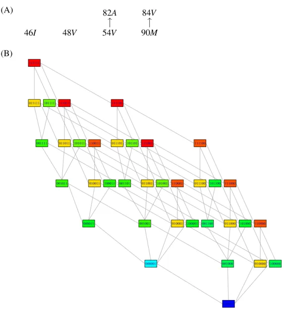
(A) _{82A 84V} 46I 48V 54V OO 90M OO (B) 000000 000001 000011 001000 001001 001011 001100 001101 001111 010000 010001 010011 011000 011001 011011 011100 011101 011111 100000 100001 100011 101000 101001 101011 101100 101101 101111 110000 110001 110011 111000 111001 111011 111100 111101 111111

Figure 4: Cover relations of the optimal poset (A) and induced genotype lattice (B) for the development of HIV resistance to the PR inhibitor indinavir. Genotypes are encoded as binary strings that refer to the six amino acid substitutions 46I, 48V, 54V, 82A, 84V, and 90M in the PR gene. The predicted levels of phenotypic resistance are color-coded (blue = fully susceptible, red = highly resistant). Further details, including the remaining model parameters and confidence intervals are given in the Appendix, Table 7 and Table 8.

parameters θ , µ, σ , and ε were re-estimated from 100 bootstrap samples. The resulting 95% confidence intervals are given in the Appendix, Tables 4 and 5. An-other 100 bootstrap samples were used to quantify the uncertainty in estimating the model structure. In Table 6, the abundance of each cover relation (or equivalently, of each edge in the Bayesian network) among the 100 optimal posets is shown. This analysis strongly supports the optimal poset of Figure 3. The only appreciable uncertainty of the model structure that we detected is the order in which mutations 41L and 215Y occur. The data appears to favor the relation 41L ≺ 215Y, but it also provides some support for 215Y ≺ 41L, which indicates that both single mutants are almost equally likely to occur.

The second dataset consists of 1473 genotypes defined on the resistance-associated amino acid substitutions E = {46I, 48V, 54V, 82A, 84V, 90M} in the HIV protease (PR) and paired measurements of resistance to the PR inhibitor indi-navir (Shafer and Schapiro, 2008). The optimal poset contains only two relations, inducing a genotype lattice of size 36 (Figure 4). The NI-CBN model groups these genotypes into 13 blocks of identical resistance levels (Appendix, Table 7). Again, the effect of several mutations appears to depend on the genetic background in which they occur. Because the linear regression model can not capture these depen-dencies, it is outperformed by the NI-CBN model in terms of MSE (0.27 ± 0.013 versus 0.25 ± 0.013, p = 0.003). All model parameters and their bootstrap confi-dence intervals are given in the Appendix, Tables 7 and 8. The structural uncertainty about the optimal poset is summarized in Table 9 of the Appendix, emphasizing the general stability of the poset while suggesting the cover relation 82A ≺ 54V as an alternative to 54V ≺ 82A, although with less than half the bootstrap support.

8

Conclusions

We have introduced a statistical model for jointly estimating the dynamics of ac-cumulating mutations in a population and the associated phenotypic changes. The I-CBN model is a CBN model coupled with isotonic regression. It estimates con-straints on the order in which mutations occur by a poset and the genotype-phenotype map (or fitness landscape) by a monotonic function. Parameter estimation and model selection are straightforward and efficient for this model. The NI-CBN model accounts for noisy observations and we have presented an EM algorithm for parameter estimation in this setting. For model selection, we propose a stochastic search procedure and we have implemented a simulated annealing algorithm.

We assessed the uncertainty associated with model estimation using the bootstrap. For the fixed optimal model structure shown in Figure 3, the model

on posets (Beerenwinkel et al., 2007, Beerenwinkel and Sullivant, 2009, Gerstung et al., 2009), tree posets or mixtures of trees (Beerenwinkel et al., 2005), and general Bayesian networks (Deforche et al., 2006). It can also be regarded as a model for regressing viral resistance phenotype on genotype. The isotonic regression model on the genotype lattice applied here combines the ability of non-linear models to account for context specificity with model interpretability.

Estimating drug resistance and the probability of evolutionary escape have been shown to improve predictions of clinical outcomes of antiretroviral therapy (Beerenwinkel, Lengauer, Däumer, Kaiser, Walter, Korn, Hoffmann, and Selbig, 2003b, Altmann, Beerenwinkel, Sing, Savenkov, Däumer, Kaiser, Rhee, Fessel, Shafer, and Lengauer, 2007). The NI-CBN model estimates both quantities jointly, and thus, will be a natural choice for enhancing clinical response predictions.

The monotonic block structure of the regression function highlights two features of evolutionary escape from drug pressure: the process is directed towards increasing levels of resistance and genotype blocks of identical resistance pheno-type indicate connected neutral networks. Evolutionary escape may thus include neutral mutations within blocks and selectively advantages mutations that cause the transition to a new block. A similar drift-and-shift pattern of evolutionary escape from immune pressure has been described for Influenza A virus (Koelle, Cobey, Grenfell, and Pascual, 2006, van Nimwegen, 2006).

The NI-CBN model presented here can offer new insights into the structure of mutational pathways and the dynamics of evolutionary escape. In the future, the model might be improved in several ways. For example, large genetic event sets can not be handled with the current algorithms and often a pre-selection is necessary. The number of model parameters grows linearly with the lattice size, which in turn can be at worst exponential in the number of events. This raises the issue of overfitting of the regression function, and additional regularization may be beneficial. On the other hand, additional parameters could make the model more flexible and allow for better fitting of the obsevred data. For example, we have chosen to model phenotypic variance by a single parameter σ for all genotypes in order to keep the total number of model parameters small and because there was no obvious reason to believe that this term differs between genotypes. In principle, however, one can assume different variance parameters σg for each genotype g.

Similarly, more detailed error models are conceivable that account separately for false positive and false negative observations (Beerenwinkel and Drton, 2007), or explicitly model the error process of the measuring device.

The model has been tested on simulated data and applied to paired genotype-phenotype HIV drug resistance data. The NI-CBN model generalizes earlier efforts to estimate dependencies among HIV mutations from genotype data alone based

Appendix

Table 4: HIV RT genotype lattice for zidovudine; see Figure 3. Data Linear model NI-CBN model

g ng y¯g φˆg uˆg µˆg 95% CI Block 0000000 196 -0.09 -0.07 241.6 -0.06 [-0.13, 0.04] 1 0100000 5 0.13 0.39 14.2 0.13 [-0.06, 0.54] 2 0110000 0 NA 0.62 3.3 0.13 [-0.06, 0.54] 2 1000000 17 0.21 0.34 13.9 0.15 [-0.08, 0.81] 3 1000010 34 0.71 0.78 43.1 0.80 [0.63, 1.02] 4 0101000 24 0.99 0.84 26.1 1.00 [0.61, 1.21] 5 0101001 35 0.97 1.09 57.1 1.00 [0.77, 1.28] 5 0111000 0 NA 1.07 0.9 1.00 [0.65, 2.23] 5 1000110 50 1.23 1.16 74.2 1.23 [1.01, 1.41] 6 1100000 1 1.60 0.80 1.9 1.30 [0.04, 1.69] 7 1100010 8 1.31 1.25 11.7 1.30 [0.97, 1.69] 7 1110000 0 NA 1.03 0.2 1.30 [0.04, 1.69] 7 1110010 6 1.03 1.48 4.6 1.30 [0.94, 1.69] 7 1100110 52 1.67 1.63 49.5 1.67 [1.49, 2.09] 8 1101000 7 2.13 1.25 5.3 1.67 [1.19, 2.05] 8 1101010 7 1.08 1.70 6.9 1.67 [1.19, 2.05] 8 1101110 7 1.29 2.08 9.0 1.67 [1.49, 2.09] 8 0111001 18 1.55 1.31 15.1 1.83 [1.20, 2.28] 9 1101001 11 1.77 1.50 8.2 2.06 [1.47, 2.48] 10 1101011 2 1.62 1.94 4.0 2.06 [1.53, 2.56] 10 1101111 7 2.11 2.32 8.4 2.06 [1.66, 2.61] 11 1110110 14 2.00 1.86 13.8 2.24 [1.88, 2.47] 12 1111000 1 2.86 1.48 0.9 2.24 [1.38, 2.69] 12 1111001 1 2.16 1.72 1.0 2.24 [1.91, 2.73] 12 1111010 0 NA 1.93 0.2 2.24 [1.38, 2.69] 12 1111011 0 NA 2.17 0.1 2.24 [1.97, 2.78] 12 1111110 1 0.62 2.30 0.7 2.24 [1.89, 2.69] 12 1111111 0 NA 2.55 1.3 2.24 [1.97, 2.87] 12

Although we have restricted our applications here to the development of HIV drug resistance, we expect the NI-CBN model to be useful also for other pathogens and for modeling the genetic progression of cancer, where the events may range from single nucleotide variants to large-scale genomic rearrangements.

Table 5: Parameter estimates and their 95% bootstrap confidence intervals for the zidovudine NI-CBN model displayed in Figure 3. The estimates for the parameters µgare shown in Table 4.

Parameter MLE 95% CI θ41L 0.42 [0.37, 0.46] θ67N 0.40 [0.35, 0.43] θ69D 0.17 [0.13, 0.24] θ70R 0.59 [0.53, 0.67] θ210W 0.69 [0.60, 0.75] θ215Y 0.88 [0.82, 0.93] θ219Q 0.65 [0.57, 0.74] σ2 0.33 [0.18, 0.41] ε 0.047 [0.039, 0.059]

Table 6: Bootstrap analysis of the structural stability of the zidovudine NI-CBN model displayed in Figure 3. The entry with row index mutation e and colum index mutation f denotes the number of times the relation e ≺ f appeared as a cover relation (or equivalently, the edge e → f appeared in the graph of the Bayesian network model) among 100 bootstrap samples. Numbers in bold face indicate the presence of the corresponding edge in the optimal ML poset of Figure 3.

41L 67N 69D 70R 210W 215Y 219Q 41L 0 3 7 0 37 60 1 67N 0 0 77 72 0 1 12 69D 0 0 0 0 0 0 1 70R 0 7 4 0 0 1 94 210W 1 0 6 0 0 0 1 215Y 34 0 5 1 67 0 0 219Q 0 1 14 2 0 0 0

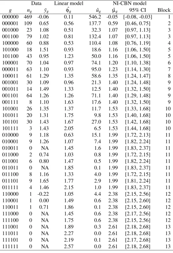
Table 7: HIV PR genotype lattice for indinavir; see Figure 4. Data Linear model NI-CBN model

g n_g y¯_g φˆg uˆg µˆg 95% CI Block 000000 469 -0.06 0.11 546.2 -0.05 [-0.08, -0.03] 1 000001 109 0.65 0.56 137.7 0.59 [0.46, 0.75] 2 001000 23 1.08 0.51 32.3 1.07 [0.97, 1.13] 3 001100 79 1.02 0.81 132.4 1.07 [0.97, 1.13] 3 100000 60 0.88 0.53 110.4 1.08 [0.76, 1.19] 4 101000 18 1.51 0.93 18.6 1.16 [1.06, 1.50] 5 101100 43 0.95 1.23 50.0 1.16 [1.06, 1.50] 5 100001 70 1.04 0.97 74.1 1.20 [1.10, 1.38] 6 000011 63 1.10 0.93 95.0 1.23 [1.14, 1.30] 7 100011 61 1.29 1.35 58.6 1.35 [1.24, 1.47] 8 001001 30 1.09 0.96 21.3 1.40 [1.24, 1.48] 9 001011 14 1.49 1.33 12.5 1.40 [1.32, 1.50] 9 001101 64 1.26 1.26 71.1 1.40 [1.29, 1.48] 9 001111 8 1.10 1.63 17.6 1.40 [1.32, 1.50] 9 101001 26 1.35 1.37 11.7 1.53 [1.33, 1.68] 10 101011 20 1.31 1.75 9.8 1.53 [1.40, 1.68] 10 101101 30 1.43 1.67 27.0 1.53 [1.42, 1.68] 10 101111 3 1.43 2.05 6.5 1.53 [1.44, 1.68] 10 010000 9 1.18 0.63 15.1 1.99 [1.72, 2.13] 11 010001 9 1.26 1.07 7.4 1.99 [1.82, 2.24] 11 010011 0 NA 1.45 1.6 1.99 [1.83, 2.37] 11 011000 2 0.74 1.03 0.8 1.99 [1.72, 2.15] 11 011001 6 0.80 1.47 0.5 1.99 [1.82, 2.24] 11 011011 0 NA 1.85 0.1 1.99 [1.83, 2.37] 11 011100 8 1.16 1.33 4.0 1.99 [1.72, 2.15] 11 011101 9 1.65 1.77 2.9 1.99 [1.81, 2.24] 11 011111 4 1.46 2.15 1.0 1.99 [1.83, 2.37] 11 110000 1 -0.22 1.05 4.4 2.38 [2.15, 2.56] 12 110001 1 0.00 1.49 0.6 2.38 [2.15, 2.60] 12 110011 1 0.71 1.86 0.1 2.38 [2.15, 2.60] 12 111000 0 NA 1.45 0.6 2.38 [2.17, 2.56] 12 111100 0 NA 1.75 0.6 2.38 [2.15, 2.56] 12 111001 0 NA 1.89 0.3 2.61 [2.18, 2.68] 13 111011 0 NA 2.27 0.0 2.61 [2.18, 2.68] 13 111101 0 NA 2.19 0.1 2.61 [2.17, 2.68] 13 111111 0 NA 2.57 0.0 2.61 [2.18, 2.68] 13

Table 8: Parameter estimates and their 95% bootstrap confidence intervals for the zidovudine NI-CBN model displayed in Figure 4. The estimates for the parameters µgare shown in Table 7.

Parameter MLE 95% CI θ46I 0.25 [0.23, 0.28] θ48V 0.03 [0.02, 0.04] θ54V 0.29 [0.26, 0.31] θ82A 0.74 [0.67, 0.79] θ84V 0.36 [0.32, 0.41] θ90M 0.38 [0.34, 0.41] σ2 0.12 [0.09, 0.13] ε 0.077 [0.068, 0.085]

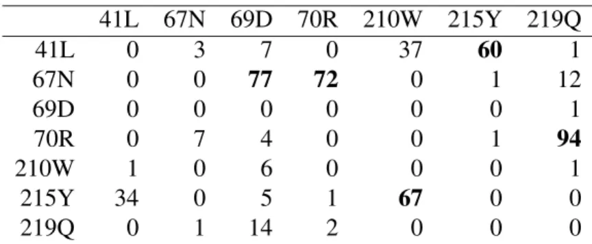
Table 9: Bootstrap analysis of the structural stability of the indinavir NI-CBN model displayed in Figure 4. The entry with row index mutation e and colum index mutation f denotes the number of times the relation e ≺ f appeared as a cover relation (or equivalently, the edge e → f appeared in the graph of the Bayesian network model) among 100 bootstrap samples. Numbers in bold face indicate the presence of the corresponding edge in the optimal ML poset of Figure 4.

46I 48V 54V 82A 84V 90M 46I 0 2 0 0 4 0 48V 0 0 0 0 0 0 54V 0 1 0 69 0 0 82A 0 4 31 0 0 0 84V 0 0 0 0 0 0 90M 2 3 0 0 81 0

References

Altmann, A., N. Beerenwinkel, T. Sing, I. Savenkov, M. Däumer, R. Kaiser, S.-Y. Rhee, W. J. Fessel, R. W. Shafer, and T. Lengauer (2007): “Improved prediction of response to antiretroviral combination therapy using the genetic barrier to drug resistance.” Antivir Ther, 12, 169–178.

Barlow, R. E., D. J. Bartholomew, J. M. Bremner, and H. D. Brunk (1972): Statis-tical Inference under Order Restrictions, John Wiley & Sons.

Beerenwinkel, N. and M. Drton (2007): “A mutagenetic tree hidden Markov model for longitudinal clonal HIV sequence data.” Biostatistics, 8, 53–71, URL http: //dx.doi.org/10.1093/biostatistics/kxj033.

Beerenwinkel, N., M. Däumer, M. Oette, K. Korn, D. Hoffmann, R. Kaiser, T. Lengauer, J. Selbig, and H. Walter (2003a): “Geno2pheno: Estimating pheno-typic drug resistance from HIV-1 genotypes.” Nucleic Acids Res, 31, 3850–3855. Beerenwinkel, N., N. Eriksson, and B. Sturmfels (2006): “Evolution on distributive lattices.” J Theor Biol, 242, 409–420, URL http://dx.doi.org/10.1016/j. jtbi.2006.03.013.

Beerenwinkel, N., N. Eriksson, and B. Sturmfels (2007): “Conjunctive Bayesian networks,” Bernoulli, 13, 893–909.

Beerenwinkel, N., T. Lengauer, M. Däumer, R. Kaiser, H. Walter, K. Korn, D. Hoff-mann, and J. Selbig (2003b): “Methods for optimizing antiviral combination therapies.” Bioinformatics, 19 Suppl 1, i16–i25, iSMB 2003.

Beerenwinkel, N., J. Rahnenführer, M. Däumer, D. Hoffmann, R. Kaiser, J. Selbig, and T. Lengauer (2005): “Learning multiple evolutionary pathways from cross-sectional data.” J Comput Biol, 12, 584–598, URL http://dx.doi.org/10. 1089/cmb.2005.12.584.

Beerenwinkel, N., B. Schmidt, H. Walter, R. Kaiser, T. Lengauer, D. Hoffmann, K. Korn, and J. Selbig (2002): “Diversity and complexity of HIV-1 drug resis-tance: a bioinformatics approach to predicting phenotype from genotype.” Proc Natl Acad Sci U S A, 99, 8271–8276, URL http://dx.doi.org/10.1073/ pnas.112177799.

Beerenwinkel, N. and S. Sullivant (2009): “Markov models for accumulating mu-tations,” Biometrika, 96, 645–661.

Boucher, C. A., E. O’Sullivan, J. W. Mulder, C. Ramautarsing, P. Kellam, G. Darby, J. M. Lange, J. Goudsmit, and B. A. Larder (1992): “Ordered appearance of zi-dovudine resistance mutations during treatment of 18 human immunodeficiency virus-positive subjects.” J Infect Dis, 165, 105–110.

of CTL escape and codon covariation in HIV-1 Gag.” PLoS Comput Biol, 4, e1000225, URL http://dx.doi.org/10.1371/journal.pcbi.1000225. de Leeuw, J., K. Hornik, and P. Mair (2009): “Isotone optimization in R:

Pool-adjacent-violators algorithm (PAVA) and active set methods,” Journal of Statisti-cal Software, 32, 1–24, URL http://www.jstatsoft.org/v32/i05

Carlson, J. M., Z. L. Brumme, C. M. Rousseau, C. J. Brumme, P. Matthews, C. Kadie, J. I. Mullins, B. D. Walker, P. R. Harrigan, P. J. R. Goulder, and D. Heckerman (2008): “Phylogenetic dependency networks: inferring patterns

.

Deforche, K., T. Silander, R. Camacho, Z. Grossman, M. A. Soares, K. V. Laethem, R. Kantor, Y. Moreau, and A.-M. Vandamme (2006): “Analysis of HIV-1 pol sequences using Bayesian networks: implications for drug resistance.” Bioinfor-matics, 22, 2975–2979.

Dempster, A., N. Laird, and D. Rubin (1977): “Maximum likelihood from incom-plete data via the EM algorithm (with discussions),” J R Statist Soc B, 39, 1–38. Draghici, S. and R. B. Potter (2003): “Predicting HIV drug resistance with neural

networks.” Bioinformatics, 19, 98–107.

Gerstung, M., M. Baudis, H. Moch, and N. Beerenwinkel (2009): “Quantifying cancer progression with conjunctive Bayesian networks.” Bioinformatics, 25, 2809–2815, URL http://dx.doi.org/10.1093/bioinformatics/btp505. Iwasa, Y., F. Michor, and M. A. Nowak (2003): “Evolutionary dynamics of escape

from biomedical intervention.” Proc Biol Sci, 270, 2573–2578, URL http:// dx.doi.org/10.1098/rspb.2003.2539.

Kirkpatrick, S., C. D. Gelatt, and M. P. Vecchi (1983): “Optimization by simu-lated annealing.” Science, 220, 671–680, URL http://dx.doi.org/10.1126/ science.220.4598.671.

Klingler, T. M. and D. L. Brutlag (1994): “Discovering structural correlations in alpha-helices.” Protein Sci, 3, 1847–1857, URL http://dx.doi.org/10. 1002/pro.5560031024.

Koelle, K., S. Cobey, B. Grenfell, and M. Pascual (2006): “Epochal evo-lution shapes the phylodynamics of interpandemic influenza A (H3N2) in humans.” Science, 314, 1898–1903, URL http://dx.doi.org/10.1126/ science.1132745.

Larder, B. A. (1994): “Interactions between drug resistance mutations in human immunodeficiency virus type 1 reverse transcriptase.” J Gen Virol, 75 ( Pt 5), 951–957.

Lozovsky, E. R., T. Chookajorn, K. M. Brown, M. Imwong, P. J. Shaw, S. Kam-chonwongpaisan, D. E. Neafsey, D. M. Weinreich, and D. L. Hartl (2009): “Stepwise acquisition of pyrimethamine resistance in the malaria parasite.” Proc Natl Acad Sci U S A, 106, 12025–12030, URL http://dx.doi.org/10.1073/ pnas.0905922106.

Poon, A. F. Y., F. I. Lewis, S. L. K. Pond, and S. D. W. Frost (2007): “An evolutionary-network model reveals stratified interactions in the V3 loop of the HIV-1 envelope.” PLoS Comput Biol, 3, e231, URL http://dx.doi.org/10. 1371/journal.pcbi.0030231.

Poelwijk, F. J., D. J. Kiviet, D. M. Weinreich, and S. J. Tans (2007): “Empirical fitness landscapes reveal accessible evolutionary paths.” Nature, 445, 383–386, URL http://dx.doi.org/10.1038/nature05451.

Rabinowitz, M., L. Myers, M. Banjevic, A. Chan, J. Sweetkind-Singer, J. Haberer, K. McCann, and R. Wolkowicz (2006): “Accurate prediction of HIV-1 drug re-sponse from the reverse transcriptase and protease amino acid sequences using sparse models created by convex optimization.” Bioinformatics, 22, 541–549, URL http://dx.doi.org/10.1093/bioinformatics/btk011.

Reidys, C. M. and P. F. Stadler (2002): “Combinatorial landscapes,” SIAM Review, 44, 3–54.

Rhee, S.-Y., M. J. Gonzales, R. Kantor, B. J. Betts, J. Ravela, and R. W. Shafer (2003): “Human immunodeficiency virus reverse transcriptase and protease se-quence database.” Nucleic Acids Res, 31, 298–303.

Rhee, S.-Y., J. Taylor, G. Wadhera, A. Ben-Hur, D. L. Brutlag, and R. W. Shafer (2006): “Genotypic predictors of human immunodeficiency virus type 1 drug resistance.” Proc Natl Acad Sci U S A, 103, 17355–17360, URL http://dx. doi.org/10.1073/pnas.0607274103.

Segal, M. R., J. D. Barbour, and R. M. Grant (2004): “Relating HIV-1 sequence variation to replication capacity via trees and forests,” Stat Appl Genet Mol Biol, 3, 2.

Sevin, A. D., V. DeGruttola, M. Nijhuis, J. M. Schapiro, A. S. Foulkes, M. F. Para, and C. A. Boucher (2000): “Methods for investigation of the relationship be-tween drug-susceptibility phenotype and human immunodeficiency virus type 1 genotype with applications to AIDS clinical trials group 333.” J Infect Dis, 182, 59–67.

Shafer, R. W. and J. M. Schapiro (2008): “HIV-1 drug resistance mutations: an updated framework for the second decade of HAART,” AIDS Rev, 10, 67–84. van Nimwegen, E. (2006): “Influenza escapes immunity along neutral networks.”

Science, 314, 1884–1886, URL http://dx.doi.org/10.1126/science. 1137300.

Wang, D. and B. Larder (2003): “Enhanced prediction of lopinavir resistance from genotype by use of artificial neural networks,” J Infect Dis, 188, 653–660. Weinreich, D. M., N. F. Delaney, M. A. Depristo, and D. L. Hartl (2006):

“Darwinian evolution can follow only very few mutational paths to fitter pro-teins.” Science, 312, 111–114, URL http://dx.doi.org/10.1126/science. 1123539.