HAL Id: hal-01083246
https://hal.inria.fr/hal-01083246v2
Submitted on 25 Jun 2015
HAL is a multi-disciplinary open access
archive for the deposit and dissemination of
sci-entific research documents, whether they are
pub-lished or not. The documents may come from
teaching and research institutions in France or
abroad, or from public or private research centers.
L’archive ouverte pluridisciplinaire HAL, est
destinée au dépôt et à la diffusion de documents
scientifiques de niveau recherche, publiés ou non,
émanant des établissements d’enseignement et de
recherche français ou étrangers, des laboratoires
publics ou privés.
Distributed under a Creative Commons Attribution - NonCommercial - ShareAlike| 4.0
Accurate computation of single scattering in
participating media with refractive boundaries
Nicolas Holzschuch
To cite this version:
Nicolas Holzschuch. Accurate computation of single scattering in participating media with refractive
boundaries. Computer Graphics Forum, Wiley, 2015, 34 (6), pp.48-59. �10.1111/cgf.12517�.
�hal-01083246v2�
Accurate computation of single scattering
in participating media with refractive boundaries
N. Holzschuch†
(a) Our algorithm (169 s) (b) Point sampling [WZHB09] (27 samples, 170 s)
(c) Photon mapping (650 000 photons, 167 s)
(d) bidirectional path tracing (520 samples per pixel, 171 s) Figure 1: Single scattering: comparison between our algorithm and existing methods (equal computation time) on a translucent sphere illuminated by a point light source from behind. For Bi-Directional Path-Tracing, we replaced the point light source with a sphere so the algorithm actually produces a picture (its angular size is ≈ 3.2◦
). Abstract
Volume caustics are high-frequency effects appearing in participating media with low opacity, when refractive interfaces are focusing the light rays. Refractions make them hard to compute, since screen locality does not correlate with spatial locality in the medium. In this paper we give a new method for accurate computation of single scattering effects in a participating media enclosed by refractive interfaces. Our algorithm is based on the observation that although radiance along each camera ray is irregular, contributions from individual triangles are smooth. Our method gives more accurate results than existing methods, faster. It uses minimal information and requires no precomputation or additional data structures.
Categories and Subject Descriptors (according to ACM CCS): I.3.7 [Computer Graphics]: Three-Dimensional Graphics and Realism—Color, shading, shadowing and texture
1. Introduction
Light traversing participating media interacts with it, being either scattered or absorbed by the medium. Combined with light concentration from occlusion or refractive interfaces,
† INRIA Grenoble - Rhône-Alpes and LJK CNRS / Université de Grenoble
scattering results in high frequency effects, such as “god rays” or underwater caustics.
Observing these effects from outside the participating me-dia adds another refractive interface between the camera and the media. This distorts the scattering effects, resulting in beautiful but challenging to render effects as shown in Fig-ure1. The two refractive interfaces between the light source
and the camera make it difficult to find light paths going from the light source to the camera after exactly one scattering event.
In this paper, we focus on objects enclosed by a refractive interface defined by triangles with interpolated vertex nor-mals, a representation close to ubiquitous in computer graph-ics. For a given camera ray, refracted at the interface, the ra-diance is equal to the integral of rara-diance received along this ray and scattered in the camera direction. This out-scattered radiance varies quickly along the ray, making it difficult to compute the integral accurately. We observe that the radi-ance caused by an individual triangle on the surface varies smoothly; discontinuities correspond to triangle edges.
We exploit this property in a new algorithm for comput-ing scomput-ingle scattercomput-ing effects with refractive interfaces. For each triangle on the surface, we quickly identify whether it is making a contribution to this specific camera ray, and on which segment of the ray. We then sample regularly inside this segment. Our method works for highly tesselated ob-jects and is significantly faster than existing methods while providing better quality results. It has been designed to be easily inserted into existing renderers, with minimal mod-ifications. It does not require additional data structures or pre-processing.
We review previous work on single and multiple scatter-ing in the next section. We describe our algorithm in details in Section3. We study the behaviour of our algorithm and compare with previous work in Section4. Finally, we con-clude and present avenues for future work in Section5.
2. Previous work
Pegoraro and Parker [PP09] provided an analytical solution for single scattering from a point light source in an homo-geneous participating media. Their approach is useful for scenes filled with smoke or dust, with no refractive inter-faces.
Volume caustics are caused by light being refracted at the interface between the refracted media and air. The most striking examples are caustics in turbid water. Nishita and Nakamae [NN94] described an algorithm to compute these caustics by creating a light shaft for each triangle on the sur-face, then accumulating the contributions from these light shafts using the accumulation buffer. Iwasaki et al. [IDN01] improved the method by using color blending between ver-tex values inside the light shaft. Ernst et al. [EAMJ05] fur-ther improved the light shaft method using non-planar shaft boundaries and computing illumination inside the shaft with fragment shaders. All these work focused on a single refrac-tive interface, displaying volume caustics as seen from inside the media.
Hu et al. [HDI∗
10] traced light rays inside the participat-ing media, after up to two specular events (reflections or re-fractions). They accumulate radiance from these light rays in
a second step. Their method produces volume caustics inter-actively, but with no refractive interface between the camera and the volume caustics.
Ihrke et al. [IZT∗
07] presented a method to compute light transport in refractive objects by modelling the propagation of the light wavefront inside the object. Their method is in-teractive and handles objects made of inhomogeneous mate-rials. It relies on a voxelised representation of light distribu-tion inside the object. Sun et al. [SZS∗
08] also used a vox-elized representation of light inside the object, but computed scattered light using photon propagation. For both methods, the resolution of the voxel grid limits the spatial resolution of volume caustics.
Sun et al. [SZLG10] introduced the line space gathering method. They first trace rays from the light source and store them as points in Plücker coordinates. Then, for each camera ray, they find the closest light rays using Plücker space and compute their scattering contributions. Their technique pro-duces high quality results, both inside and outside translu-cent objects, taking into account refraction. The data struc-tures used to store camera and light rays in Plücker space uses approximately 400 MB.
Walter et al. [WZHB09] used a Newton-Raphson iterative method to find all paths connecting a sample point inside the participating media to the light source through a refractive interface. They place sample points along camera rays in-side the translucent object to compute volume caustics. They used a position-normal tree to cull triangles in the search. Our method can be seen as an extension of theirs; we re-move the need for additional data structure and place sample points optimally for each triangle.
Jarosz et al. [JZJ08] introduced the beam radiance es-timatefor efficient rendering of participating media with photon mapping. It starts as conventional volumetric pho-ton mapping, storing phopho-tons inside the participating media. In the gathering step, camera rays are represente as beams, gathering contributions from all photons around the beam. The technique was later extended to photon beams, by Jarosz et al. [JNSJ11]: light entering the participating media is also stored as a beam of light. In the gathering step, they compute contributions from light beams to camera beams, as well as from photons to camera beams. Progressive photon beams, by Jarosz et al. [JNT∗
11], extends this idea by using beams of varying width in successive rendering steps.
3. Single scattering computations
We consider an object, filled with an homogenous partici-pating media, of refractive index η, mean free path `= σ−1
T ,
albedo α and phase function p (see Figure2). The bound-ary of the translucent object is a smooth dielectric interface. We assume that it is modelled as triangles with interpolated vertex normals.
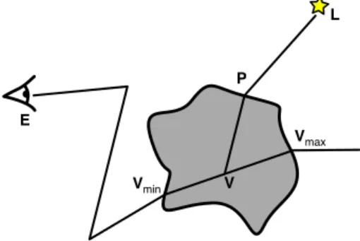
E L P V Vmin Vmax
Figure 2: We consider a translucent object, under illumina-tion from a light source L. We isolate a segment from the camera path crossing the object, and compute single scatter-ing effects on this segment.
P f Ns V L ωL ωV H ˆ ˆ ˆ ˆ
Figure 3: At point P, we define the half-vector bH, and com-pare it with the shading normal bNs. Our goal is to find zeros
of the function f=bH+bNs.
have a camera path, made of several connected segments. We take one of these segments, crossing through the translucent object, from an entry point Vminto an exit point Vmax.
We also take a point sample L on the light source: either its position for a point light source, or a random sample for an area light source.
Our goal is to compute the integral of single scattering effects from L on this specific segment of the camera path. This contribution will be combined with other lighting ef-fects computed by the renderer.
3.1. Point sampling algorithm
First, we briefly review the algorithm of Walter et al. [WZHB09]. They place several sample points V along each camera ray. For each sample point, they compute all paths connecting V to the light source L (see Section3.1.1), then compute their contribution and sum them (see Sec-tion3.1.2). For clarity, we reuse their notations.bv is a nor-malized vector:bv= v/kvk.
3.1.1. Iterative search for light paths
Given an individual triangle with interpolated vertex nor-mals, a sample point V and a light source sample L the prob-lem is to find all paths connecting L to V while following Snell’s law. The key idea is to transform this into the search for zeros of a function f. Given a point P on the triangle, with shading normal bNS, we define the normalized half-vector bH
and the function f (see Figure3):
dV = kV − Pk (1) dL = kL − Pk (2) b ωV = (V − P)/dV (3) b ωL = (L − P)/dL (4) H = ηbωV+bωL (5) b H = H/kHk (6) f(P) = bH+bNS (7)
All points P such that f(P) = 0 correspond to a path con-necting V and L, with the refraction angle following Snell’s law.
To find the zeros of f, Walter et al. [WZHB09] used a Newton-Raphson iterative method, with one small change: since point P on the triangle uses barycentric coordinates (a, b), f is a function from R2into R3. The Jacobian J of f
is a non-square matrix and thus not invertible. They used the pseudo-inverse of J, J+:
J+= (J|J)−1
J| (8)
The iterative Newton-Raphson method becomes: Pn+1= Pn− J+f(Pn) (9)
For this specific problem, it converges rapidly to a solution. 3.1.2. Contribution from each path
Once a path connecting V and L has been found, its contri-bution to the pixel is computed:
contribution= IeFAp
D (10)
where Ieis the intensity of the light source sample L, F is the
Fresnel factor at the entry point Vminand exit point P, A is
the volume attenuation (the integral of e−σTxalong [V
minV]
and [VP]), p is the phase function at V and D is the distance correction factor.
In the absence of participating media and refractive in-terface, D is the square of the distance between V and L, D= kL − Vk2= (d
V+ dL)2. With refractive media and
con-stant geometric normal bNg, D has a simple expression:
D= (dV+ ηdL) |bωL· bNg| | b ωV· bNg| dV+ |bωV· bNg| | b ωL· bNg| dL (11) With shading normals, D has a more complicated expres-sion, based on ray differentials at the interface [Ige99]. To
compute D, Walter et al. take two vectors perpendicular to ωV and each other: u⊥and uk, then compute how L changes
when ωV is perturbed along these vectors. D is the
cross-product of these derivatives: D= dL du⊥ ×dL duk (12) A complete expression of D can be found in [WZHB09]. We refer the interested readers to this article for more informa-tion.
3.1.3. Pruning triangles
The Newton-Raphson method converges with few iterations for each sample point V and each triangle. In theory, the search should be done for all triangles and all sample points, but that would be too costly. Walter et al. [WZHB09] used several methods to prune the triangles used in the search: • Sidedness agreement: V must be in the negative
half-space of the triangle, and L in the positive half-half-space, for both the geometric normal bNgand the shading normal bNs.
• Spindle test: the angle between the incoming and the re-fracted ray is betweenπ
2+ arcsin(1/η) and π. For a given
segment [VL], this restricts the potential solutions P to in-side a surface of revolution around [VL], called the spin-dle.
The spindle test doesn’t depend on triangle normals and can be used to prune large parts of the scene. For the sidedness agreement, Walter et al. [WZHB09] used a position-normal tree built from the triangles upward.
Together, these pruning methods reduced the computation time to something acceptable, a few minutes on a 8-core Xeon.
3.1.4. Numerical issues
The algorithm described by Walter et al. [WZHB09] con-verges quickly for objects made of flat triangles and moder-ately curved surfaces. The authors reported numerical issues for more complex scenes such as the bumpy sphere (see Fig-ure1):
• They have to place more samples V along each camera ray, up to 128 samples for the bumpy sphere,
• Some samples had extremely large values, which resulted in noise in the picture. These values had to be clamped in order to reduce the noise.
Our experimental study (Section3.2.1) explains these nu-merical issues: the function being integrated is highly irreg-ular, with many spikes (see Figure5). Sample points, placed randomly or regularly, are likely to miss the spikes. If one sample point happens to hit a narrow spike, it will receive disproportionate importance.
V
L
P
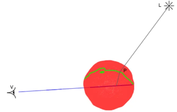
Figure 4: The set of points P corresponding to a refracted camera ray inside the object defines a curve (in green) on the surface.
3.2. Our algorithm
3.2.1. Motivation: study of a single camera ray
For a better understanding of single scattering effects with refraction, we ran an experimental study of radiance along a single camera ray. It is refracted as it enters the translu-cent object, then travels in a straight line until it exits the object. We placed a large number of sample points V along the refracted camera ray. The set of corresponding points P defines a curve on the surface of the object (see Figure4). This curve is implicitly defined by f= 0. It is irregular and can be made of several disconnected components: it is piece-wise continuous.
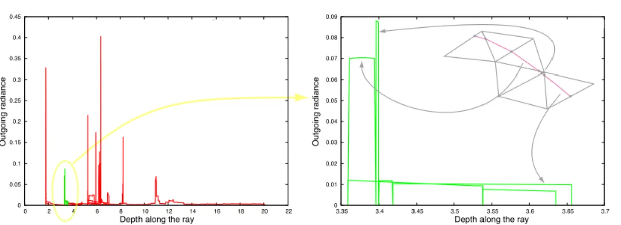
Figure5, left, shows the radiance reaching the camera for all sample points along the ray, taking into account atten-uation, phase function and ray differentials. It is highly ir-regular, with many spikes of high value, defined on a small interval.
Zooming in on a small part of this curve (Figure5, right), we observe that it is a combination of slowly varying con-tributions, with sharp discontinuities. These discontinuities correspond to triangle boundaries. This our key observation: the contribution from a single triangle to the outgoing radi-ance is a smooth function; discontinuities occur only as the curve enters and exits the triangle.
Several triangles can be contributing to the same sample point on the refracted ray: there is not a one-to-one mapping between the ray and the curve. For all points on the interval on Figure5, right, there are at least two triangles connecting this point.
Note that the spikes do not correspond to an infinite amount of light over an infinitely small sampling area, but to a very large, but finite, amount of light over a small, but measurable, area. Despite the name “volume caustics”, these are not, technically, caustics, since they are not points of in-finite energy.
0 0.05 0.1 0.15 0.2 0.25 0.3 0.35 0.4 0.45 0 2 4 6 8 10 12 14 16 18 20 22 Outgoing radiance
Depth along the ray
Radiance over ray Radiance over ray
0 0.01 0.02 0.03 0.04 0.05 0.06 0.07 0.08 0.09 3.35 3.4 3.45 3.5 3.55 3.6 3.65 3.7 Outgoing radiance
Depth along the ray
Figure 5: (left) Outgoing radiance, measured along a refracted ray inside the material. The radiance values are highly irregular: computing the integral accurately would requires many samples. If we isolate contributions from each triangle (right), each of them is smooth. Discontinuities occur only at the triangle boundaries.
f = 0 a = 0
b = 0 a+b = 1
Figure 6: f= 0 defines a curve in the triangle plane, param-eterized by t. We search for intersections between this curve and the triangle (defined in barycentric coordinates).
all sample points, the area under the curve on Figure 5, left. Smooth parts of the curve (e.g. from depth = 12 to depth= 20) can contribute more than all the spikes together. But the spikes are making it difficult for point sampling method: to avoid noise, the number of samples should be inversely proportional to the minimum width of the spikes. 3.2.2. Interval analysis along the ray
Based on this observation, the key idea of our algorithm is the following:
For each individual triangle, identify the limits of its contribution on the [Vmin, Vmax] segment, using
Newton-Raphson iterative methods. Once we have these limits, sample only inside the interval. This reduces the number of samples required.
We use the same function f defined in Equations1to7, but with a third parameter, t, the depth of point V along the re-fracted ray. t is limited in range by the entry and exit points,
Vminand Vmax, corresponding to tminand tmaxrespectively:
V= Vmin+ t
Vmax− Vmin
kVmax− Vmink
(13) f is now a function of three parameters: t and the barycen-tric coordinates (a, b) of point P on the triangle plane. f= 0 is a polynomial equation of degree 6 (see AppendixA). It de-fines a curve parameterized by t in the plane (a, b). We need the intersection between this curve and the triangle defined by: a ≥ 0, b ≥ 0, a+ b ≤ 1 (see Figure6). The coordinates in t of these intersections will give us the limits of the con-tribution for this triangle.
We compute the intersection between the curve f= 0 and the triangle edges using Newton-Raphson iterative methods. For this, we need the Jacobian of f:
J= ∂f ∂t ∂f ∂a ∂f ∂b ! (14) We compute it using repeated applications of the following rule: the derivative of a normalized vectorbv= v/kvk with respect to any of its parameters q is:
∂bv ∂q = 1 kvk ∂v ∂q− bv · ∂v ∂q ! bv ! (15) Note that ωLand NS are only functions of (a, b), thus their
derivative with respect to t is null.
f is a function of 3 parameters. We are looking for a point on the edge of the triangle, which removes one degree of freedom: one of the barycentric coordinate is either equal to 0 (for the edges defined by a= 0 and b = 0) or connected to the other (for the edge defined by a+ b = 1). We solve for the remaining two parameters: t and the other barycentric coordinate.
We use the same technique as before for finding zeros of f, with the pseudo-inverse of the Jacobian. The only difference is that we start with a 3 × 3 matrix, then convert it into a 3 × 2
matrix by removing the column corresponding to the fixed parameter, then compute the pseudo-inverse of this matrix.
Once we have an intersection, we compute the tangent to the curve using the Jacobian of f (see Section3.2.3for de-tails). We use it to tell whether the value of t we found is an upper or a lower bound. We update the interval [tmin, tmax]
accordingly:
• If t is an upper bound, tmax← t
• If t is a lower bound, tmin← t
We treat all boundaries of the triangle, in a loop, until we either have an empty interval for t or a segment where the curve enters and leaves the triangle. If we have an empty in-terval, we move to the next triangle. If we have a valid seg-ment, we sample it regularly and compute the contribution from each sample point.
Our algorithm is summarized in Algorithm1. A single loop over the triangle edges is usually sufficient to identify the entry and exit points. The curve occasionally enters and leaves the triangle on the same edge, requiring a second loop. Although the curve defined on the entire object is complex and does not have a one-on-one correspondance with points on the [Vmin, Vmax] segment, the curve for a given triangle
plane is much simpler, and has this one-on-one correspon-dance. We do not explicitly compute the full curve on the object, but instead its intersection with every triangle.
The next three sections present specific details of our al-gorithm: how to compute the tangent to the curve and use it to check whether we have an upper or a lower bound for t(Section3.2.3), a pruning algorithm that does not require complex data structures, but can use a bounding volume hi-erarchy if one is provided by the renderer (Section3.2.4), and how we sample inside the restricted interval for t (Sec-tion3.2.5).
3.2.3. Tangent to the curve
Once we have found a point (t, a, b)|on the curve of
equa-tion f = 0 on the triangle plane, we compute the tangent at this point. We express it as: (t, a, b)|+ λg (λ ∈ R) (we
ex-plain how to compute g using the Jacobian of f at the end of this section). We write the coordinates of g as (gt, ga, gb)|.
We use this tangent:
• to find better starting points for the other triangle edges. We compute the intersections between the tangent and the other triangle edges, and use them as starting points for the Newton-Raphson methods on these edges. This speeds up the computations.
• to decide whether the point corresponds to an upper or lower bound for t. Variations in t are connected to vari-ations in a (resp. b) by the ratio gt/ga (resp. gt/gb). The
sign of this ratio tells us whether we have a minimum or a maximum, depending on the edge:
Start with interval [tmin, tmax]
numIntersections= 0; repeat
for each triangle edge E
Compute (t, a, b) intersection between E and curve Check if value of t is a min or a max (Section3.2.3) Update interval [tmin, tmax] accordingly
If interval is empty: return 0
If (a, b) inside triangle: numIntersections++; end for
until numIntersections= 2; // Now, we sample the curve segment Sum= 0
for t regularly sampled in [tmin, tmax]
Find (a, b) such that f(t, a, b)= 0 Sum+= contribution from point (a, b) end for
return Sum
Algorithm 1: Computing single-scattering effects – For a= 0, t is a maximum if gt/ga< 0.
– For b= 0, t is a maximum if gt/gb< 0.
– For a+ b = 1, t is a maximum if gt/(ga+ gb) > 0.
To compute g, we use the linear approximation of f with the Jacobian: f(t+ δt, a + δa, b + δb) ≈ f(t, a, b) + J δt δa δb (16)
For a point on the curve, f(t, a, b)= 0. Equation16defines the tangent to the curve:
J δt δa δb = 0 (17)
The Jacobian J at a point on the curve is thus of rank at most 2, and its kernel is the tangent to the curve. If J is of rank 2, there are at least two columns in J such that their cross-product is non-null. This cross-product g is the basis for the kernel of J and the direction of the tangent to the curve (see, for example, Reeder [Ree11]). If J was of rank 1 or 0, then locally the tangent would not be defined; this has never happened in all our test scenes.
3.2.4. Pruning triangles and restricting the interval We developped two strategies to restrict the search by quickly rejecting triangles:
• One is based on the spindle test and uses only the geomet-ric position of objects; it can be applied to both triangles and bounding volumes.
• The other is based on the shading normals; it can be ap-plied only to triangles.
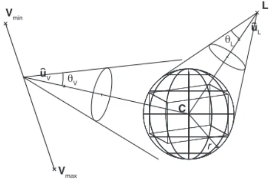
L Vmin Vmax uL uV C r θL θV ˆ ˆ
Figure 7: Based on the bounding sphere (C, r) of the current hierarchical level, we build bounding cones forbωV andbωL.
Both use the fact that the interval for V is restricted by the entry and exit points of the refracted camera ray, [Vmin, Vmax].
If a bounding volume hierarchy (BVH) is present in the renderer, we use it in a hierarchical descent: starting with the largest node containing the translucent object, we test whether it passes the first test. If yes, we iterate on its de-scendants. If not, we stop the search. We keep descending recursively until we reach triangles that have passed the first test. We apply to them the second test based on shading nor-mals.
If the renderer does not have a BVH, we test the triangles directly.
The output of the second test is both a boolean and a valid-ity interval for t. If the boolean is true, we apply Algorithm1
to this triangle.
For both tests, we build bounding cones forbωLand bωV (see Figure 7). We then use these cones to discard trian-gles where it is impossible to have a refracted path. We build these bounding cones using the the bounding sphere of the object (whether it is a triangle or a bounding volume), de-fined by its center C and radius r:
• bωLis inside a cone of axisbuLand angle θL: dLC = kL − Ck
buL = (L − C) /dLC θL = arcsin(r/dLC)
• bωV is bounded by a sweeping cone, whose normalized
axis moves frombuVmintobuVmaxand whose angle is θV:
buVmin = Vmin− C kVmin− Ck buVmax = Vmax− C kVmax− Ck θV = arcsin(r/dmin)
where dmin = min (kV − Ck) for V ∈ [Vmin, Vmax]
𝜂
𝜂
ˆ
ˆ
ˆ
ˆ
Figure 8: The half-vector bH lives inside a cone of axisbuH and angle θH.buH lives on an elliptical cone. This cone
in-tersects the plane perpendicular tobuNin an hyperbola. Ex-istence of a point such thatbuN+bH= 0 becomes a point-to-hyperbola distance in that plane.
Geometry-based test The spindle test tells us that the an-gle betweenbωV and bωL must be between
π
2 + arcsin(1/η)
and π. Alternatively, the angle betweenbωVand −bωLmust be smaller thanπ
2 − arcsin(1/η).
We compute the minimum angle between −buLandbuVand compare it withπ
2 − arcsin(1/η)+ θV+ θL. If it is larger, the
entire bounding sphere is outside of the spindle, and we can stop the search.
Shading-normal based test When testing against a trian-gle, we start by computing a sweeping cone bounding the half-vector bH. We also build a cone bounding the shading normal, with axisbuNand angle θNand check for intersection between the cones.
The tip of the normalized vectorbωLlies inside a sphere of radius rL = 2 sin(θL/2), centered on the tip ofbuL(similarly forbωV). Thus, the tip of H= ηbωV+bωLis inside a sphere of radius ηrV+ rL, centered on a moving vector ηbuV+buL.
We denote Hminthe minimal value of the norm of ηbuV+buL. The normalized half-vector bH lies inside a cone of axisbuH and angle θH:
buH = normalize(ηbuV+buL) θH = arcsin ((ηrV+ rL)/Hmin)
The axisbuH lies on a portion of an elliptic cone defined by buL and the circle on which ηbuV varies (see Figure8). It is possible to have bH+ NS = 0 only if −uH falls inside the
cone of axisbuNand angle θN+ θH.
Rather than having to compute the intersection of these two cones, we move to the plane perpendicular tobuN, de-fined by M ·buN = 1. The intersection between this plane and the cone (buN, θN+ θH) is a circle, of center O and radius tan(θN+ θH). The intersection between this plane and the
el-liptic cone carrying uH is a hyperbola. The two cones can
intersect only if the curves intersect in the plane: if the min-imum distance between O and the hyperbola is larger than tan(θN+ θH) we discard the triangle.
Restricting the interval for t A hyperbola defined as the intersection between a cone and a plane has two branches.
Only one branch is relevant for us, the one corresponding tobuN·buH < 0. The point V such thatbuN·buH = 0 defines the boundary between the two branches. We can discard the other part of the interval, which reduces the search interval for t.
3.2.5. Computing the integral
Once we have tminand tmaxfor a given triangle, we sample
this interval regularly in t. For K samples, we take: ti= tmin+
i+12
K (tmax− tmin) (18) For each tiwe compute Viusing Equation13, then Pion
the surface such that ViPiL is a valid path following Snell’s
law. We shoot a shadow ray from Pito L. If the points are
visible from each other, we add the contribution associated to that path, Ci, to the contribution of the triangle:
Ctriangle= tmax− tmin K X i Ci (19)
The number K of samples in each interval is a parameter. In practice, we have used K= 1 for all our test scenes with no visible impact on quality.
4. Results and comparison
Unless otherwise specified, pictures and timings in this pa-per were generated on a quad-core Intel Xeon W3250 at 2.66 GHz with 6 GB of memory, running Windows 7. We used the Mitsuba renderer [Jak10] for our algorithm, photon mapping and bi-directional path-tracing, and the original im-plementation of Walter et al.’s algorithm [WZHB09].
There is no post-processing in any of the pictures: no clamping, no filtering. We compute single scattering effects, along with transmitted and reflected light, as well as internal reflections.
4.1. Equal time comparison
The key advantage of our algorithm is that it provides high quality pictures of single scattering effects quickly. Figures1
and 9show a side-by-side comparison between our algo-rithm and other algoalgo-rithms for approximately the same com-putation time. Other algorithms do not provide the same quality:
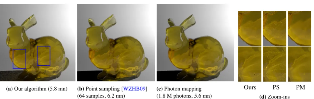
• Point sampling, the algorithm described in [WZHB09], computes an exact solution at several points along the re-fracted camera ray. With equal time computation, there are too little samples, and point artefacts are clearly visi-ble (see Figures1band9b).
• Photon mapping uses the implementation in the Mit-suba renderer, which relies on Beam-Radiance Esti-mates [JZJ08]. It provides a picture without artefacts, but the individual features characteristic of single scattering have been averaged (see Figures1cand9c).
PM, 150 M photons
Our algorithm Figure 10: Comparison with a high quality solution: Photon mapping with 150 M photons (3.53 h on a dual Intel Xeon E5345, 2.33 GHz with 48 Gb RAM).
• Bi-directional path-tracing also uses the implementa-tion in the Mitsuba renderer. For scattering effects, we connect paths from the light source and paths from the camera inside the medium. For single scattering, the two paths must intersect exactly, which has a zero probability for a point light source. To produce a picture, we replaced it with a spherical light source (see Figure 1d). Picture quality is much lower than for the other methods.
4.2. Validation: comparison with high-quality solution Given the difference between our results and those of other methods, we need confirmation that we are actually comput-ing the right solution. Photon mappcomput-ing with a large number of photons provides this validation. The computer we used in our tests ran out of memory after 15 million photons. We used a different computer, with 48 GB of memory, to com-pute a picture with 150 million photons (see Figure10). This high quality picture is identical to the one we compute in 169 s, up to the thinner details.
4.3. Equal-quality comparison
Increasing the number of samples or photons increases the quality of the other algorithms, along with their computation time. Figure11shows pictures with approximately the same quality. The computation time is at least 17 times larger, and the image quality is still not as good as ours. Note that bi-directional path tracing also converges to the same solution, but much slower than the other methods.
Equal quality comparisons with photon mapping is diffi-cult because of the memory cost: we are limited to 15 million photons on our testing computer. We allocated all of them to the volume photon map, specifically for single scattering. In a more realistic scenario, part of the photons would be used for surface effects and for multiple scattering, reducing the quality of single scattering simulation. On the other hand, photon mapping can be used for rendering more complex scenarios, that are beyond the scope of our method.
(a) Our algorithm (5.8 mn) (b) Point sampling [WZHB09] (64 samples, 6.2 mn) (c) Photon mapping (1.8 M photons, 5.6 mn) Ours PS PM (d) Zoom-ins
Figure 9: Comparison between our algorithm for single-scattering effects and existing methods, for approximately equal time. Bunny model with 16 301 triangles.
(a) Our algorithm (169 s) (b) Point sampling [WZHB09] (512 samples, 3 188 s, 18×)
(c) Photon mapping (15 M photons, 2 940 s, 17×)
(d) Bi-Directional Path-Tracing (500 K samples per pixel, 331 776 s, 1940×)
Figure 11: Comparison between our algorithm for single-scattering effects and existing methods, for approximately equal quality (Photon Mapping: we used the maximum number of photons for our computer, 15 millions; Bi-Directional Path-Tracing: we use a sphere instead of a point light source).
A strong advantage of our algorithm is that it has no addi-tional memory cost: we do not use any data structure beyond what is already present in the renderer: the geometry of the object and the bounding volume hierarchy.
4.4. Computation time
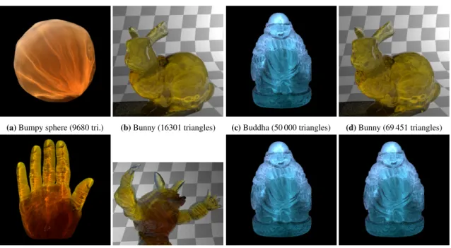
We used five test scenes, for a total of eight different poly-gon counts: the bumpy sphere from [WZHB09], the Stanford bunny at two different resolutions, a Buddha statue at three different resolutions, the Stanford armadillo and a model of a hand (see Figure12). Triangle count ranges from 104 to
106 triangles. For the Buddha and the hand, we show
com-putation times for two different light positions: from the top and from behind. We also tried different light positions for the bumpy sphere and the bunny, but the difference in com-putation time was within the margin of error.
Figure13adisplays the average computation time for each camera ray that reached the translucent object. This measure is independent of the screen coverage of the model. We show the computation time with and without shadow rays for each sample point. We show separately the average time for inter-nally reflected rays; 40 % to 55 % of the camera rays entering the object result in internal reflections (except for the bumpy sphere with only 20 %):
• The total computation time is dominated by finding the zeros of f. Shooting shadow rays accounts for 3 % of com-putation time. This could be caused, in part, by the sim-plicity of our test scenes: they contain a large translucent object and few other objects.
• The influence of light position depends on the object shape. For compact objects, such as the sphere, the bunny and the Buddha, it has little influence (at most 10 %).
(a) Bumpy sphere (9680 tri.) (b) Bunny (16301 triangles) (c) Buddha (50 000 triangles) (d) Bunny (69 451 triangles)
(e) Hand (310 000 triangles) (f) Armadillo (346 000 triangles) (g) Buddha (0.5 million tri.) (h) Buddha (1 million triangles) Figure 12: Our test scenes (by increasing order of complexity).
For branching objects, such as the hand and armadillo, it has a strong influence: computation time is several times smaller than for a compact object with the same trian-gle count if each branch can be treated independently (ar-madillo, hand illuminated from behind). It is slower than for a comparable compact object when branches interfere with each other (hand from the top).
• Scattering computations for internal reflections can be ei-ther slower or faster than for direct rays, depending on light position. The behavior evolves consistently with ob-ject resolution. Internal reflections are focusing compu-tations on part of the object, which can be more or less complex than the average.
Figure13bdisplays the same results in log-log space. For compact objects and identical lighting conditions, computa-tion time for each sample evolves roughly as O(n3/4), where
nis the number of polygons. A smooth curve drawn on a spherical object tesselated into n triangles crosses O(n1/2)
triangles. This is our lower bound. The upper bound is ex-ploring all triangles: O(n). Complexity is half-way between upper and lower bounds.
Comparing Figures 12b and 12d shows the effect of
changing object complexity: caustics become more convo-luted. The effect is less visible on the Buddha model (Fig-ures12c,12gand12h) probably because the first model is already of high accuracy.
5. Conclusion
We have described a new algorithm for accurate computa-tion of single scattering effects inside a translucent object with refractive boundary. It is an extension of Walter et al.’s algorithm [WZHB09]. Our main idea is to compute the lim-its of the influence of each triangle over each refracted ray, then sample only inside these limits. Our algorithm proves to be both faster and more accurate than existing methods, with a smaller memory footprint.
Our method does not require any additional memory structure beyond what is already available in a renderer: the geometry of each triangle, and a bounding volume hierar-chy. This makes it easier to implement inside existing ren-derers, but impacts performance: with adjacency informa-tion between triangles, we could reuse computainforma-tions from neighboring triangles for shared edges. This should reduce computation time by 50 %. Using the results from neighbor-ing pixels as a startneighbor-ing point for the Newton-Raphson iter-ation would also speed up computiter-ations. This informiter-ation would also help for adaptive anti-aliasing.
Our algorithm does not allow a speed-quality tradeoff. In future work we want to introduce this possibility, based on a hierarchical representation of surface details. This would also be connected to an extension to rough specular inter-face. We are currently limited to smooth dielectric.
Finally, we want to extend our algorithm to more complex configurations. There are no limitations on the camera ray, but we are restricted to one refractive interface between the
0 10 20 30 40 50 60 70 0 200000 500000 1e+06
Total computation time without auxiliary rays Internal reflections
Time per image sample (ms)
Number of triangles Hand
Armadillo
1st light position 2nd light position
(a) Linear representation
0.1 1 10 100
10000 100000 1e+06
Time per image sample (ms)
Number of triangles
Total computation time without auxiliary rays Internal reflections
O(n) O(n½) O(n¾)
Hand Armadillo
(b) Log-log space. Time per ray evolves approximately as n3/4.
Figure 13: Average computation time for each camera ray reaching the object, as a function of scene complexity, for two different light positions. Compact objects (bumpy sphere, bunny, Buddha) behave similarly (connected curves). For branching objects (hand, armadillo), complexity depends on light position.
camera ray segment and the light source. We would like to handle more complex cases, with several interfaces from the light source to the segment.
Acknowledgments
This work was supported in part by a grant ANR-11-BS02-006 “ALTA”. The Bunny and Armadillo models are provided by the Stanford Computer Graphics Lab data repository. The bumpy sphere model and the original [WZHB09] implementation were kindly pro-vided by Bruce Walter. The Agnes Hand model is propro-vided courtesy of INRIA by the AIM@SHAPE repository. The Buddha model is provided courtesy of VCG-ISTI by the AIM@SHAPE repository.
References
[EAMJ05] Ernst M., Akenine-M¨oller T., Jensen H. W.: Interac-tive rendering of caustics using interpolated warped volumes. In Graphics Interface(2005), pp. 87–96.2
[HDI∗10] Hu W., Dong Z., Ihrke I., Grosch T., Yuan G., Sei-del H.-P.: Interactive volume caustics in single-scattering media. In Symposium on Interactive 3D Graphics and Games (2010), ACM, pp. 109–117.2
[IDN01] Iwasaki K., Dobashi Y., Nishita T.: Efficient rendering of optical effects within water using graphics hardware. In Pa-cific Conference on Computer Graphics and Applications(2001), pp. 374–383.2
[Ige99] Igehy H.: Tracing ray differentials. In SIGGRAPH ’99 (1999), ACM, pp. 179–186.3
[IZT∗07]
Ihrke I., Ziegler G., Tevs A., Theobalt C., Magnor M., Seidel H.-P.: Eikonal rendering: Efficient light transport in refrac-tive objects. ACM Transactions on Graphics (proc. Siggraph) 26, 3 (July 2007), 59:1 – 59:9.2
[Jak10] Jakob W.: Mitsuba renderer, 2010. http://www. mitsuba-renderer.org.8
[JNSJ11] Jarosz W., Nowrouzezahrai D., Sadeghi I., Jensen H. W.: A comprehensive theory of volumetric radiance esti-mation using photon points and beams. ACM Transactions on Graphics 30, 1 (January 2011), 5:1–5:19.2
[JNT∗11]
Jarosz W., Nowrouzezahrai D., Thomas R., Sloan P.-P., Zwicker M.: Progressive photon beams. ACM Transactions on Graphics (proc. Siggraph Asia) 30, 6 (December 2011), 181:1– 181:12.2
[JZJ08] Jarosz W., Zwicker M., Jensen H. W.: The beam radiance estimate for volumetric photon mapping. Computer Graphics Forum (Proc. Eurographics 2008) 27, 2 (2008), 557 – 566.2,8
[NN94] Nishita T., Nakamae E.: Method of displaying optical effects within water using accumulation buffer. In SIGGRAPH ’94(1994), ACM, pp. 373–379.2
[PP09] Pegoraro V., Parker S. G.: An Analytical Solution to Sin-gle Scattering in Homogeneous Participating Media. Computer Graphics Forum (Proc. Eurographics 2009) 28, 2 (2009), 329– 335.2
[Ree11] Reeder M.: The kernel of a three-by-three matrix.
https://www2.bc.edu/~reederma/Linalg15.pdf, 2011.6
[SZLG10] Sun X., Zhou K., Lin S., Guo B.: Line space gather-ing for sgather-ingle scattergather-ing in large scenes. ACM Transactions on Graphics (proc. Siggraph 2010) 29, 4 (July 2010), 54:1–54:8.2
[SZS∗08]
Sun X., Zhou K., Stollnitz E., Shi J., Guo B.: Interac-tive relighting of dynamic refracInterac-tive objects. ACM Transactions on Graphics (proc. Siggraph 2008) 27, 3 (Aug. 2008), 35:1–35:9.
2
[WZHB09] Walter B., Zhao S., Holzschuch N., Bala K.: Sin-gle scattering in refractive media with trianSin-gle mesh boundaries. ACM Transactions on Graphics (proc. Siggraph 2009) 28, 3 (July 2009), 92:1–92:8.1,2,3,4,8,9,10,11
Appendix A: Complexity of the equation f= 0
f = 0 defines a polynomial equation of degree at most 6 in the parameters t, a and b.
Proof
Each vector V, P and Ns (before normalization) can be
ex-pressed linearly with a parameter vector x= (t, a, b, 1)|:
V = Vmin+ t
Vmax− Vmin
kVmax− Vmink
= MVx (20)
Ns = N0+ a(N1− N0)+ b(N2− N0)= MNx (22)
Vectors L − P and V − P are also linear:
L − P = L − MPx= MLPx (23)
V − P = MVx − MPx= MV Px (24)
Solutions for f= 0 must satisfy Snell’s law:
η sin θi= sin θo (25)
We express this law with our variables using cross products: ηk(V − P) × Nsk
kV − PkkNsk
=k(L − P) × Nsk
kL − PkkNsk
(26) All points solutions of the equation f= 0 satisfy:
η2(L − P)2k(V − P) × N
sk2= (V − P)2k(L − P) × Nsk2 (27)
(L − P)2 and (V − P)2 are polynomials of degree 2. Each
coordinate of (V−P)×Nsand (L−P)×Nsis a polynomial of
degree 2. The square of their norm is a polynomial of degree 4. Thus, Equation27is a polynomial equation of degree 6.