Compiling Elementary Mathematical Functions into Finite Chemical Reaction Networks via a Polynomialization Algorithm for ODEs

HAL Id: hal-03220725

https://hal.inria.fr/hal-03220725v2

Submitted on 27 Jun 2021

HAL is a multi-disciplinary open access

archive for the deposit and dissemination of

sci-entific research documents, whether they are

pub-lished or not. The documents may come from

L’archive ouverte pluridisciplinaire HAL, est

destinée au dépôt et à la diffusion de documents

scientifiques de niveau recherche, publiés ou non,

émanant des établissements d’enseignement et de

Compiling Elementary Mathematical Functions into

Finite Chemical Reaction Networks via a

Polynomialization Algorithm for ODEs

Mathieu Hemery, François Fages, Sylvain Soliman

To cite this version:

Mathieu Hemery, François Fages, Sylvain Soliman. Compiling Elementary Mathematical Functions

into Finite Chemical Reaction Networks via a Polynomialization Algorithm for ODEs. Proceedings

of the nineteenth international conference on Computational Methods in Systems Biology„ Sep 2021,

Bordeaux, France. �hal-03220725v2�

Compiling Elementary Mathematical Functions

into Finite Chemical Reaction Networks

via a Polynomialization Algorithm for ODEs

Mathieu Hemery, François Fages, and Sylvain Soliman

Inria Saclay Île-de-France, EPI Lifeware, Palaiseau, France

Abstract. The Turing completeness result for continuous chemical re-action networks (CRN) shows that any computable function over the real numbers can be computed by a CRN over a finite set of formal molecular species using at most bimolecular reactions with mass action law kinet-ics. The proof uses a previous result of Turing completeness for functions defined by polynomial ordinary differential equations (PODE), the dual-rail encoding of real variables by the difference of concentration between two molecular species, and a back-end quadratization transformation to restrict to elementary reactions with at most two reactants. In this paper, we present a polynomialization algorithm of quadratic time complexity to transform a system of elementary differential equations in PODE. This algorithm is used as a front-end transformation to compile any ele-mentary mathematical function, either of time or of some input species, into a finite CRN. We illustrate the performance of our compiler on a benchmark of elementary functions relevant to CRN design problems in synthetic biology specified by mathematical functions. In particular, the abstract CRN obtained by compilation of the Hill function of order 5 is compared to the natural CRN structure of MAPK signalling networks.

1

Introduction

Chemical reaction networks (CRN) provide a standard formalism in chemistry and biology to describe, analyze, and also design complex molecular interaction networks. In the perspective of systems biology, they are a central tool to an-alyze the high-level functions of the cell in terms of their low-level molecular interactions. In the perspective of synthetic biology, they constitute a target programming language to implement in chemistry new functions in either living cells or artificial devices.

A CRN can be interpreted in a hierarchy of Boolean, discrete, stochastic and differential semantics [7,13] which is at the basis of a rich theory for the analysis of their dynamical properties [14,9,1], and more recently, of their computational power [7,6,11]. In particular, their interpretation by Ordinary Differential Equa-tions (ODE) allows us to give a precise mathematical meaning to the notion of analog computation and high-level functions computed by cells [10,25,23], with the following definitions:

Definition 1. [11,16,26] A function f : R+ → R+ is generated by a CRN

on some species y with given initial concentrations for all species, if the ODE associated to the CRN has a unique solution verifying ∀t ≥ 0 y(t) = f (t).

That first definition states that a positive real function of one positive argu-ment is generated by a CRN for some given initial concentration values, if the graph of that function is given by the temporal evolution of the concentration of one molecular species in that CRN.

Definition 2. [11,16]1 _{A function f : R}+ → R+ is computed by a CRN for

some input species x, output species y, and initial concentrations given for all species apart from x, if for any input concentration value x(0) for x, the ODE initial value problem associated to the CRN has a unique solution satisfying limt→∞y(t) = f (x(0)).

The second definition states that the same function is computed by a CRN if for any input x ≥ 0, and initialization of the CRN input species to value x, the CRN output species converges to the result f (x). That definition for input/output functions computed by a CRN is used in [11] to show the Turing completeness of continuous CRNs in the sense that any computable function over the real numbers can be computed by a CRN over a finite set of formal molecular species using at most bimolecular reactions with mass action law kinetics. The proof uses a previous result of Turing completeness for functions defined by polynomial ordinary differential equation initial value problems (PIVP) [2], the dual-rail encoding of real variables by the difference of concentration between two molecular species [21,18], and a back-end quadratization transformation to restrict to elementary reactions with at most two reactants [5,19,3]. This proof gives rise to a pipeline, implemented in BIOCHAM-42, to compile any computable real function presented by a PIVP into a finite CRN.

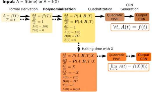
However in practice, it is not immediate to define a PIVP that generates or computes a desired function. In this article, we solve this problem for elemen-tary functions over the reals, by adding to our compilation pipeline a front-end module to transform any elementary function in a PIVP which either generates or computes that function, as schemtized in Fig. 1.

More precisely, we present a polynomialization algorithm to transform any Elementary ODE system (EODE), i.e. ODE system made of elementary dif-ferential functions, into a polynomial one (PODE). This algorithm proceeds by introducing variables for computing the non-polynomial terms of the input, eliminating such terms from the ODE by rewriting, and obtaining the ODE for the new variables by formal derivation. The derivation steps may bring new non-polynomial terms requiring new variables. We show the termination of that

1 _{For the sake of simplicity of the definition given here, we omit the error control}

mechanism that requires one extra CRN species z verifying: ∀t > 1 |y(t) − f (x(0))| ≤ z(t), ∀t0

> t z(t0) < z(t) and limt→∞z(t) = 0. 2

http://lifeware.inria.fr/biocham/. All experiments described in this paper are available at https://lifeware.inria.fr/wiki/Main/Software#CMSB21

Fig. 1. Polynomialization step in the complete pipeline for compiling a formally differ-entiable function f (termination is proved here for elementary functions) into a finite CRN, either a function of time (plain arrows) or an input/output function (dashed arrows): P and P are polynomials, and B denotes the set of species introduced by polynomialization given with initial conditions IC.

algorithm, with quadratic time complexity, and that only a linear number of new variables, in terms of the size of the input expression, are actually needed.

Related work includes one method described in [24] to compute some polyno-mial abstractions of a non-polynopolyno-mial system. That method progresses top-down from some set of possible functions given a priori, and progressively sieves them down to a polynomial system. This permits to choose the degree of the poly-nomial abstraction, but that method may fail if the starting set of functions, or the chosen degree, are too small. On the other hand, our algorithm proceeds bottom-up, by introducing the functions when needed, with no choice a priori. A bottom-up approach closer to ours is also mentioned in [17] but for a very restricted grammar of functions while we develop here a general algorithm and prove its termination on the whole class of elementary mathematical functions. The rest of the paper is organized as follows. In the next section, we describe the language of elementary function that are accepted as input of our compila-tion pipeline into CRN. In Sec. 3, we present a general polynomializacompila-tion algo-rithm for elementary ODEs, prove its termination, and show its quadratic time complexity. In Sec. 4 we describe the use of this algorithm as a front-end trans-formation in our compilation pipeline to compile any elementary mathematical function into a finite CRN. In Sec. 5 we evaluate this approach on a benchmark of elementary functions relevant to CRN design problems in synthetic biology

used in [19]. In particular, we compare the CRN synthesized for the Hill function of order 5 to the structure of the natural MAPK signalling CRNs that have been shown to implement a similar input/output function [20]. Finally, we conclude on the results achieved and several perspectives for future work.

2

Input Language of Elementary Functions

Let us consider the problem of synthesizing a CRN to generate the function of time: A(t) = log(1+t2_{) in the sense of Def. 1. The compilation method described}

in [11] takes as input a PIVP which admits that function as solution on variable A. Here, we want to automate the construction of such a PIVP.

The first step of our front-end transformation schematized in Fig. 1, is to determine an ODE which admits that function of time as solution. For this, one can simply take the derivative of the equation with respect to time and set as initial condition the value for the desired function at 0, giving:

dA dt =

2t

1 + t2 A(0) = 1

Then we need to transform this ODE into a PODE. Our polynomialization algorithm will introduce a new variable B = _1+t12, and similarly compute its

derivative and its initial value, as follows: dB

dt = −2t

(1 + t2₎2 = −2tB

2 _{B(0) = 1}

We also need to introduce a variable T for time with dT_dt = 1 and T (0) = 0. giving the following PIVP:

dA dt = 2.T.B dB dt = −2.T.B 2 dT dt = 1 A(0) = 1 B(0) = 1 T (0) = 0

Note that the termination of those transformations is not obvious in general. It is proved in the next section. That PIVP of degree 3 can now be used as input of our previous compilation pipeline [11]. It is first transformed in quadratic form [19], in this case by introducing one variable, BT = B.T , and removing the time T , giving the following quadratic PIVP:

dA dt = 2.BT dB dt = −2.BT.B d(BT ) dt = dB dt.T + B dT t = −2.BT 2_{+ B} A(0) = 1 B(0) = 1 BT (0) = 0

One reaction with mass action law kinetics is then generated for each mono-mial of the ODE. Since in this example the reactions are well-formed and strict

the system is positive (lemma 1 in [12]). There is thus no need to introduce dual-rail variables for negative values, and the generated elementary CRN (with rate constants written above the arrow) is:

B + BT −→ BT2 B −→ B + BT1

2.BT −→ BT2 BT −→ A + BT2 B(0) = 1

Now, it is worth noting that if we want to synthesize a CRN that computes (instead of generating) the function log(1 + x2) of some input x in the sense of Def. 2, the general method described in [22,11] consists in introducing a variable X, initialized to value x, multiplying the terms of the PIVP for generating the function, and following a decreasing exponential to halt the PIVP on the prescribed input. The previous PIVP of degree 3 thus becomes a PIVP of degree 4 by this transformation: dX dt = −X dA dt = 2.T.B.X dB dt = −2.T.B 2_.X dT dt = X X(0) = x A(0) = 1 B(0) = 1 T (0) = 0 The quadratization algorithm [19] now introduces new variables BX and T BX for the corresponding monomials, and removes variables T and B. This generates the following quadratic PIVP:

dX dt = −X dBX dt = dB dt X + B dX dt = −2.BX.T BX − BX dA dt = 2.T BX dT BX dt = BX.X − 2.T BX 2_{− T BX} X(0) = x BX(0) = x A(0) = 1 T BX(0) = 0

and finally the following elementary CRN which computes the log(1 + x2) func-tion:

BX + TBX −→ TBX2 X −→ ∅1 BX −→ ∅1 BX + X−→ BX + TBX + X1 TBX −→ ∅1

2.TBX −→ TBX2 TBX −→ A + TBX2

X(0) = x BX (0) = x A(0) = 1

2.2 Elementary Functions as Compilation Pipeline Input Language In mathematics, elementary functions refer to unary functions (over the reals in our case) that are defined as a sum, product or composition of finitely many polynomial, rational, trigonometric, hyperbolic, exponential functions and their inverses. Most of these functions are defined on the real axis but a few exceptions are worth mentioning: the inverse of some function is restricted to the image of

R by the function (e.g., arccos is only defined on [−1, 1]) and the exponentiation may be non-analytic in 0 and is thus considered elementary only on an open interval that does not include 0.

The set of elementary functions of x is formally defined as the least set of functions containing:

– Constants: 2, π, e, etc.

– Polynomials of x : x + 1, x2_{, x}3_{− 42.x, etc.}

– Powers of x :√x, √3_{x, x}−4_{, etc.}

– Exponential and logarithm functions: ex, ln x – Trigonometric functions: sin x, cos x, tan x, etc. – Inverse trigonometric functions: arcsin x, arccos x, etc. – Hyperbolic functions: sinh x, cosh x, etc.

– Inverse hyperbolic functions: arsinh x, arcosh x, etc.

and closed by arithmetic operations (addition, subtraction, multiplication, divi-sion) and composition. Elementary functions are also closed by differentiation but not necessarily by integration. On the other hand hyper-geometric func-tions, Bessel funcfunc-tions, gamma, zeta funcfunc-tions, are examples of (computable) non-elementary functions.

3

Polynomialization Algorithm for Elementary ODEs

The core of Alg. 1 for polynomializing an EODE system is the detection of the elements of the derivatives that are not polynomial and their introduction as new variables. Then symbolic derivation and syntactic substitution allow us to compute the derivatives of the new variables and to modify the system of equations accordingly.

It is worth noting that the list of substitutions has to be memorized along the way, therefore handling an algebraic-differential system during the execution of the algorithm, since they may reappear during the derivation step. This typically occurs when the derivation graph harbors a cycle like: cos → sin → cos (Fig. 2). Nevertheless, a particular treatment has to be applied to the case of non-integer or negative power as they form an infinite set and may thus produce infinite chains of derivations. This can be seen if we try to apply naively Alg. 1 on this simple example:

dA dt = A

0.4

for which we introduce the new variable B = A0.4 _with

dB

dt = 0.4A

−0.6 dA

dt = 0.4A

−0.2

At this point, it is tempting to introduce C = A−0.2 but that would lead to an infinite loop, introducing more and more powers of A.

Algorithm 1 Polynomialization of an EODE system

1: Input: A set of ODEs of the form {x0= fx(x, y, . . .), y0= fy(x, y . . .), . . .}.

2: Output: A set of PODEs where the initial variables x, y, . . . are still present and accept the same solutions.

3: Initialize T ransf ormations ← ∅ and P olyODE ← ∅ 4: while ODE is not empty do

5: take and remove V ar0= Derivative from ODE;

6: N ewDerivative ← apply T ransf ormations to Derivative;

7: T erms ← set of maximal non-polynomial subterms of N ewDerivative; 8: for all T erm in T erms do

9: add (T erm 7→ N ewV ar) to T ransf ormations; 10: T ermDerivative ← the symbolic derivative of T erm; 11: add (N ewV ar0= T ermDerivative) to ODE;

12: P olyDerivative ← apply T ransf ormations to Derivatives; 13: add (V ar0= P olyDerivative) to P olyODE;

14: return P olyODE

This can be easily avoided by introducing C = _A1 instead, then: dB dt = 0.4B 2_C dC dt = − 1 A2 dA dt = −C 2_B

There is therefore a specific treatment to do when introducing the new variable of an exponentiation in order to force the algorithm to use the inverse variable instead of an infinite sequence of variables. For this, when adding the new vari-able N = Xp to the system, we explicitly replace the expression Xp−1 by N/X in the derivatives, thus making the use of 1/X a natural consequence. Of course, this makes the final PODE non analytic in X = 0. This is linked to the fact that exponentiation apart from the polynomial case is actually not analytic in 0, and it is thus not surprising that computation fails if we reach a time where X = 0.

3.2 Interval of definition

Elementary functions are analytic upon open interval of their domain, but may suffer from non-analyticity on the boundary. For example exponentiation with a non integer coefficient may be extended by continuity in 0 but is not analytic here. During our polynomialization, this kind of behaviour may lead to the ap-pearance of species that diverge on these points. This is important as it can be shown that only analytic functions can be generated by a PIVP.

In particular, the absolute value function over the reals is elementary as it can be expressed as the composition of a power and root of x : |x| =√x2_{. But is not}

analytic on 0. Hence, if we consider the EODE dx_dt = |x|, our polynomialization will introduce the variables y = |x| and z = _x1, to obtain the PODE:

dx dt = y dy dt = y 2_.z dz dt = −(z 2_.y)

And when x approaches 0, the variable z, its inverse, will diverge.

The unicity of the solution of a PIVP is constrained by the initial conditions, but this unicity is not ensured when passing a non-analyticity. A consequence of this remark is that our compiled solution is defined from its initial condition (t = 0) up to the first non-analyticity of the compiled function.

3.3 Termination

Before proving the termination of our algorithm for the input set of elementary functions over the reals, we can show a general lemma for any set F of formally differentiable, possibly multivariate, real functions. Let F denote the closure of F ∪ R by addition and multiplicationi, that is the algebra of F over R.

Lemma 1. For any finite set F of formally differentiable functions over the reals such that ∀f ∈ F, f0 ∈ F , Alg. 1 terminates.

Proof. In the while loop, since we detect all the non-polynomial parts of the derivatives in one pass, we are sure that the derivative at hand in each while step becomes polynomial. New variables may however be introduced in such a step, thus the only possibility of non-termination is to introduce an infinity of new variables.

The proof of termination proceeds by cases on the structure of the derivatives. Suppose we have an ODE on the set of variables {Xi} with i ∈ [1, n] and let

us denote by d(Xi) the derivative of Xi. First, it is obvious that if d(Xi) is a

single variable or a constant (numeric or parameter) then we have nothing to do. Similarly, for every expression composed by addition or multiplication of such terms, they are already polynomial.

If the new variable is a function of several variables (here 2): Y = f (Xj, Xk),

we have: dY dt = ∂f (Xj, Xk) ∂Xj d(Xj) + ∂f (Xj, Xk) ∂Xk d(Xk)

and as the addition is allowed in polynomial, we can consider separately the two derivatives. Thus, we can restrict ourselves to the case of functions of a single variable.

For a function of a single variable with no composition we have: dy dt = df (Xi) dt = f 0_(X i)d(Xi)

we have seen that d(Xi) is already polynomial but nothing ensures that f0 is.

However by definition of our set F , f0_(X

i) may be expressed with other

func-tion of X in the set F , all applied to Xi, since composition is not allowed in

the construction of F . As the set F is finite, we are sure to terminate after in-troducing at most |F | variables. It is thus important to not include the closure by composition in the definition of our set F . Indeed a function such that its derivative would be of the form: f0(x) = f (f (x)) may lead to an infinite loop for our algorithm.

Finally, when facing a composition, e.g. f (g(X)), we replace it by a new variable, say y, with the standard derivation rule:

dy dt = df (g(Xi)) dt = f 0_(g(X i))g0(Xi)d(Xi)

We thus have two different chains of variables to introduce: at first f (g(x)), f0(g(x)), f00(g(x)), etc. and in a second time: g0(x), g00(x). The important point to remark is that there is no mixing: all derivatives of f are applied to g(x) and neither to the derivatives of g. By the same argument as for the case without composition, the polynomialization of both f0(g(Xi)) and g0(Xi) terminates.

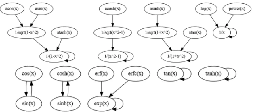
Fig. 2. Dependency graph of the derivatives for the elementary functions. Each function is given up to a polynomial composition, hence the derivative of arccos x which is_√1

1−x2

points to the √1

x node. Note that the out-degree of each node is 1 as the derivative of

each of these functions is always a single function or the composition of a polynomial and a single function.

Corollary 1. Alg. 1 terminates on elementary functions.

Proof. Let F be the set of elementary functions. Fig. 2 displays the dependency graph of the set F and its derivatives. Apart from the exponentiation, we can see that this set obeys to the condition of Lemma 1.

The only difficulty thus comes from the exponentiation as it actually defines an infinite set of functions of the form f (x) = xα _{for any real constant α.}

Nevertheless, as explained above, the algorithm terminates also in this case since we express the derivative in the form:

f0(x) = αxα−1= αf (x)1

x (1)

and the inverse function is in F , henceforth the case of exponentation also ter-minates.

3.4 Complexity

To estimate the computational time complexity of Alg. 1, let us first determine a bound on the number of new variables introduced in the system.

Proposition 1. Alg. 1 introduces at most a linear number of variables in the size of the input.

Proof. For each elementary function f , represented in Fig. 2, we have to intro-duce recursively all the functions on which rely its derivative, in terms of the (directed) dependency graph, this is the reachable set starting from f . In this case the largest reachable set is of cardinal 3. More generally, let us call ` the cardinal of the largest set of reachable nodes starting form a single node. Then, each elementary function that is not already polynomial introduces at most ` variables.

Hence, we have to introduce at most `F variables where F is the number of functions used in the ODE. Of course, F is bounded by the size of the input. Proposition 2. Alg. 1 has a quadratic time complexity.

Proof. To introduce a new variable, we have to first compute its derivative, and then substitute its expression in the reminder of the ODE. Both operations are linear in the size of the current system size, and we just have seen that this one will grow at most as a linear function of the input size, giving only a linear dependency. Thus, our algorithm is quadratic in the size of the input.

3.5 Remark on the Compilation of the Exponentiation

In the compilation of the exponentiation described in Sec. 3.1 we introduce two variables, but this raises an interesting question concerning the conditions under which a differential equation of the form: dA

dt = A

α

can be set in polynomial form by introducing only one variable. Indeed, if we introduce B = Aβ _{we have:}

dB dt = βA

β−1 dA

dt = βA

α+β−1

and to be polynomial we need to find four positive integers i, j, k, l such that:

α = i + jβ α + β − 1 = k + lβ

We thus need that α be of the form: α = j(k + 1) + i(1 − l) j + 1 − l

Clearly, only a fractional power can be reduced in one step. Now suppose that α = p_q then we have by identifying numerator and denominator and setting l = 2:

j = q − 1 + l = q + 1 and k = p + i 1 + q − 1

an equation that always admits solutions with i and k positive. For example α = 1₃ may be solved with β = −2₃ and i = 3, j = 4, k = 0, l = 2. But this uses a polynomial of order 7 which may impact negatively the final quadratization phase [19]. For these reasons, we chose to treat exponentiation by systematically introducing two variables.

4

CRN Compilation Pipeline for Elementary Functions

To illustrate the behavior of our complete pipeline schematized in Fig. 1, let us consider the compilation of the Hill function H = _1+xx into a CRN that computes H(x) in the sense of Def. 2, i.e., such that the final concentration of species H gives the result limt→∞H(t) = _1+xx .

The first step of the front-end transformation is to introduce a pseudo-time variable: T = t and replace the input X by T in the expression H = _1+TT , and then to compute the formal derivative of H to obtain the ODE:

dH dt = 1 (1 + T )2 dT dt = 1

The second step is to polynomialize that ODE with Alg. 1. This is done by examining the right hand side of the derivative of H and introduce as new variable A = _{(1+T )}1 which allows us to rewritedH_dt = A2_{. We also need to compute}

the derivative of this new variable: dA

dt = −A

2_{, A(0) = 1}

This PIVP generates the time function H(t) in the sense of Def. 1.

Now, we enter the compilation pipeline from PIVP described in [11]. To compute the function H(x) of input x, a new variable X that obeys a decreasing exponential is introduced and used to halt all other derivatives at time x:

dH dt = A 2_.X dX dt = −X dA dt = −A 2_.X dT dt = X H(0) = 0 X(0) = x A(0) = 1 T (0) = 0

Then the quadratization step [19], introduces the new variable B = A.X. Inter-estingly, intermediary variables X and T are no longer used and removed. We finally get: dH dt = A.B dB dt = −B − B 2 dA dt = −A.B H(0) = 0 B(0) = x A(0) = 1

And the compiled CRN is:

B −→ ∅1 A + B−→ B + H1 2.B−→ B1 A(0) = 1 B(0) = input

4.2 Implementation

Alg. 1 is implemented by rewriting formal expressions using a simple algebraic normal form and standard derivation rules.

The most computationally expensive step of our complete compilation pipeline in Fig. 1 is the quadratization of the intermediate PIVP to a PIVP of order at most 2. This step is necessary to restrict ourselves to elementary reactions with at most two reactants which are more amenable to real implementations with real enzymes. While the existence of a quadratic form for any PODE can be sim-ply shown by introducing an exponential number of variables [5], the problem of minimizing the dimension of that quadratization is NP-hard [19]. In the im-plementaiton of BIOCHAM used in the next section, we use both the MAXSAT algorithm described in [19] (option sat_species below) and a heuristic algo-rithm (option fastnSAT below) to first obtain a subset of variables guaranteed to contain a quadratic solution, and then call the MAXSAT solver (RC23_{) to}

minimize the dimension in that quadratization.

5

Evaluation

In this section, we consider the benchmark of functions already considered in [19] for quadratization problems. Table 1 gives some performance figures about the complete compilation pipeline in terms of total computation time and size of the synthesized CRNs, with the two options discussed above for quadratization. It is worth noting that those synthetic CRNs are not unique and that other CRNs could be synthesized for the same function, by making different choices in both our polynomialization and quadratization algorithms. Even when imposing optimality in the number of introduced variables, there may exist several optimal CRNs. For example, the two CRNs obtained for Hill4 compiled with the two options for quadratization are different but both have the same number of species and reactions (Table 1).

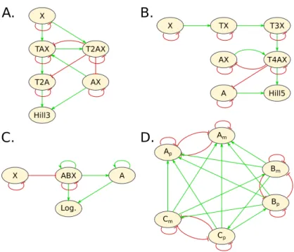
Let us examine the influence graphs of those synthetic CRNs since they provide a more compact abstract representation of the reaction graph [13]. Fig. 3 depicts the influence graphs between molecular species of the synthesized CRNs for the hill functions of order 3 (Fig. 3A.) and 5 (Fig. 3B.), the logistic function (Fig. 3C) and the square of the cosine function (Fig. 3). One can remark on those examples that the outputs of the synthesized CRN do not participate in any feedback reaction. This is however not necessarily the case of the CRNs synthesized by our pipeline, as shown for instance by the cosine function [11]. More precisely, the Hill3 CRN in Table 1 synthesized with the sat_species

3

fastnSAT sat_species Function time number of number of time number of number of

(ms) species reactions (ms) species reactions Hill1 80 4 5 85 3 3 Hill2 90 6 10 82 5 8 Hill3 100 6 10 115 6 12 Hill4 100 7 13 162 7 13 Hill5 110 8 16 550 7 11 Hill10 160 13 31 timeout Hill20 380 23 61 timeout Logistic 80 3 5 85 3 5 Double exp. 80 3 4 85 3 4 Gaussian 85 3 4 85 3 4 Logit 95 4 7 100 4 6

Table 1. Performance results on the benchmark of CRN design problems of [19] in terms of total compilation time, and size of the synthesized CRN with two options for quadratization.

option is the following:

x −→ ∅1 Ax −→ ∅1 TAx −→ ∅1 T2Ax −→ ∅1

Ax + T2Ax −→ T2Ax3 Ax + x −→ Ax + TAx + x1 T2Ax + TAx −→ T2Ax3 TAx−→ T2A + TAx2 T2A + T2Ax −→ T2Ax3 TAx + x−→ T2Ax + TAx + x2

2.T2Ax −→ T2Ax3 Ax + T2A−→ Ax + T2A + hill32 x (0) = input Ax (0) = input

The Hill5 CRN in the table synthesized with the same option is: x −→ ∅1 Ax −→ ∅1

Tx −→ ∅1 T3x −→ ∅1

T4Ax −→ ∅1 A + T4Ax −→ T4Ax + hill55 Ax + T4Ax −→ T4Ax5 2.x −→ Tx + 2.x1

2.Tx −→ T3x + 2.Tx3 Ax + T3x −→ Ax + T3x + T4Ax4 2.T4Ax −→ T4Ax5 x(0) = input

A(0) = 1 Ax (0) = input

From our computational point of view, the Hill5 CRN above is one syn-thetic analog of the natural MAPK CRN among others. Indeed, the natural

Fig. 3. Influence graphs of four of the synthetic CRNs of Table 1. A. and B. respec-tively implement the Hill function of order 3 and 5. C. corresponds to the logistic function and D. computes the square of the cosine of the time. In this last example, the output is only read on Apbut the presence of its negative part Am is actually a

crucial part of the computation despite having an essentially null concentration.

MAPK signalling network has been shown in [20] to compute an ultrasensitive input/output function which is well approximated by a Hill function of order 4.9. Both the natural MAPK CRN and the synthetic Hill5 CRN thus compute a sim-ilar input/ouput function and it makes sense to try to compare their structure. In term of size, the MAPK model of [20] comprises 22 species and 30 reactions, while the Hill5 CRN synthesized by our pipeline now uses only 7 formal molec-ular species and 11 elementary reactions. This shows a huge improvement with respect to our first results reported in [11] where several tens of reactions were synthesized for Hill functions. In term of topological structure, we have checked that there exists (several) subgraph epimorphisms [15] mapping the MAPK CRN to that Hill5 CRN, meaning that the MAPK CRN somehow contains the core structure of the synthetic Hill5 CRN in some non-trivial sense. The biological significance of those relationships is however still unclear, although one could expect to explain it in terms of robustness properties [4]. It is also worth noting that in the natural MAPK CRN structure, the input is a catalyst that is not consumed by the downward reactions, whereas in our CRN synthesis scheme, the input is generally consumed by the downward reactions. The MAPK

net-work thus illustrates a case of online analog computation which is currently not treated by our theoretical framework.

6

Conclusion and Perspectives

We have presented an algorithm to transform any system of elementary ordinary differential equations in a polynomial ordinary differential equation system pre-serving the solutions of the original variables. This algorithm of quadratic time complexity introduces at most a linear number of new variables. This algorithm allows us to automatically compile any elementary mathematical function into a finite CRN, using a pipeline of transformations starting from the formal deriva-tion of the elementary funcderiva-tion to generate or compute, the polynomializaderiva-tion of the elementary ODE, and continuing with the previous pipeline of [11] for the dual-rail encoding of negative values of the PODE [18,21], the quadratization of the PODE [19], and the synthesis of elementary reactions for the quadratic ODEs [12].

The implementation in BIOCHAM-4 of this complete pipeline has been used to illustrate the CRNs synthesized for a variety of elementary mathematical functions used as specification. In particular, the CRN synthesized for the Hill function of order 5 provides a synthetic analog of the MAPK signalling net-work which has been shown to compute a similar ultrasensitive input/output function [20]. In this compilation process, the quadratization part is the most complex one since minimizing the dimension of the result is a NP-hard prob-lem [19]. On the benchmark presented here, our maxSAT impprob-lementation is sufficient but we also use by default a heuristic algorithm that trades optimality for better performance. It should also be noted that a new algorithm has been recently proposed for the global optimization problem in [3].

This work may be improved in several directions. We might extend this ap-proach to multivariate functions. This is not trivial as the trick of halting the time at the input value needs be generalized to several inputs.

Another important point is to investigate is the variety of different CRNs that can be synthesized by our pipeline. As pointed out earlier, there may be several optimal solutions to the quadratization problem and there may similarly be several polynomializations of a given ODE introducing the same number of variables. Our pipeline make choices to deterministically propose one solution, but being able to explore the set of solutions and compare their properties with respect to metrics like robustness to initial conditions or reaction rates, or im-posing some similarity requirement with a given biological solution would be interesting.

Furthermore, the comparison to the MAPK network also points to the inter-esting class of online computation which does not consume the inputs, whereas in our approach the input species are consumed, and the synthesized CRN would need to be reinitialized for another computation. This limitation is not a problem for one-shot CRN programs such as those designed for medical diagnosis

applica-tions [8], but synthesizing a CRN for computing an input/output function online appears to be a harder problem worthy of further theoretical investigation.

Acknowledgment We acknowledge fruitful discussions with Olivier Bournez, Gleb Pogudin and Amaury Pouly. This work was supported by ANR-DFG SYM-BIONT “Symbolic Methods for Biological Networks” project grant ANR-17-CE40-0036, and ANR DIFFERENCE “Complexity theory with discrete ODEs” project grant ANR-20-CE48-0002.

References

1. Adrien Baudier, François Fages, and Sylvain Soliman. Graphical requirements for multistationarity in reaction networks and their verification in biomodels. Journal of Theoretical Biology, 459:79–89, December 2018.

2. Olivier Bournez, Manuel L. Campagnolo, Daniel S. Graça, and Emmanuel Hainry. Polynomial differential equations compute all real computable functions on com-putable compact intervals. Journal of Complexity, 23(3):317–335, 2007.

3. Andrey Bychkov and Gleb Pogudin. Optimal monomial quadratization for ode systems. In Proceedings of the IWOCA 2021 - 32nd International Workshop on Combinatorial Algorithms, July 2021.

4. Luca Cardelli. Morphisms of reaction networks that couple structure to function. BMC systems biology, 8(84), 2014.

5. David C. Carothers, G. Edgar Parker, James S. Sochacki, and Paul G. Warne. Some properties of solutions to polynomial systems of differential equations. Electronic Journal of Differential Equations, 2005(40):1–17, 2005.

6. Ho-Lin Chen, David Doty, and David Soloveichik. Deterministic function compu-tation with chemical reaction networks. Natural computing, 7433:25–42, 2012. 7. Matthew Cook, David Soloveichik, Erik Winfree, and Jehoshua Bruck.

Pro-grammability of chemical reaction networks. In Anne Condon, David Harel, Joost N. Kok, Arto Salomaa, and Erik Winfree, editors, Algorithmic Bioprocesses, pages 543–584. Springer Berlin Heidelberg, Berlin, Heidelberg, 2009.

8. Alexis Courbet, Patrick Amar, François Fages, Eric Renard, and Franck Molina. Computer-aided biochemical programming of synthetic microreactors as diagnostic devices. Molecular Systems Biology, 14(4), 2018.

9. Gheorghe Craciun and Martin Feinberg. Multiple equilibria in complex chemi-cal reaction networks: II. the species-reaction graph. SIAM Journal on Applied Mathematics, 66(4):1321–1338, 2006.

10. Ramiz Daniel, Jacob R. Rubens, Rahul Sarpeshkar, and Timothy K. Lu. Synthetic analog computation in living cells. Nature, 497(7451):619–623, 05 2013.

11. François Fages, Guillaume Le Guludec, Olivier Bournez, and Amaury Pouly. Strong Turing Completeness of Continuous Chemical Reaction Networks and Compilation of Mixed Analog-Digital Programs. In CMSB’17: Proceedings of the fiveteen inter-national conference on Computational Methods in Systems Biology, volume 10545 of Lecture Notes in Computer Science, pages 108–127. Springer-Verlag, September 2017.

12. François Fages, Steven Gay, and Sylvain Soliman. Inferring reaction systems from ordinary differential equations. Theoretical Computer Science, 599:64–78, Septem-ber 2015.

13. François Fages and Sylvain Soliman. Abstract interpretation and types for systems biology. Theoretical Computer Science, 403(1):52–70, 2008.

14. Martin Feinberg. Mathematical aspects of mass action kinetics. In L. Lapidus and N. R. Amundson, editors, Chemical Reactor Theory: A Review, chapter 1, pages 1–78. Prentice-Hall, 1977.

15. Steven Gay, Sylvain Soliman, and François Fages. A graphical method for reducing and relating models in systems biology. Bioinformatics, 26(18):i575–i581, 2010. special issue ECCB’10.

16. D.S. Graça and J.F. Costa. Analog computers and recursive functions over the reals. Journal of Complexity, 19(5):644–664, 2003.

17. Chenjie Gu. Qlmor: A projection-based nonlinear model order reduction approach using quadratic-linear representation of nonlinear systems. IEEE Transactions on Computer-Aided Design of Integrated Circuits and Systems, 30(9):1307–1320, 2011. 18. V. Hárs and J. Tóth. On the inverse problem of reaction kinetics. In M. Farkas, editor, Colloquia Mathematica Societatis János Bolyai, volume 30 of Qualitative Theory of Differential Equations, pages 363–379, 1979.

19. Mathieu Hemery, François Fages, and Sylvain Soliman. On the complexity of quadratization for polynomial differential equations. In CMSB’20: Proceedings of the eighteenth international conference on Computational Methods in Systems Biology, Lecture Notes in BioInformatics. Springer-Verlag, September 2020. 20. Chi-Ying Huang and James E. Ferrell. Ultrasensitivity in the mitogen-activated

protein kinase cascade. PNAS, 93(19):10078–10083, September 1996.

21. K. Oishi and E. Klavins. Biomolecular implementation of linear i/o systems. IET SYstems Biology, 5(4):252–260, 2011.

22. Amaury Pouly. Continuous models of computation: from computability to complex-ity. PhD thesis, Ecole Polytechnique, July 2015.

23. L. Rizik, Y. Ram, and R. Danial. Noise tolerance analysis for reliable analog and digital computation in living cells. J Bioengineer & Biomedical Sci, 6(186), 2016. 24. Sriram Sankaranarayanan. Change-of-bases abstractions for non-linear systems.

arXiv preprint arXiv:1204.4347, 2012.

25. Herbert M. Sauro and Kyung Kim. Synthetic biology: It’s an analog world. Nature, 497(7451):572–573, 05 2013.

26. C.E. Shannon. Mathematical theory of the differential analyser. Journal of Math-ematics and Physics, 20:337–354, 1941.