Quantitative Analysis of Flame Instabilities in a Hele-Shaw Burner

(1)

HAL Id: hal-01820227

https://hal.archives-ouvertes.fr/hal-01820227

Submitted on 21 Jun 2018

HAL is a multi-disciplinary open access

archive for the deposit and dissemination of

sci-entific research documents, whether they are

pub-lished or not. The documents may come from

teaching and research institutions in France or

abroad, or from public or private research centers.

L’archive ouverte pluridisciplinaire HAL, est

destinée au dépôt et à la diffusion de documents

scientifiques de niveau recherche, publiés ou non,

émanant des établissements d’enseignement et de

recherche français ou étrangers, des laboratoires

publics ou privés.

Quantitative Analysis of Flame Instabilities in a

Hele-Shaw Burner

Elias Al Sarraf, Christophe Almarcha, Joël Quinard, Basile Radisson, B.

Denet

To cite this version:

Elias Al Sarraf, Christophe Almarcha, Joël Quinard, Basile Radisson, B. Denet. Quantitative Analysis

of Flame Instabilities in a Hele-Shaw Burner. Flow, Turbulence and Combustion, Springer Verlag

(Germany), 2018, 101 (3), pp.851-868. �10.1007/s10494-018-9940-4�. �hal-01820227�

(2)

(will be inserted by the editor)

Quantitative analysis of flame instabilities in a Hele-Shaw burner

Elias Al Sarraf · Christophe Almarcha · Jo¨el Quinard · Basile Radisson · Bruno Denet*

Received:

Abstract : We show in this paper that a Hele-Shaw burner can be used for studying the development of premixed flame instabilities in a quasi-two dimensional configuration. It is possible to ignite a plane flame at the top of the cell, and to measure quantitatively the growth rates of the instability by image analysis. Experiments are performed with propane and methane-air mixtures. It is found that the most unstable wavelength, and the maximum linear growth rate of perturbations, directly measured in the present ex-periments, have the same order of magnitude as those previously measured on flames propagating freely downwards in wide tubes.

Keywords: Premixed flames; Darrieus-Landau instability; Hele-Shaw burner.

Aix-Marseille Univ, CNRS, Centrale Marseille, IRPHE 13451 Marseille Cedex 20, France

Corresponding author

(3)

1 Introduction

Hydrodynamic flame instabilities (see [1] for a review) can be important for turbulent burning, particularly at high pressure [2–4] . Many studies of turbulent combustion consider the weakly wrinkled regime where intrinsic instabilities are of primary impor-tance to describe the evolution of the burning velocity [3]. These instabilities result in an enhanced flame front area that leads to self-turbulization of combustion, so the flame does not follow simply the incoming velocity fluctuations.

Despite the ever increasing capacity of computer simulations, it is still interesting to validate simplified models that can predict the flame front evolution starting from a reduced set of parameters. More specifically, the Sivashinsky equation [5] is known to generate a front dynamics that is qualitatively in agreement with the propagation of unstable premixed flame fronts. This equation in its non dimensional version (see [6] for instance), can be written as:

φt+ 1/2(φx)2= I(φ ) + νφxx (1)

where φ is the flame front position, x the transverse coordinate,I(φ ) is the Lan-dau operator corresponding to multiplication by |k|in Fourier space. The right hand size corresponds to the linear dispersion relation, of the formσ = ak − bk2, whereσ is the growth rate of perturbations,k the wavenumber. This non dimensional version of the equation contains only one parameterν: the number of unstable modes in the domain (ratio domain width/off length scale), which can be obtained from the cut-off wavenumberkcsuch that every perturbation with a larger wavenumber is damped.

This cut-off wavelength is also supposed to be the scaling length that controls the ve-locity of weakly turbulent flames [3] or of a self-turbulent flame with a fractal structure

(4)

[7]. This length can be evaluated by direct measurements [6] or from the knowledge of the stability limits of planar premixed flames [8, 9], but with a lot of uncertainties. Precise experimental studies of the hydrodynamic instability are rare, and even the propagation of a laminar flame in a tube can lead to a very complex non-linear evolu-tion if the tube is large enough [6]. It has been suggested by Joulin and Sivashinsky in [10] and first obtained experimentally by Ronney in [11] (see also [12]), to study flames in a quasi two dimensional configuration in a Hele-Shaw cell. We study here, following the paper [13], where qualitative results were presented, this configuration, where the flame dynamics is more easily recorded with a high-speed camera than in a cylindrical burner. We will show in the present paper that this Hele-Shaw configuration allows quantitative measurements of the growth rates of the instability at different equiva-lence ratios for propane and methane-air flames. We measure important parameters of the non-linear modelling : the cut-off wavelengthλcand a characteristic growth rate

σmaxof the most unstable perturbation with wavelengthλmax∼ 2λc.

Let us recall that in the literature, the growth rates of the Darrieus-Landau instability have only been measured twice, first by Clanet and Searby for very lean propane air flames [14] by using an acoustic field to create initially a plane flame, then by Truffaut and Searby [15] for rich propane air flames by studying the development of the in-stability on an oblique flame. On the other hand, several direct numerical simulations measuring the instability growth rate exist, but often with a one step global chemistry (see for instance [16]) and even in the present Hele-Shaw configuration in an effective 2D formulation [17, 18].

It turned out possible to control the initial flame shape in order to study the develop-ment of corrugations starting from a planar flame, thus measuring the growth rate of perturbations with various wavelengths. We use a plate with periodic indentations to

(5)

force a specific wavelength on the front. The protocol of the experiment will be pre-sented first before discussing the procedure that can be used to determine the cut-off wavelength.

2 Experimental methods

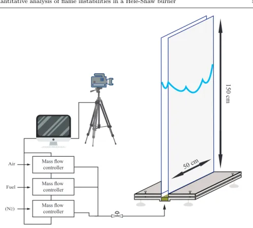
The Hele-Shaw burner consists of two glass plates 50cm wide and 150cm high, sepa-rated by an adjustable gap width that will however in this article be kept constant at 4.7mm (Figure 1). The 50cm width has been chosen to accommodate several unstable wavelengths, typically 100 close to stoichiometry (we actually measure the most unsta-ble wavelength, which is approximatelyλmax∼ 2λc for a Darrieus-Landau dispersion

relationσ ∝ k − k2). The 4.7 mm thickness is a compromise, sufficiently small not to have cells in the thickness, but not very small in order to be far from extinction. The burner is mounted vertically with the inlet gas mixture at the bottom, open at the upper end and it is closed on both vertical sides. The equivalence ratio (φ) and dilution (δ = O2/(O2 + N2)) of the premixed gas are controlled via a PC interface connected to mass-flow regulators Bronkhorst EL-Flow with an accuracy of 1%.

The operating procedure is as follows : after each run, the air flow is opened and maintained until the burner walls have cooled to ambient temperature. The flow of combustible mixture is then adjusted to the desired equivalence ratio and dilution, and a 2D inverted V-flame (a 2D Bunsen flame) is ignited at the top of the burner where it remains anchored thanks to a flow rate in excess compared to the laminar flame velocity. Closing the valve at the bottom of the burner stops the flow and the downwards flame propagation is recorded using a high-speed video camera (Photron FASTCAM SA3). The decrease of the flow is sufficiently smooth so that the deceleration effect is much

(6)

Mass flow controller Mass flow controller Mass flow controller Air Fuel (N2) 150 c m 50 cm

Fig. 1 Experimental set-up

smaller than that of gravity and doesn’t perturb the growth rate measurement. In addition, the acoustic modes of the cell are not observed during the early stages of destabilization where we measure the growth rate.

2.1 Free propagation

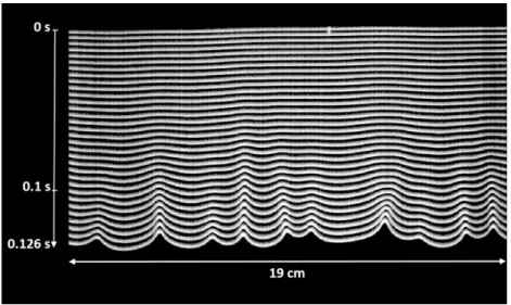
The successive positions and shapes of the flame front drawn on Figure 2 show the natural development of corrugations induced by the intrinsic flame instability. Starting from a quasi planar shape when the flame enters the cell, the flame evolves classically first in a linear stage followed by a crest coalescence period that would end with a stationary regime controlled by coalescence and creation of new cells [13]. Let us note

(7)

that the Sivashinsky equation has exactly the same type of behavior for a large number of unstable modes in the presence of noise.

Fig. 2 Flame front at successive moments, close to the top of the Hele Shaw cell, showing the linear development of the hydrodynamic instability, free propagation, propane-air mixture φ = 0.81.

Discrete Fourier transforms of these profiles confirm this tendency with a linear development of corrugations up to the timet= 0.1s. After that time perturbations with wavenumbers around and slightly smaller thankmaxreach important amplitudes

(see Figure 3).

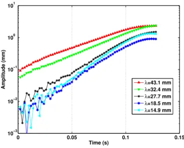
Figure 4 shows the amplitude of different Fourier modes in logarithmic scale versus time, that can be used to measure a linear growth rate with an accuracy of about ±10%.

In Figure 5 (what is actually plotted is the amplitude divided by the wavelength), we illustrate the different regimes in the development of perturbations: a noise dominated regime at low amplitude, a linear regime followed by a non linear saturation. The

(8)

Fig. 3 Temporal evolution of the Fourier transform of the fronts of Figure 2. 0 0.05 0.1 0.15 10−3 10−2 10−1 100 101 Time (s) Amplitude (mm) λ=43.1 mm_{λ=32.4 mm} λ=27.7 mm λ=18.5 mm λ=14.9 mm

Fig. 4 Perturbation amplitude versus time, for the main wavelengths of Figure 3

linear regime is approximated by a straight line (dashed red line in Figure 5), giving the growth rate.

(9)

0 0.05 0.1 0.15 10−5 10−4 10−3 10−2 10−1 Time (s) Amplitude/ λ λ=27.7 mm, σ=48.0 s−1 Linear Non linear Noise

Fig. 5 Perturbation amplitude (divided by λ ) versus time, for λ = 27.7mm

Such an analysis gives access to the linear growth rate for each mode with noticeable amplitude (see Figure 6), but perturbations with wavenumbers slightly higher thankmax

were not easily measurable, as their initial amplitude was too small.

0 0.1 0.2 0.3 0.4 0.5 0.6 0.7 0.8 0 10 20 30 40 50 60 70 80 90 k (mm−1) Growth rate (s −1 )

(10)

2.2 Forced propagation

To bypass the difficulties with the free propagation method, we used a forcing of the inverted V flame at the top of the cell. A plate with periodic indentations was placed a few centimeters above the burner exit, thus forcing the flame response at the desired wavelength.

This plate is placed at the top of the burner as shown in figure 7. Its position relative to the glass plate is a compromise: the perturbation amplitude must not be too large to allow a sufficient growth in the linear regime, but not too small either to overcome the noise and imprecisions of the measures.

Fig. 7 Position of the metallic forcing plate at the top of the burner

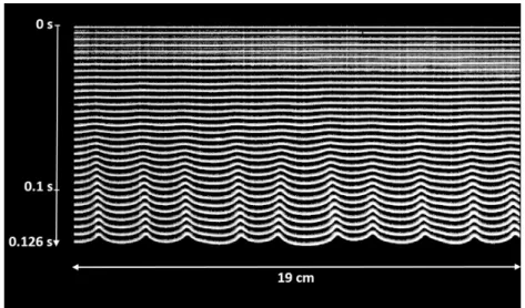
Figure 8, shows the same flame as in Figure 2 (propane-air mixture atφ = 0.81), with a forcing at a wavelength20mm. At the beginning of propagation, the flame is almost plane, then a very regular perturbation appears and a linear evolution is seen up to a time of approximately0.1s. After this time, the non linear effects come into

(11)

play, leading to a complex evolution controlled by the coalescence of the crests present on the front.

Fig. 8 Flame front at successive moments, close to the top of the Hele Shaw cell, showing the linear development of the hydrodynamic instability, forced propagation. propane-air mixture φ = 0.81, forcing wavelength 20mm.

Fourier analysis of the flame front position confirms that the amplitude of the forced perturbation is larger than the one of spontaneous corrugations (Figure 9).

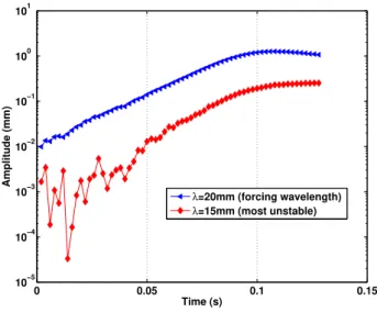
Figure 10 shows the perturbation amplitude corresponding to the forced wavelength in logarithmic scale, compared to the most unstable wavelengthλmaxwhich is present

anyway even without specific forcing. The indentations on the forcing plate are shown in Figure 7, the forcing at a particular wavelength is only approximate, there are also other wavelengths being created. These wavelengths have a much lower initial amplitude, but the amplification is exponential, after some time the most unstable wavelength is always observed. As seen in Figure 10, it is relatively easy to obtain the growth rate corresponding to the forcing wavelength. Let us note however that it

(12)

0 0.2 0.4 0.6 0.8 1 0 0.05 0.1 0.15 0 0.2 0.4 0.6 0.8 1 1.2 k (mm−1) Time (s) Amplitude (mm) λ = 20 mm

Fig. 9 Temporal evolution of the Fourier transform of the fronts of Figure 8.

is difficult to measure growth rates for wavenumbers very far from the most amplified wavenumber. 0 0.05 0.1 0.15 10−5 10−4 10−3 10−2 10−1 100 101 Time (s) Amplitude (mm) λ=20mm (forcing wavelength) λ=15mm (most unstable)

Fig. 10 Perturbation amplitude versus time, for the forced wavelength of Figure 8 and for the most unstable wavelength

(13)

The linear growth rates of the perturbations can be measured in a range of wavenum-bers where σ is typically larger than half its maximal value. Outside this range the measurement of the perturbation is biased by the spontaneous evolution of the most unstable wavelength. Depending on the experiment, the accuracy of each measurement of the linear growth rate can be estimated between 5 to 10% of the measured value, depending on the equivalence ratio and amplitude of initial forcing.

As shown in Figure 11 where growth rates obtained by the forcing method (empty green diamonds) are superimposed to the previous results obtained by free propagation (crosses), the use of forcing represents a marked improvement. Values of growth rates in the descending part of the dispersion relation can now be obtained, the precision is generally better, the most unstable wavelength, an important physical parameter, can be obtained in a much easier way.

We show in Figure 12 the error bars corresponding to the two wavelengths of Figure 10. It can be seen that the typical error for a forced wavelength is much smaller than in an unforced case. In this last case the initial noise present for small times makes it difficult to choose accurately the slope of the line fitting the experimental points, leading to a large error bar on the growth rate.

3 Propane-air and methane-air mixtures

3.1 Growth rates

The results for propane-air flames are plotted for different equivalence ratios in Figure 13. The lines in this figure are best parabolic fits (of the formσ = ak − bk2) through the data [1], the symbols are measurements using the forced propagation method. The theory of the Darrieus Landau instability for flames in tubes has been developed in 1982

(14)

0 0.1 0.2 0.3 0.4 0.5 0.6 0.7 0.8 0.9 0 10 20 30 40 50 60 70 80 90 k (mm−1) Growth rate (s −1 )

Not forced points Forced points Fit by a second order polynomial

Fig. 11 Growth rate vs wavenumber for a propane-air mixture at φ = 0.81, forced propagation (green empty diamonds) superimposed to the free propagation results of figure 6 (black crosses), Fit by a second order polynomial: blue curve

by Pelc´e and Clavin [19] (see also [20] for temperature dependent diffusivities), Matalon and Matkowsky [21], Frankel and Sivashinsky [22]. These articles do not include heat and viscous losses. The two last papers obtain, for zero gravity, the growth rates in the formσ = ak − bk2, whereadepends on gas expansion and laminar flame velocity and bdepends on Lewis number : this is apparently valid for small wavenumbers and for every Lewis number except very low Lewis numbers wherebwould become negative. It seems reasonable to use this type of dispersion relation, also used in the Sivashinsky equation, to fit the experimental measurements when the gravity effects are small, i.e. for sufficiently fast flames.

(15)

0.3 0.32 0.34 0.36 0.38 0.4 0.42 0.44 k (mm-1) 50 52 54 56 58 60 62 64 66 Growth rate (s -1 ) =20 mm =15 mm

Fig. 12 Error bars for the two wavelengths of Figure 10. Propane-air mixture at φ = 0.81

Our measurements are limited to lean or stoichiometric propane-air flames for two reasons. For very rich propane flames (φ > 1.15) the inverted V-flame at the top of the cell is already cellular, preventing us from studying the development of the instability starting from a plane flame. For slightly rich propane-air flames (1.0 <φ < 1.15) we had difficulties anchoring the flame at the top.

Comparing the three equivalence ratios of the figure it appears that stoichiometric flames are much more unstable than lean propane flames. The maximum growth rate for the stoichiometric case is more than three times the value forφ = 0.81. A number of factors lead to this large difference: higher Darrieus Landau instability for φ = 1 (larger laminar flame speed, larger gas expansion) , and diffusive effects producing

(16)

more stable flames in the lean case (the limiting component being propane, with a high Lewis number) [8, 9].

0 0.2 0.4 0.6 0.8 1 1.2 0 20 40 60 80 100 120 140 160 180 200 220 k (mm−1) Growth rate (s −1 ) φ=0.81 φ=0.90 φ=1.00

Fig. 13 Growth rate vs wavenumber for lean and stoichiometric propane-air mixtures.

Figure 14 shows the same type of results for methane-air mixtures (symbols, exper-imental measurements by the forcing method, lines, best parabolic fit). Note that this is the first time that growth rates of methane-air flames are obtained experimentally, the results of the literature being limited to propane-air flames. We have less difficulties for methane than for propane air flames, the results for methane can be obtained even for rich flames.

The maximum growth rate first begins to increase with the equivalence ratio up to φ = 1.1, then sharply decreases for rich flames. On the lean side, the growth rate de-creases less than in the propane case (the limiting component is methane, with a Lewis number close to unity).

(17)

0 0.2 0.4 0.6 0.8 1 1.2 0 20 40 60 80 100 120 140 160 180 200 220 k (mm−1) Growth rate (s −1 ) φ=0.9 φ=1.0 φ=1.1 φ=1.2 φ=1.3

Fig. 14 Growth rate vs wavenumber for methane-air mixtures.

A parabolic fit through such measurements gives access to the maximum growth rateσmaxand to the most amplified wavenumberkmax, We will report these quantities

in the next subsection.

The growth rates of the flames shown in Figures 13 and 14 correspond to downward propagating flames. In the propane case, we compare in Figure 15 the growth rates of upward and downward propagating flames for an equivalence ratio of 0.9 and a cell thickness of 3.5mm(for this thickness the growth rates are slightly smaller). As expected (see [19, 20]), upward propagating flames are more unstable, but the difference is not extremely large. According to Joulin and Sivashinsky [10] the main effect of viscous losses (Saffman Taylor effect) is to act like upward gravity, and thus increase the growth rate. We will see that our measurements in the Hele-Shaw burner are lower than previous measurements, suggesting that the effect of viscous losses is small and much lower than the effect of heat losses, as in the numerical simulations of Kang Baek and Im [18]). In accordance with the theoretical analysis of Joulin and Sivashinsky, we

(18)

find that the primary instability in the Hele-Shaw burner is due to Darrieus-Landau effects. However these effects are reduced by heat losses.

0 0.1 0.2 0.3 0.4 0.5 0.6 0.7 0.8 k (mm-1) 0 20 40 60 80 100 120 140 Growth rate (s -1 ) Propane-air =0.9 thickness 3.5mm

downward propagating flame upward propagating flame

Fig. 15 Growth rate of downward and upward propagating flames for propane-air flames at φ = 0.9

.Figure 15 shows a small effect of buoyancy. With the cell thickness we use (in order to have a quasi two dimensional propagation), flames with a very small burning velocity are quenched, which limits the role of buoyancy. Slow flames can be obtained for very lean or rich flames, but another possibility is to vary the dilution by adding nitrogen. We show in Figure 16 the growth rates of downward propagating methane flames (φ = 1.1) for different dilutions (we recall thatδ = O2/(O2 + N2)is a dilution in oxygen). Reducingδ (adding nitrogen) reduces the flame speed and increases the role of gravity. Let us note however that we were not able to measure growth rates for flames close to the stability threshold far for the most unstable wavelength.

(19)

0 0.2 0.4 0.6 0.8 1 1.2 k (mm-1) 0 20 40 60 80 100 120 140 160 180 200 220 Growth rate (s -1)

Methane =1.1 for different dilutions

=21.0% =20.0% =19.6% =19.1%

Fig. 16 Growth rate of downward propagating methane flames for different dilutions

3.2 Maximum growth rate

In Figure 17, we show for propane and methane-air flames our values for the maximum growth rate σmax in the Hele-Shaw burner versus equivalence ratio compared to the

previous results of the literature for the propane case. Let us first consider the propane case, our values are plotted in red, the values of Clanet and Searby [14] in magenta, the values of Truffaut and Searby [15] in black. These different authors all report the maximum growth rate in a narrow range of equivalence ratio. We have already explained in a previous section the limitations we have in the present Hele-Shaw experiment, let us discuss these two previous articles. In the Clanet Searby case, there is a limitation to very lean propane flames because the method they use to obtain a plane flame (parametric restabilization of the front by an acoustic field) works only for very slow flames. Let us also note that Clanet and Searby do not report actually the maximum growth rate but measure only the growth rate for one wavenumber (expected to be

(20)

close to the maximum). Truffaut and Searby on the other hand, measure the growth of perturbations on oblique flames ; there is apparently a limitation to the rich case in order to anchor the flame.

The values that we measure for the growth rate are of the same order of magnitude as these two previous experiments but seem to have a lower value, particularly com-pared to Truffaut and Searby. We interpret these lower values in the Hele-Shaw cell as being caused by the heat losses to the walls. We include in appendix A measurements of velocity profiles, which seem to indicate that the effective gas expansion in the Hele-Shaw burner is smaller than for flames propagating in tubes.

Unfortunately, we could not obtain growth rates for the same equivalence ratio as the previous measurements. As in the case of propane growth rates decrease quickly for lean flames, the difference between our values in the Hele Shaw cell and measurements of Clanet and Searby [14] and Truffaut and Searby [15] is probably around30%, except close to extinction.

For the methane-air case our experimental measurements are the first ones in the literature. For lean or stoichiometric flames, σmax is close to the value obtained for

propane, then the growth rate decreases on the rich side.

Figure 18 reports the values of kmax, the wavenumber corresponding to the

maxi-mum growth rate. Clanet and Searby do not measure this value since they force their front at one wavelength, but we have added the results of Quinard [8, 9] obtained at the stability threshold (forσmax= 0) for flames highly diluted with nitrogen. This high

dilution leads to smaller values of kmax [14], so it is not surprising that the Quinard

values are smaller, both in the propane and the methane case. For the propane case, the values we obtain (in red) seem smaller than the Truffaut Searby values, but naturally larger than the Quinard values (light blue). For the methane case (green points), we

(21)

0.5 0.6 0.7 0.8 0.9 1 1.1 1.2 1.3 1.4 0 50 100 150 200 250 300 350 400 Φ σmax (s −1 )

Propane this work Methane this work Propane Clanet & Searby Propane Truffaut & Searby

Fig. 17 Maximum growth rate versus equivalence ratio for methane-air and propane-air mix-tures

observe thatkmaxdoes not vary much with the equivalence ratio. The same effect can

be seen (but naturally for lowerkmax) in the experiments of Quinard (blue curve). It

seems also that the values we obtain for methane have a smaller error bar than the propane case.

The values ofkmaxcan be used to obtain the cut-off wavenumberkc≈ 2kmax, leading

to our estimates of the number of unstable modes (typically100close to stoichiometry) in our 50cmburner. The Hele-Shaw burner thickness we use (4.7mm) is close to the cut-off wavelength in this case, since it has been chosen to prevent the appearance of cells in the thickness while being sufficiently large to reduce the heat losses effects.

4 A comparison of the different experimental methods to measure growth rates

We have presented in this article experimental techniques to measure growth rates of the flame hydrodynamic instability in a Hele-Shaw cell. Among the two techniques

(22)

0.4 0.6 0.8 1 1.2 1.4 1.6 0 0.2 0.4 0.6 0.8 1 1.2 1.4 Φ kmax (mm −1 )

Propane this work Methane this work Propane Truffaut & Searby Propane Quinard et al Methane Quinard et al

Fig. 18 wavenumber corresponding to the maximum growth rate versus equivalence ratio for methane-air and propane-air mixtures .

presented here, the forcing method is more precise than the free propagation method. We would like however to compare the forcing method to the methods previously used in the literature to measure growth rates.

Let us start with a general comment. In direct numerical simulations, measurements of growth rates have become relatively common, at least with a one-step chemistry (see for instance [16, 18]). In the experimental literature, on the other hand, we have only two papers, Clanet and Searby [14] and Truffaut and Searby [15], both for propane-air flames.

4.1 Clanet-Searby method

Clanet and Searby use an acoustic field of sufficient amplitude to stabilize a plane flame. They stop the acoustic forcing, perturb the flow with a grid (array of wires), and look

(23)

at the evolution to measure the growth rate. This is the first experiment where growth rates of the hydrodynamic instability were measured. However, this experiment has a number of drawbacks.

1. First of all, the amplitude of the acoustic field must be chosen in order to stabilize the plane flame. For slow flames (< 20 cm/s), e.g. very lean propane-air flames, this is indeed possible, but for relatively fast flames, for instance close to stoichiometry, there is simply no acoustic amplitude able to stabilize the plane flame. On the other hand, the Clanet Searby method would probably also work for flames diluted with nitrogen.

2. The evolution after the acoustic forcing is stopped starts with an important ac-celeration. Normally, a Darrieus Landau instability for any wavenumber generates two modes, a growing mode (the one where we measure growth rates in the present paper) and a decaying mode. With a large initial acceleration the amplitude of the decaying mode is large. As a result the precision of the measurement is low, Clanet and Searby use some fit with two exponentials to measure the growth rate. 3. The initial wavelength is created by a grid in the tube. Apparently Clanet and

Searby have tried grids with several wavelengths, but were only able to report results for one wavelength. It is difficult to know exactly what were the problems at the time (they claim in the article that the method should work for several wavelengths), but let us contrast that with our method with the forcing plate at the top of the cell. If the forcing is too large (so that we have no linear regime) or too small (then we have noise) we simply move the forcing plate and perform a new experiment. It seems difficult to control the initial amplitude in such a way in the Clanet Searby setup.

(24)

4.2 Truffaut-Searby method

Truffaut Searby use an electrostatic forcing on one side of an inverted V-flame and study the development of the perturbation to measure the growth rates. It seems limited to rich flames (to anchor the flame probably) and to relatively large wavenumbers : the authors consider that the two sides of the flame perturb each other for low wavenumbers and do not report the growth rates in this case. It is not obvious anyway that the perturbations on an oblique flame behave exactly in the same way as for plane flames for small wavenumbers. The Truffaut Searby method is interesting compared to Clanet and Searby method since they can control the initial amplitude of the perturbation with the electrostatic forcing in order to stay in the linear regime. This experiment is probably more precise than that of Clanet and Searby, and works for fast flames. There is however the possibility of having vortices created behind the forcing rod which were apparently encountered in some cases [23] and could perturb the measurements.

4.3 Present experiment

In the present experiment, the initial objective was to study flame instability in Hele-Shaw cells quantitatively. It was found possible thanks to the forcing method, which allows us to control the initial amplitude of the perturbation. Compared to the ex-periment of Truffaut and Searby, the method works for lower equivalence ratio in the propane-air case and lower wavenumbers, but until now we were unable to perform measurements for rich propane-air flames. Of course there are two main effects, viscous losses and heat losses, which exist in a Hele-Shaw cell and are not present in a tube. Viscous losses (Saffman-Taylor effects) are supposed to increase the growth rate, heat losses to lower it. We found definitively that the growth rates we measured were lower

(25)

than the two previous experiments, suggesting that heat losses is the dominant effect. Nevertheless except close to extinction, our values of growth rates are not completely different from the previous experiments. The general form of the dispersion relation is also the one typical of a Darrieus-Landau instability.

5 Conclusion

We have shown in this article that a Hele-Shaw burner, a configuration proposed twenty years ago by Joulin and Sivashinsky, can be used for a quantitative analysis of flame instabilities. The instability in a Hele Shaw cell, although apparently smaller because of heat losses, is close to the usual Darrieus Landau instability observed in tubes. Because of the quasi two dimensional geometry, the experiments are relatively easy to perform. Very unstable flames (hundred of unstable modes, a situation typical of high pressure premixed flames) can be obtained here at atmospheric pressure. It was possible to obtain a plane flame at the top of the burner and study the development of perturba-tions by a simple image analysis. In this article, we have insisted on the experimental technique needed to obtain quantitative results. We plan to study in future papers if our results are comparable to existing experiments in terms of Markstein length and if the dispersion relation measured here can help in the non linear modelling of the front propagation.

6 Acknowledgements

(26)

7 Compliance with Ethical Statements

Funding : This work was supported by the French National Research Agency (project PDF) under agreement ANR-14-CE05-0006. The project leading to this publication has received funding from Excellence Initiative of Aix-Marseille University - A*MIDEX, a French "Investissements d’Avenir" programme. It has been carried out in the framework of the Labex MEC.

Conflict of Interest: The authors declare that they have no conflict of interest.

References

1. P. Clavin and G. Searby. Combustion waves and fronts in flows, Cambridge University Press, Cambridge (2016).

2. H. Kobayashi, H. Kawazoe, Flame instability effects on the smallest wrinkling scale and burning velocity of high-pressure turbulent premixed flames, Proceedings of the Combustion Institute , 28:375–382, (2000).

3. V. R. Savarianandam, C.J. Lawn, Burning velocity of premixed turbulent flames in the weakly wrinkled regime, Combust. Flame , 146:1-18, (2006).

4. N. Fogla, F. Creta, M.Matalon. The turbulent flame speed for low-to-moderate turbulence intensities: Hydrodynamic theory vs. experiments, Combust. Flame , 175:155-169, (2017).

5. G.I. Sivashinsky, Nonlinear Analysis of Hydrodynamic Instability in Laminar flames I. Derivation of Basic Equations, Acta Astronautica, 4:111, (1977). 6. C. Almarcha, B. Denet, J. Quinard, Premixed flames propagating freely in tubes,

(27)

7. Y. A. Gostintsev, V. E. Fortov, and Y. V. Shatskikh, Self-Similar Propagation Law and Fractal Structure of the Surface of a Free Expanding Turbulent Spherical Flame, Doklady Physical Chemistry, 397:141-144, (2004).

8. J. Quinard, Limites de stabilité des structures cellulaires dans les flammes de prémélange, étude expérimentale, Thèse d’état, Marseille (1984).

9. J. Quinard, G. Searby, B. Denet and J. Gra˜na-Otero, Self-Turbulent Flame Speeds, Flow Turbulence Combust. , 89:231-247, (2012).

10. G. Joulin, G.I. Sivashinsky, Influence of Momentum and Heat Losses on the Large-Scale Stability of Quasi-2D Premixed Flames, Combust. Sci. and Tech., 98:11- 23., (1994).

11. J. Sharif, M. Abid, and P. D. Ronney, Premixed-Gas Flame Propagation in Hele-Shaw Cells, Spring Technical Meeting, Joint US Sections, Combustion Institute, Washington, DC, 1999. http ://ntrs.nasa.gov/archive/nasa/casi.ntrs.nasa.gov/20000005014.pdf. (1999). 12. J. Wongwiwat, J. Gross, P. Ronney, Flame Propagation in Narrow Channels at

Varying Lewis Number, 25th ICDERS Leeds, UK August 2 – 7, (2015).

13. C. Almarcha, J. Quinard, B. Denet, E. Al-Sarraf, J. M. Laugier, and E. Villermaux. Experimental Two Dimensional Cellular Flames, Physics of Fluids, 27:091110, (2015).

14. C. Clanet, G. Searby, First experimental study of the Darrieus-Landau instability, Phys. Rev. Lett., 80:3867-3870., (1998).

15. J.M. Truffaut, G. Searby, Study of the Darrieus-Landau instability on an inverted-’V’ flame, and measurement of the Markstein number, Combust. Sci. and Tech., 149:35-52., (1999).

(28)

16. B. Denet and P. Haldenwang. A numerical study of premixed flames Darrieus-Landau instability, Combust. Sci. and Tech., 104:143–167, (1995).

17. S.H. Kang, H. G. Im, and S. W. Baek. A Computational Study of Saffman-Taylor Instability in Premixed Flames, Combustion Theory and Modelling, 7:343-363, (2003).

18. S.H. Kang, S. W. Baek and H. G. Im, Effects of heat and momentum losses on the stability of premixed flames in a narrow channel, Combustion Theory and Modelling, 10:4659-681, (2006).

19. P. Pelc´e and P. Clavin, Influence of hydrodynamics and diffusion upon the stabil-ity limits of laminar premixed flames, Journal of Fluid Mechanics, 124, 219-237, (1982).

20. P. Clavin and P. Garcia, The influence of the temperature dependence of diffusivi-ties on the dynamics. Journal de Mécanique Théorique et Appliquée, 2(2), 245-263, (1983).

21. M. Matalon and B. J. Matkowsky, Flames as gasdynamic discontinuities. Journal of Fluid Mechanics, 124, 239-259, (1982).

22. M.L. Frankel and G.I. Sivashinsky, The effect of viscosity on hydrodynamic stability of a plane flame front, Combust. Sci. and Tech., 29(3-6), 207-224, (1982).

23. J.M. Truffaut, Etude expérimentale de l’origine du bruit émis par les flammes de chalumeaux. 1998. Thèse de doctorat. Université de Provence-Aix-Marseille I, (1998).

24. M.L. Frankel and G.I. Sivashinsky, On effects due to thermal expansion and Lewis number in spherical flame propagation, Combust. Sci. and Tech., 31(3-4): 131-138, (1983).

(29)

25. D.G. Goodwin, H.K. Moffat and R.L. Speth, Cantera: An object-oriented soft-ware toolkit for chemical kinetics, thermodynamics, and transport processes. http://www.cantera.org, Version 2.3.0. doi:10.5281/zenodo.170284, (2017). 26. Chemical-Kinetic Mechanisms for Combustion Applications, San Diego

Mecha-nism web page, Mechanical and Aerospace Engineering (Combustion Research), University of California at San Diego, http://combustion.ucsd.edu (2017).

Appendix A Gas expansion

We have shown in this article that the growth rates of the hydrodynamic instability in the Hele-Shaw cell, are generally smaller than those in a tube, which suggests that heat losses play a role. It would be interesting to measure the temperature profile in the burner, but this is a difficult task. We show in this section that by measuring the velocity field on both sides of the flame , burnt and fresh gases, by a PIV technique using cesium oxide particles as seeding material, experimental values of the expansion ratio E can be obtained. It is known [24] that the normal mass flux is not exactly conserved across the flame, so measuring the velocity jump between fresh and burnt gases does not give exactly the expansion ratio, however for our purpose we only need approximate values of the expansion ratio (these values will be used to discuss in more detail the Darrieus Landau instability in the Hele-Shaw burner in future papers). Figure 19 (propaneφ = 0.9) shows the velocity field in the fresh and burnt gases and the normals at different positions on the front in a small cell (60 cm×1.5 cm×5 mm). We use a smaller cell here in order to reduce the presence of cusps on the front, the heat losses however are slightly increased.

(30)

2 4 6 8

x

(

mm

)

0 2 4 6 8 10

y

(

mm

)

Fig. 19 Velocity field and normals at different positions on the front in a small cell 60 cm×1.5 cm×5 mm

Figure 20 shows the normal velocity profile deduced from the previous figure at different positions on the front. Taking the average of velocity ratio between burnt and fresh gases in the different curves of Figure 20, we obtain a gas expansionE= 6.1 ±0.25, which can be compared to the value obtained by Cantera [25] with a San Diego mech-anism [26]E= 7.57 for propane atφ = 0.9. As expected the value obtained experi-mentally is slightly lower, probably because of heat losses. The typical thickness of the velocity profile is also close to the one given by complex chemistry, shown as a dashed line on the figure. Note that these profiles are obtained by PIV, it is possible that out-of-plane effects exist in this configuration. It seems that as suggested by Joulin and Sivashinsky [10] heat losses have an important role in the Hele-Shaw cell, which

(31)

could be described by a lower gas expansion. 0.0 0.2 0.4 0.6 0.8 1.0 1.2