History effect in fatigue crack growth under mixed-mode loading conditions

HAL Id: hal-00417887

https://hal.archives-ouvertes.fr/hal-00417887

Submitted on 17 Sep 2009

HAL is a multi-disciplinary open access archive for the deposit and dissemination of sci-entific research documents, whether they are pub-lished or not. The documents may come from teaching and research institutions in France or

L’archive ouverte pluridisciplinaire HAL, est destinée au dépôt et à la diffusion de documents scientifiques de niveau recherche, publiés ou non, émanant des établissements d’enseignement et de recherche français ou étrangers, des laboratoires

History effect in fatigue crack growth under mixed-mode

loading conditions

Pierre-Yves Decreuse, Sylvie Pommier, Laetitia Gentot, Stéphane Pattofatto

To cite this version:

Pierre-Yves Decreuse, Sylvie Pommier, Laetitia Gentot, Stéphane Pattofatto. History effect in fatigue crack growth under mixed-mode loading conditions. International Journal of Fatigue, Elsevier, 2009, 31 (11-12), pp.1733-1741. �10.1016/j.ijfatigue.2009.03.014�. �hal-00417887�

H

ISTORY EFFECT IN FATIGUE CRACK GROWTH UNDER MIXED MODE LOADING CONDITIONS

P.Y. Decreuse, S. Pommier, L. Gentot, S. Pattofatto

LMT-Cachan (ENS Cachan/CNRS/UPMC/UniverSud Paris), 61, avenue du Président Wilson, 94235 Cachan, France

Abstract: Plastic deformation within the crack tip region introduces internal stresses that modify

subsequent behaviour of the crack and are at the origin of history effects in fatigue crack growth. Consequently, fatigue crack growth models should include plasticity induced history effects. A model was developed and validated for mode I fatigue crack growth under variable amplitude loading conditions. The purpose of this study was to extend this model to mixed mode loading conditions. Finite element analyses are commonly employed to model crack tip plasticity and were shown to give very satisfactory results. However, if millions of cycles need to be modelled to predict the fatigue behaviour of an industrial component, the finite element method becomes computationally too expensive. By employing a multiscale approach, the local results of FE computations can be brought to the global scale. This approach consists of partitioning the velocity field at the crack tip into plastic and elastic parts. Each part is partitioned into mode I and mode II components, and finally each component is the product of a reference spatial field and an intensity factor. The intensity factor of the mode I and mode II plastic parts of the velocity fields, denoted by dρI/dt and dρII/dt, allow measuring mixed-mode plasticity in the crack tip region at the global scale.

Evolutions of dρI/dt and dρII/dt, generated using the FE method for various loading histories, enable

the identification of an empirical cyclic elastic-plastic constitutive model for the crack tip region at the global scale. Once identified, this empirical model can be employed, with no need of additional FE computations, resulting in faster computations. With the additional hypothesis that the fatigue

crack growth rate and direction can be determined from mixed mode crack tip plasticity (dρI/dt and

dρII/dt), it becomes possible to predict fatigue crack growth under I/II mixed mode and variable

amplitude loading conditions. To compare the predictions of this model with experiments, an asymmetric four point bend test system was set-up. It allows applying any mixed mode loading case from a pure mode I condition to a pure mode II. Initial experimental results showed an increase of the mode I fatigue crack growth rate after the application of a set of mode II overload cycles.

Keywords: fatigue crack growth, mixed mode, plasticity, model, finite element analyses Nomenclature

FE Finite element method

LEFM Linear Elastic Fracture Mechanics

∞ I

K , K_II∞ Mode I and mode II nominal stress intensity factors

e

I

u , u e_II Mode I and mode II elastic reference displacement fields

c

I

u , u c_II Mode I and mode II complementary reference displacement fields

I

K~ ,K~ _II Mode I and mode II pseudo-elastic intensity factors

I

ρ , ρ_II Mode I and mode II plastic intensity factors

X I

K , K_IIX Centre of the elastic domain, global measure of internal stresses at crack tip.

1. Introduction

Crack tip plasticity is known to be at the origin of memory effects in fatigue of metallic materials [1-8], which has posed difficulties in modelling fatigue crack growth under variable amplitude loadings. Moreover, history effects are closely related to the cyclic elastic-plastic behaviour of the material [9-10], which makes the use of a universal model questionable. The application of a mode I overload delays the fatigue crack growth. The overload yields the material ahead of the crack tip creating compressive residual stresses in the overload’s plastic zone. As a consequence, the efficiency of subsequent fatigue cycles is reduced and the rate of fatigue crack growth is decreased. This is commonly known as plasticity-induced crack closure [3]. These history effects are also present under variable amplitude mixed mode loading conditions [12-22].

For instance, Dahlin & Olsson [14] performed experiments to determine the influence periodic mode II loading had on mode I cycles. They concluded that mode II cycles decrease the fatigue crack growth rate during mode I cycles. Similar observations were made by Gau & Upul [13] for low alloyed steel. For the same type of experiments, Nayeb-Hashemi & Taslim [18] found a transient acceleration just after the loading application.

predict the direction of the crack under mixed mode loading. There is general agreement in the literature that plasticity in the crack tip region and induced history effects modify both the growth direction and the fatigue crack growth rate. This paper aims at proposing a global model for describing the evolution of crack tip plasticity and internal stresses when non-proportional mixed mode loading conditions are encountered. In the future this model could be employed in a fatigue crack growth criterion.

Finite element methods are useful for analyzing crack tip plasticity under various loading conditions [4,9-11, 19-22]. In particular, FE analyses allow accounting for rather complex material constitutive behaviour [9,10]. However, the simulation of mode I or mixed-mode fatigue crack growth by elastic-plastic finite element computations leads to huge computation cost. In order to model service conditions in engineering applications, the computations become even more expensive, because real components often have fatigue lives of millions cycles, and cracks do not generally remain planar. The objective of the proposed methodology is to combine the precision of local finite element computations with the rapidity of a global approach [25-27].

2. Material and experiments.

The studied material is a S355NL steel used for marine applications. Its chemical composition is reported in Table 1. The grains are equi-axed and their size is typically around 20 micrometers.

Table 1: Chemical composition of the S355NL steel in weight %.

C (%) Mn (%) P (%) S (%) Si (%) Al (%) Cr (%) Cu (%) Ni (%)

0.12 1.46 0.016 0.01 0.44 0.041 0.02 0.01 0.01

Cylindrical specimens were cut from a 16 mm thick metal sheet in order to characterize the elastic-plastic constitutive behaviour of the S255NL steel. Strain controlled push-pull tests were performed with increasing strain amplitude. The material displayed kinematic hardening and the isotropic hardening was negligible. The cyclic elastic-plastic behaviour of this material [29] was modelled using the Von Mises criterion and the non-linear kinematic hardening law of Armstrong and Frederick, standard in Abaqus 6.5. The material parameters used for the simulations are reported in Table 2. A reasonable agreement is found between experiments and simulations (Fig. 1), but it might be useful to improve the description of the kinematic hardening rule in the future.

This material constitutive behaviour is used in the following for the finite element simulations of crack tip plasticity under mixed mode conditions.

Table 2: Parameters of the elastic-plastic constitutive behaviour employed for the simulations.

Young’s modulus (GPa) 180000

Poisson’s ratio 0.3

Initial yield stress Ro (MPa) 178

Kinematic hardening parameter C (GPa) 100

Kinematic hardening rate γ 500

(a) (b)

Figure 1: Strain controlled push pull test. Comparison between experimental and simulated

stress-strain curves at Rε=-1 and εmax= 0.5% (a) or εmax= 0.9% (b). Symbols: Experiments, lines: simulations.

Four point bending specimens were also cut from the same material source, with a thickness of 5 mm, a length of 180 mm and a width of 30 mm. A notch with length 8 mm and thickness 1.5 mm was created and the specimens were pre-cracked under mode I conditions with a stress ratio of 0.1.

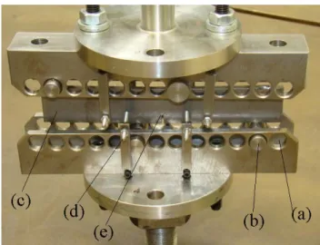
The specimens were mounted on a non-symmetric four point bend test system. Load was applied to the sample through roller bearings (Fig. 2). When the bearings were placed symmetrically with

respect to the crack plane, a mode I stress intensity factor is achieved. On the contrary an anti-symmetric position creates a mode II stress intensity factor. The relations between the bending

moment and K , and between the shear force and _I∞ K , were determined using solutions from a _II∞

fracture mechanics handbook [30]. Any intermediate position of the bearings corresponds to a given proportional mixed mode loading condition (Fig. 2). Crack extension was determined using potential drop measurements. The relation between the crack length and the potential drop was calibrated using both the initial and final crack dimensions and intermediate crack tip positions determined using digital image correlations (DIC). As a matter of fact, during the experiments images of the surface were taken periodically to determine the crack tip position and deviation of the crack growth plane.

Figure 2: Non-symmetric four point bending system in an intermediate position. (a) seating for the

roller bearings, (b) axles of the roller bearings adjusted to the seatings, (c) sample, (d) lateral positioning, (e) initial notch.

First, a specimen was tested to failure under pure mode I loading to generate a reference da/dN-ΔK curve. Second, a crack was grown under mode I conditions to a length of 12 mm. At this point,

m MPa K_I =10

Δ ∞

. The bearings were displaced so as to apply a mode II load and the load was

adjusted such that ΔK_II∞ =20MPa m and R=0.1. No further fatigue crack growth was observed,

even after 500000 mode II cycles. The conclusion of this first experiment was that a mode II

loading of ΔK_II∞ =20MPa m was not sufficient to promote fatigue crack growth after mode I

Third, a crack was grown to a length of 12 mm under the same mode I conditions as in the second experiment. Then the bearings were displaced to apply either one, ten or fifty mode II cycles

and the load adjusted such that ΔK_II∞ =20MPa m . Then the bearings were displaced again so as to

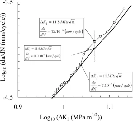
apply mode I nominal fatigue cycles, and the crack was grown again until fracture. It was observed in this case that the application of ten mode II cycles accelerated the crack (circles in Fig. 3) compared to the pure mode I fatigue crack growth experiment (thick line in Fig. 3). The increase of the fatigue crack growth rate was moderate (by about 20%) but the recovery length was large (around 3 mm). This effect is moderate but significant. The increase of the crack growth rate after 50 mode II cycles is similar to that obtained after 10 mode II cycles. That obtained after only one mode II cycle was negligible. During these experiments, a slight deviation of the crack growth plane was observed just after the application of mode II cycles. However, this deviation was

neglected for the calculation of K . _I∞

Figure 3: Crack growth rate in a Paris diagram as measured in the S355NL steel at room

temperature. The thick line correspond to a reference mode I fatigue crack growth experiment with R=0.1. The dots corresponds to a mode I fatigue crack growth before and after the application of

Complementary experiments are planned in order to better characterize the mixed mode fatigue crack behaviour in the S355NL steel and related history effects. However, it can be concluded from this very first set of experiments that, for the experimental conditions tested, mode II cycles do not promote fatigue crack growth, but are at the origin of a history effect on mode I fatigue crack growth.

However, this history effect is detrimental, while various authors [14, 15, 21, 22] have found a retardation effect of a mode II cycle on mode I fatigue crack growth. In particular, Dahlin & Olsson [14] made different experiments to study the influence of periodic mode II loading on mode I fatigue crack growth in a low alloyed steel, according to the stress ratio R of mode I cycles. First, among five different experimental conditions, only one shows an acceleration of 12% of the crack

growth rate. In this case, the stress ratio and ΔKII were high (R=0.58, ΔKII=30 MPa.m1/2) compared

with our experimental conditions (R=0.1, ΔKI=10 MPa.m1/2). The other experiments were

performed with a stress ratio comparable to that used in our experiments (R=0.1). Contrary to the

experimental results in Fig.3, Dahlin & Olsson [14] observed a decrease of the crack growth rate,

regardless of the number of periodic mode II loadings.

Quite the opposite, Nayeb-Hashemi and Taslim[18] obtained only a transient acceleration of the

crack after the application of a single mode II cycle, without any retardation. Their results are similar to those plotted in Fig. 3.

As a conclusion, predicting history effects in mixed mode conditions is not straightforward. History effects are suspected to be a function of the material, the stress ratio, the overload ratio, etc… Therefore, having a method to predict history effects under mixed mode conditions will be useful to design interesting loading schemes and to setup the experiment to elucidate suspected effects. In the following, such a method is developed and employed to simulate the evolution of crack tip plasticity for loading conditions equivalent to that used in the experiments (Fig. 3).

3. Modelling

Previously, a model was developed and validated for mode I fatigue crack growth under variable amplitude loadings conditions [25,26]. It was able to model fatigue crack growth including plasticity induced history effects. A natural evolution for this model should be to extend it to mixed

mode loading conditions. Many authors [11-18] have researched this open problem, and all agree

and the growth rate of a fatigue crack.

Moreover, it was shown by Sander and Richards [21,22] and Doquet et al. [19], respectively, that suitable FE computations allow successful prediction of the crack growth rate [21,22] and direction [19] under non-proportional mixed mode conditions.

As a matter of fact, in mixed mode conditions, as in mode I conditions, cyclic plasticity within the crack tip region lies at the origin of internal stresses that superimpose on the applied stresses and modify the behaviour of the crack. The FE method allows determining local loading conditions within the crack tip region that can then be used in a local crack growth criterion. For instance, Doquet et al [19] used elastic-plastic FE computations to determine stresses and strains around the crack tip for sequential mode I / mode II cycles. The average stress and strain fields over a critical distance from the crack tip were then computed and used to determine the plane for which the fatigue damage rate per cycle is the highest. The damage criterion was, for instance, a function of the normal stress amplitude. Other criteria are also used according to the material and the damage mechanism. It allows determination of the crack propagation plane. This approach was shown to predict successfully the conditions for which the fatigue crack bifurcates for sequential mode I / mode II loading conditions.

Unfortunately, these approaches remain limited in practice because of the huge costs of the implementation of FE models an of elastic-plastic cracked body and of their analysis in fatigue. Moreover, in an industrial context, a fatigue crack growth model may have to handle millions of cycles, which imposes the use of simplified methods. Therefore, a global model, which would be easier to handle than a local one, is desired for this problem.

3.1 The multiscale approach

The main advantage of using the FE method is that it makes possible the use of complex material constitutive behaviours required to compute the details of the evolution of plastic deformation, residual stresses, stress range, etc… within and around the crack tip region for a stationary or moving crack tip [9,10].

The local FE results are then brought to the global scale using a multiscale approach tailored for crack problems [25-27]. The global data generated by the post-treatment of FE computations are

region. This model is incremental to facilitate its use in variable amplitude fatigue. For instance, in

mode I, the global plasticity rate, dρ_I dt, within the crack tip region is a function of the nominal

loading rate dK_I∞ dt and the state of a set of internal variables [25-27]. In addition, a proportional

growth law between the rate da dt of production of cracked area per unit length of the crack front

and dρ_I dt, allows prediction of the crack growth rate. Finally, the model is a set of ten scalar

partial differential equations.

The procedure to identify the parameters in the model f requires knowledge of the material

cyclic elastic-plastic behaviour. It is performed using the FE method and is fully automatic. The identification of the parameter in the growth law requires the results of a constant amplitude fatigue crack growth experiment. More details about the global model development can be found in [25].

Once identified, the global model can be used to predict the fatigue crack growth rate for variable amplitude loadings schemes. It accounts for plasticity induced history effects and is cheap in computation cost. The objective is now to extend this approach for non-proportional I/II mixed mode problems.

3.1.1 Basis

For plane problems, the velocity field within the crack tip region in I/II mixed mode conditions is partitioned into mode I and mode II components that correspond to the symmetric and anti-symmetric parts of the displacement field with respect to the crack plane, respectively. In LEFM,

the velocity field is then approximated by the product of spatial reference fields ( e

I

u and e

II

u ) and

their nominal stress intensity factors rates (K& and _I∞ K&_II∞ ) (Eq. 1).

( )

P v

( )

tip K u

( )

P K u

( )

P

v − ≈ &_I∞ e_I − &_II∞ e_II (1)

In order to extend this approach to an elastic-plastic behaviour, two additional spatial reference

fields ( c I

u and c

II

u ) and their intensity factor rates (ρ& and _I ρ& ) are used to describe the velocity II

field in the crack tip region (Eq. 2).

( )

P v

( )

tip K u

( )

P u

( )

P K u

( )

P u

( )

P

The additional spatial reference fields ( c I

u and c

II

u ) are constructed to be non-dimensional such

that the intensity factor rates (ρ& and _I ρ& ) are equivalent to the rate of the crack tip opening _II

displacement and the crack tip sliding displacement

(

dCTOD dt, dCTSD dt

)

, respectively.

At this point, the velocity field in the crack tip region is fully defined by a set of global variables,

( )

tip

v , the crack tip velocity, and the intensity factor rates of the elastic and plastic parts of each

mode

(

K~&_I,K~&_II,ρ&_I,ρ&_II

)

.

Velocity fields v

( )

P for stationary or moving cracks in elastic-plastic conditions are calculated using the finite element method for various load histories. A POD based routine is then used to

approach v

( )

P either by Eq. 2 (elastic approximation) or by Eq. 3 (elastic-plastic approximation)

and to determine the related errors (Eq. 3 and 4)

( ) ( )

( )

( )

(

)

(

( ) ( )

)

_⎟⎟ ⎠ ⎞ ⎜ ⎜ ⎝ ⎛ − ⎟ ⎟ ⎠ ⎞ ⎜ ⎜ ⎝ ⎛ − − − =

∑

∑

∈ ∈ ∞ ∞ D P i D P i e II II i e I I i e i i tip v P v P u K P u K tip v P v C & & 2 2 (3)

( ) ( )

( )

( )

( )

( )

(

)

∑

(

( ) ( )

)

∑

∈ ∈ − ⎟ ⎟ ⎠ ⎞ ⎜ ⎜ ⎝ ⎛ − − − − − = D P i D P i c II II i e II II i c I I i e I I i ep i i tip v P v P u P u K P u P u K tip v P v

C ~& ρ& ~& ρ& 2 2(4)

During a time increment, the crack tip region (D) is assumed to behave essentially elastically if the elastic approximation of v

( )

P is just as precise as the elastic-plastic one

(

C_e −C_ep ≤C_th

)

. On the

contrary, if the approximation of v

( )

P is improved by the use of two additional spatial reference

fields ( c I

u and u ) and their intensity factor rates (c_II ρ& and I ρ& ), the crack tip region plastically II

deforms.

3.1.2 Implementation

2D finite element simulations were performed using Abaqus 6.5. Linear plane strain elements were used to mesh a quasi infinite sheet (20m x 20m) containing a central crack with a length of 2a=60mm. The mesh was highly refined around the crack tip with a mesh size of 3 μm at 10μm from the crack tip (Figure 4). The “crack tip region” was defined as the set of elements at a distance below 1mm from the crack tip.

(a) (b)

Figure 4: Finite elements mesh, (a) increasing mesh refinement around the crack tip, (b) detail of

the mesh around the crack tip.

The first step of the procedure consists in determining the two reference elastic fields, e

I

u and

e

II

u , from elastic finite element computations for which the nominal stress intensity factors were

m MPa

KI∞ =1 and KII∞ =1MPa m , respectively.

The complementary fields, c

I

u and u , were then determined using elastic-plastic FE c_II

computations and the material constitutive law (Table 2),. To construct c

I

u for instance, the

following procedure was used. A monotonic mode I tensile phase is simulated using the FE method. The displacement increment Δu

( )

P =u

(

P,t₂

) (

−u P,t₁

)

is computed at each point of the model during the last time increment of that loading phase. Then the displacement field Δu

( )

P during that increment is projected onto the mode I elastic reference field, which allows computation of the variation of its intensity factor during the increment :

( )

( )

( ) ( )

( ) ( )

∫

∫

⋅ ⋅ Δ = − D e I e I D e I I I P u P u P u P u t K t K~ ₂ ~ ₁ (5)

The remainder of the displacement field (see Eq. 1) is then computed:

( )

P u

( )

P

(

K

( )

t K

( )

t

)

u

( )

P uR =Δ − ~I 2 −~I 1 eI

Δ (6)

And then made non-dimensional soρ& could be read as the average relative mode I displacement _I

( )

( )

(

)

(

)

(

)

∫

∫

= = = = − = − = Δ = _{r mm} m r R y R y mm r m r R c I r u r u m P u P u ₁ 10 1 10 , , 1 . μ μ π θ π θ μ (7)

The same procedure was employed in mode II. Once these preliminary computations have been

performed for a given material constitutive equation, ue_I, ue_II, uc_I and uc_II are defined and can be employed for any cyclic mixed mode loading.

In the following, various mixed mode conditions are simulated using the FE method. For each

time increment

(

t_n+1−t_n

)

, the computed displacement field during the time increment

(

) (

)

[

u P,tn+1 −u P,tn

]

is stored and partitioned into mode I

[

uI

(

P,tn+1

)

−uI

(

P,tn

)

]

and mode II

components

[

u_II

(

P,t_n+1

)

−u_II

(

P,t_n

)

]

(e.g. symmetric and anti-symmetric parts). Then the four intensity factor variations during the increment are determined, as shown in equations 8 to 11 :

( )

( )

[

(

)

(

)

]

( )

( ) ( )

∫

∫

⋅ ⋅ − = − + + D e I e I D e I n I n I I n I P u P u P u t P u t P u t K t K , , ~ ~ 1 1 (8)

( )

( )

[

(

)

(

)

]

( )

( ) ( )

∫

∫

⋅ ⋅ − = − + + D c I c I D c I n I n I I n I P u P u P u t P u t P u t t , , ₁ 1 ρ ρ (9)

( )

( )

[

(

)

(

)

]

( )

( )

( )

∫

∫

⋅ ⋅ − = − + + D e II e II D e II n II n II II n II P u P u P u t P u t P u t K t K , , ~ ~ 1 1 (10)

( )

( )

[

(

)

_{( )}

(

_{( )}

)

]

( )

∫

∫

⋅ ⋅ − = − + + D c II c II D c II n II n II II n II P u P u P u t P u t P u t t , , ₁ 1 ρ ρ (11)

The mean least square errors, C_e and C , between the computed displacement field and the _ep

the elastic-plastic approximation was always below 10% whatever the mode mixity and the history provided that the equivalent stress intensity factor used in the simulations is reasonable (e.g. below

50 MPa.m1/2 for this steel). This procedure was fully automated using a python script in Abaqus and

requires a few minutes to post-treat FE simulations.

3.1.3 Results

Various loading histories were simulated. A few examples are given in Fig. 5 to illustrate how

I

ρ and ρ_II (Fig. 5b), that measure crack tip plasticity at the global scale, evolve according to the

mixed mode loading conditions (Fig. 5a). Three steps are applied in each case. The same loading

conditions are applied during the two first steps (Fig. 5a). For the first case, though K is kept _I∞

constant during the last step, both ρ_II and ρ_I increase when K increases. For the second case, _II∞ both ρ_II and ρ_I vary when K is kept constant and _II∞ K increases. On the contrary, in the fourth _I∞ case, ρ_I is nearly constant, while both K and ∞_II K vary. And finally in the third case, during the _I∞ last step of the computation, K and _II∞ K are both decreasing but _I∞ K remains positive. In this ∞_I case, though K is decreasing, _I∞ ρ_I increases. In other words, the crack plastically blunts during the unloading phase.

(a) (b)

These results are qualitatively consistent with experimental and numerical results from Dahlin and Olsson [14] who have shown that focus should not be placed only on “ranges”. The behaviour of a crack in mixed-mode conditions differs significantly whether or not a static mode I load is superimposed with a cyclic mode II load [14].

3.2 Model

The aim is now to find a set of simple variational evolution equations that would reproduce FE results such as those in Fig. 5, and, once identified for a given material, could then be employed to predict mixed mode plasticity at the crack tip in preference to expensive FE computations.

For this purpose a global cyclic elastic-plastic model for the crack tip region is built. It contains a yield criterion, a flow rule and a hardening rule. It is analogous to a plasticity model except that it applies to cracks. Details about this model can be found in [31].

3.2.1 Yield criterion

Using the multiscale approach detailed in §3.1 it is possible to apply a given load history to the crack, and then explore radiating loading directions (Fig. 6a). In each direction, the “yield” threshold is determined as the point above which the approximation of the velocity field by Eq. 2 is better than an elastic approximation (Eq. 1). When the yield point is reached, ρ& and _I ρ& are non _II negligible. It is therefore possible to construct numerically the elastic domain for the crack tip region (Fig. 6b) and its evolution during loading (Fig. 6c).

Using the FE method, it is found that the size and the shape of this domain remains the same

during loading (Fig. 6c). The elastic domain is roughly an ellipsis in a K and _II∞ K diagram. _I∞

However, its center evolves during loading (Fig. 6c). The displacement of the center of the elastic domain is due to the growth of internal stresses within the crack tip region because of the

development of a plastic strain gradient at crack tip. The center of this domain, denoted by K and _IIX

X I

K , is therefore introduced as an internal variable in the model. K and _IIX K stand, at the global _IX

(a) (b)

(c)

Figure 6: Construction of the global yield locus of the crack tip region. (a) typical loading histories

applied during FE computations. (b) dots: yield points as determined using the FE method for each radial loading direction. Solid lines: yield locus as defined from the generalized Von Mises criterion (Eq. 12). (c) Yield locus evolution during loading (dots : from FE, solid lines : Eq. 12).

About 2 hours of FE computations are required to construct each yield surface.

Inside the elastic domain, the crack tip region behaves essentially elastically. Therefore the

Westergaard equations apply (provided that K −_I∞ K_IX and K −_II∞ K_IIX are used) and can be used to determine an analytical expression of the elastic shear energy inside any circular domain around the crack tip. At the local scale the material obeys the Von Mises yield criterion, which stems from a critical shear elastic energy density. Therefore, a critical shear elastic energy criterion in the crack tip region was expected to be a suitable yield criterion at the global scale. The generalized Von

Fig. 6c) and it sums up into a very simple equation (Eq. 12). The elastic domain, defined by f , has _Y a size controlled by the adjustable parameter K and a fixed aspect ratio _IY K_IIY KY_I function of the Poisson’s ratio of the material (Eq. 13).

(

) (

)

2 2

(

) ( )

2 2 , , , Y II IIX YI II Y I X I I X I X II I II Y K K K K K K K K K K K f _⎟⎟ − − ⎠ ⎞ ⎜⎜ ⎝ ⎛ + − = ∞ ∞ ∞ ∞ (12) 2 2 16 16 19 16 16 7 ν ν ν ν + − + − = Y I Y II K K , if ν =0.3 : K_IIY KY_I ≈0.48 (13)

3.2.2 Flow rule, hardening rule and equations of the model.

A flow rule and a hardening rule were then introduced. The normality flow rule was adopted (in a GI, GII diagram rather than in a KI, KII). This flow rule determines the direction of dρI and dρII

(Eq. 17) once the yield surface is reached.

Finally, we also assume as a hardening rule, that the displacement of the center of the yield

surface coincides with the plastic flow direction, which yields : dK_IIX = pdρ_II and dK_IX = pdρ_I . To summarize briefly, the first elements of a global variational formulation of the mixed-mode cyclic elastic-plastic behaviour of the crack tip region were gathered. First, at the global scale, plasticity in the crack tip region was represented by the rates dρ_II and dρ_I. A yield function f _Y was introduced (Eq. 14), which is a function of the nominal applied stress intensity factors, K and _I∞

∞ II

K , and of two internal variables, K and _IX K , that define the current position of the center of _IIX

the yield surface and, at the global scale, describe the internal stress fields.

(

)

Y I II Y II Y I I I II Y G G G G G G G f , = + − (14) where

(

)(

_*

)

2 E K K K K sign G X II II X II II II − − = ∞ ∞ and

(

)(

_*

)

2 E K K K K sign G X I I X I I I − − = ∞ ∞ (15)

The global plastic strain rate is assumed to obey the normality flow rule, which is expressed as follows:

If f <0 or if

(

f =0 &df <0

)

then : dρ_I =dρ_II =dK_IIX =dK_IX =0 (16) Else : I I II II G f d d and G f d d ∂ ∂ = ∂ ∂ = λ ρ λ ρ (17)

And the evolution equations for the center of the yield surface are as follows, R being a “material” parameter : I X I G f d p dK ∂ ∂ = λ , II X II G f d p dK ∂ ∂ = λ where ⎟⎟ ⎠ ⎞ ⎜⎜ ⎝ ⎛ ∂ ∂ + ∂ ∂ ⎟⎟ ⎠ ⎞ ⎜⎜ ⎝ ⎛ ∂ ∂ + ∂ ∂ = II Y II Y I I II Y I Y II I G f G G G f G f G G G f R p 2 (18)

During plastic deformation, the yield criterion f =0is always fulfilled, which imposes that

0 =

df . This last equation allows determining dλ, since dG and _I dG are function of _II dK and _IX

X II

dK , which are themselves function of λd . In practice, dλ is determined numerically using the radial return algorithm.

3.2.3 Validation

At this point, loading histories were simulated both using the finite element method and the global model (Fig. 7) to check the validity of the flow rule and the hardening rule. Since plasticity is constrained within the crack tip region, either stress controlled or displacement controlled boundary conditions can be used to impose nominal stress intensity factors for FE computations. In the present case, displacement controlled boundary conditions are used.

First, finite element computations were performed to validate the hardening rule. The evolutions of the center of the elastic domain were determined for four loading cases (Fig. 7). It is worth underlining that getting each single position of the center of the elastic domain requires 12 finite element computations (see Fig. 6a). Those positions are plotted as full symbols in Fig. 7a. It was

found that the evolutions of K and _IX K , calculated using the global model, matched almost _IIX

perfectly that obtained using the FE method (Fig. 7 a). The model did not reproduce as well the evolutions of ρ_I and ρ_II (Fig. 7 b), but the main trends are captured (directions and amplitudes).

(a)

(b)

Figure 7: (a) Positions of the centres of the yield surfaces and (b) plastic intensity factors ρ_I and

II

ρ for the same loading histories, as determined either using FE computations (full symbols) or

using the global variational model (Eq. 11-25) (lines and empty symbols).

( )

t K

( )

t

K_II∞ = _osinω _{and K}

( )

_{t K}

(

( )

_t

)

o

I∞ = 1 +cosω with Ko =10MPa m (19)

The evolutions of ρ_II and ρ_I were calculated either using the FE method or using the global

model. The hysteresis loop stabilizes after the first cycle. In Fig. 8, the fifth cycle only is reported.

The nominal applied stress intensity factor is plotted in Fig 8(a). The evolution of ρ_II and ρ_I

calculated using the finite element method and the global model are plotted in Fig. 8 (b) as full

symbol and lines, respectively. The global plastic intensity factor ranges Δρ_II and Δ are ρ_I

reasonably predicted by the model. It is worth mentioning that though the nominal stress intensity factor loading path is circular, the plastic intensity factor path is not circular. The shape of the cycle is successfully predicted, including the inclination of the ellipsis. However, as in Fig. 7 (b), the global model does not coincide precisely with the results of FE computations.

(a) (b)

Figure 8: (a) Applied nominal stress intensity factors (b) plastic intensity factors ρ_II =Cst +

∫

dρ_II

and ρ_I =Cst +

∫

dρ_I from FE computations (black circles) or from the global model (line).

3.3 Application and discussion

The global model was then used to simulate the loading histories employed in the experiments.

For mode I cycles ΔK_I =10MPa m and R=0, and for mode II cycles, ΔK_II =20MPa m and R=0.

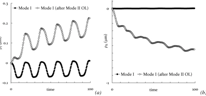
simulated, followed by 10 mode II cycles and 10 mode I cycles. The evolutions of ρ_II and ρ_I during the last 10 mode I cycles are plotted in Fig. 9 for the two cases.

(a) (b)

Figure 9: Simulations of crack tip plastic deformation for the loading cases used in the experiments

(Fig. 3). The black circles correspond to 10 mode I cycles after 160 mode I cycles. The empty circles correspond to 10 mode I cycles after 10 mode II overloads and 150 mode I cycles.

Calculated evolutions using the global mode (a) ρ_I, (b) ρ_II.

It is observed that, after the application of mode II overloads, the mode I plastic intensity factor range (Δ ) is increased by about a factor 2. If the crack growth rate is proportional to the plastic ρ_I intensity factor range, an increase of the fatigue crack growth rate after the application of the mode II overloads should be predicted using this model. This result is consistent with experimental observations. Furthermore, the mode I plastic intensity factor ρ_I increases progressively. Since this

model is incremental (ρ_I =Cst+

∫

dρ_I), the value of ρ_I alone is not significant. However, the

progressive increase of ρ_I should tend to blunt the crack and remove any crack closure effect.

4. Conclusions and prospects

The aim of this study was to establish a mixed-mode crack propagation model including history effects and to validate it using suitably chosen experiments. For this purpose, mixed mode fatigue

crack growth experiments were setup and showed that the studied material (a S355 NL steel used in marine applications) shows history effects in mixed mode fatigue crack growth. In the future it is planned to study in a systematic manner the fatigue crack growth resistance in this material under complex mixed-mode conditions.

Also, the first elements of a global mixed-mode plasticity model for the crack tip region were gathered. Since it is recognized that plasticity is at the origin of large history effects, a global cyclic elastic-plastic model for the crack tip region is useful for predicting mixed mode fatigue crack growth when variable amplitude conditions are encountered. This model is dedicated to be used in elastic analyses of cracked structures and should account for memory effects inherited from the non-linear behaviour of the material within the crack tip region. It can be used for instance in crack tip XFEM elements or in cohesive zones.

First, a multiscale approach was used to bring the results of detailed elastic plastic FE analyses from the local scale to the global scale. For this purpose, the velocity field in the crack tip region was approximated by the product of spatial reference fields, known a priori, and of their intensity factors. This approach is classical in LEFM. It was merely extended to the case of elastic-plastic

material behaviours by introducing two additional spatial reference fields ( c

I

u and c

II

u ) and their

intensity factors (ρ_I andρ_II) to account for plastic deformation within the crack tip region. Such an approximation was shown to be reasonably precise (less than 10% error), whatever the mode-mixity and the load history. Then during any loading history, the four intensity factor rates

(K&~ ,_II K&~ ,_I ρ& ,_II ρ& ) are determined by projecting the computed velocity field onto the basis of _I reference spatial fields that were constructed for all ( e

I u , e II u , c I u and c II u ).

In certain cases, approximating the velocity field by using only the “elastic” reference spatial

fields ( e II

u , u ) is just as precise as using the “enriched” approximation. In such cases, the crack tip e_I

region is considered as behaving elastically.

These FE results were used to define a global elastic plastic constitutive behaviour for the crack tip region. It includes: a yield criterion, a flow rule and a kinematic hardening evolution equation and sums up into a set of five scalar differential equations.

From the results of FE computations it was shown that an elastic domain can be defined for the crack tip region, which evolves during loading. This domain can be modelled by a yield criterion (generalization of the Von Mises criterion). During loading, the center of the yield locus moves

because of the growth of internal stresses. Therefore, two internal variables (K ,_IIX K ) were _IX

introduced to define the current position of this yield locus, and describe at the global scale these internal stresses. The normality flow rule was adopted for this problem and allows predicting ρ& _II and ρ& from the current state of the variables of the model and from the loading rate. And finally, _I the center of the yield locus moves along the plastic flow direction.

This model computes the evolutions of the current origin of the elastic domain for the crack tip region with good precision, compared with the FE method. The advantage is that the computations using this model, unlike FE computations, are very fast and efficient. The prediction of ρ& and _II ρ& _I remains to be improved, but the flow directions and the order of magnitude of the flow rate are correctly reproduced.

In the future, this model should be enriched. First, the evolution law of the crack closure as a function of ρ& and _II ρ& needs to be defined. Second, how the internal variables in this model evolve _I when the crack grows or deviates needs to be determined. This part can be done using the same approach, based on FE computations. Finally, a crack growth criterion, to predict the fatigue crack growth rate under general mixed mode non-proportional and variable amplitude loading conditions from the knowledge of ρ& and _II ρ& , needs to be developed. For this purpose fatigue crack growth _I experiments should be performed under complex loading conditions.

Acknowledgements

This work is supported by the French National Research Agency (ANR) through the project MIXMODFATFIS (No. BLAN06-1_134492) and by the Research Agency of the French Ministry of Defense (DGA).

References

1. Suresh, S., (1991), Fatigue of Materials, Cambridge University Press, Cambridge.

2. Mc Clung., R.C., (1996), proc. Fatigue 96, 6th International Fatigue Congress, Berlin

FRG, 6-10 May 1996.

4. Fleck, N.A., Newman, J.C., (1988) ASTM STP 982, pp. 319-341

5. Newman, J.C., (1981), ASTM STP 748, 1981, pp. 53-84

6. Schijve, J., (1973), Engineering Fracture Mechanics, (5) pp. 269-280.

7. McMillan, J.C., Pelloux, R.M.N., (1967), ASTM STP 415, pp. 505-532

8. Forman, R.G., Kearney, V.E. , Engle, R.M. (1967), Journal of basic Engineering, Vol 89,

pp. 459-64.

9. Pommier, S., (2002), Plane strain crack closure and cyclic hardening, Engineering

Fracture Mechanics, vol. 69, pp. 25-44.

10. Pommier, S., (2003), Cyclic plasticity and variable amplitude fatigue, International

Journal of Fatigue, vol. 25 pp. 983-997.

11. Pommier, S., (2006), proc. Plasticity'06 - 12th International Symposium on Plasticity and

its Current Applications. Halifax (Canada). 17-22 July 2006

12. Srinivas, V., Vasudevan, P., (1993), Study of the influence of mixed mode overload on

mode I fatigue crack propagation, Int J Vessels Piping, Vol. 56, pp. 409–417.

13. Gao, H., Upul, S.F. (1996), Effect of non-proportional overloading on fatigue life.

Fatigue Fract Eng Mater Struct, Vol. 19, pp. 1197–1206.

14. Dahlin, P., Olsson, M. (2008), Fatigue crack growth – Mode I cycles with periodic Mode

II loading, Int. J., Fatigue, Vol. 30, pp. 931-941.

15. Dahlin, P., Olsson, M. (2002), The effect of plasticity on incipient mixed mode fatigue

crack growth, Fat. Fract. Engng. Mat. Struct., Vol. 26, pp. 577-588.

16. Bold, P.E., Brown, M.W., Allen, R.J., (1992), A review of fatigue crack growth in steels

under mixed mode I and II loading. Fatigue Fract Eng Mater Struct, Vol. 15, pp. 965–977.

17. Wong, S.L., Bold, P.E., Brown M.W., Allen, R.J., (2000) Fatigue crack growth rates

under sequential mixed-mode I and II loading cycles. Fatigue Fract Eng Mater Struct, Vol. 23, pp.

667–674.

18. Nayeb-Hashemi, H., Taslim, M.E., (1987), Effects of the transient Mode II on the steady

state crack growth in Mode I, Eng Fract Mech, Vol. 26, pp. 789–807.

19. Doquet V., Bertolino G., (2008), Local approach to fatigue cracks bifurcation, Int. J.

Fat., Vol. 30 (5), pp. 942-950.

20. Doquet, V., Pommier, S., (2004), Fatigue crack growth under non-proportional mixed

mode loading in ferritic–pearlitic steel, Fatigue Fract Eng Mater Struct, Vol. 27, pp. 1051–1060.

21. Sander, M., Richard, H.A., (2006), Experimental and numerical investigations on the

influence of the loading direction on the fatigue crack growth, Int J. Fatigue, Vol. 28, pp. 583–591.

22. Sander, M., Richard, H.A., (2005), Finite element analysis of fatigue crack growth with

interspersed mode I and mixed mode overloads., Int J Fatigue, Vol. 27, pp. 905-913.

23. Erdogan, F., Sih, G.C., (1963), On the crack extension in plates under plane loading and

transverse shear, J Basic Eng, Vol. 85, pp. 519–525.

24. Qian, J., Fatemi, A., (1996) Mixed mode fatigue crack growth: A literature survey,

25. Pommier, S., Hamam R., (2007), Incremental model for fatigue crack growth based on a

displacement partitioning hypothesis of mode I elastic-plastic displacement fields, F Fatigue Fract

Eng Mater Struct, Vol. 30, pp. 582-598.

26. Hamam R., Pommier, S., Bumbieler, Fat., (2007), Variable amplitude fatigue crack

growth, experimental results and modelling, Vol. 29, Issue: 9-11, pp. 1634-1646

27. Pommier, S., Risbet M, (2005), Time-derivative equations for fatigue crack growth in

metals, Int. J. Fract., Vol. 131, pp. 79-106.

28. Li, C., (1989) Vector CTD criterion applied to mixed mode fatigue crack growth. Fatigue

Fracture Engng Mater. Structures, Vol. 12, pp. 59-65.

29. Lemaître, J., Chaboche, J.L., (2004), Mécanique des Matériaux Solides, Sciences Sup,

Dunod

30. Tada, H., Paris, P., (1973), The stress analysis of cracks handbook, Del research

corporation, Hellertown, Pennsylvania, USA

31. Pommier, S., Lopez-Crespo, P., Decreuse, P.Y., (2008) A multiscale approach to build a

global variational formulation of the mixed-mode cyclic elastic-plastic behaviour of the crack tip region, submitted to Fatigue Fract Eng Mater Struct