Handling the speed-accuracy trade-off in deep-learning based pedestrian detection systems

HAL Id: tel-02416418

https://tel.archives-ouvertes.fr/tel-02416418v2

HAL is a multi-disciplinary open access archive for the deposit and dissemination of sci-entific research documents, whether they are pub-lished or not. The documents may come from teaching and research institutions in France or abroad, or from public or private research centers.

L’archive ouverte pluridisciplinaire HAL, est destinée au dépôt et à la diffusion de documents scientifiques de niveau recherche, publiés ou non, émanant des établissements d’enseignement et de recherche français ou étrangers, des laboratoires publics ou privés.

based pedestrian detection systems

Ujjwal Ujjwal

To cite this version:

Ujjwal Ujjwal. Handling the speed-accuracy trade-off in deep-learning based pedestrian detection systems. Artificial Intelligence [cs.AI]. COMUE Université Côte d’Azur (2015 - 2019), 2019. English. �NNT : 2019AZUR4087�. �tel-02416418v2�

Gestion du compromis

vitesse-précision dans les systèmes de

détection de piétons basés sur

apprentissage profond

Ujjwal

INRIA Sophia Antipolis, STARS

du grade de docteur en Automatique, Traitement du Signal et des Images

d’Université Côte d’Azur

Dirigée par : François Brémond Co-encadrée par : Aziz Dziri Soutenue le : Novembre 13, 2019

Devant le jury, composé de : Président du jury :

Frédéric PRECIOSO, Professeur, Université

Côte d’Azur

Rapporteurs :

Christian WOLF,Maître de conférences

, HDR,

INSA de Lyon

Alexandre Alahi, Professeur assistant tenure track, EPFL

Thierry Chateau, Professeur, Université Clermont-Auvergne

THÈSE DE DOCTORAT

Ujjwal

Directeur de thèse: François Bremond STARS, Inria Sophia Antipolis, France

RÉSUMÉ

L’objectif principal de cette thèse est d’améliorer la précision des systèmes de détection de piétons à partir d’image, basés sur l’apprentissage profond sans sacrifier à la vitesse de détection. Pour ce faire, nous effectuons d’abord une analyse quantitative systématique des diverses techniques de détection de piétons à partir d’image. Cette analyse nous permet d’identifier les configurations optimales des différentes composantes d’un système de détection de piétons. Nous examinons ensuite la question de la sélection des meilleures couches convolutionnelles pour extraire les caractéristiques visuelles pour la détection des piétons et proposons un système appelé Multiple-RPN, qui combine plusieurs couches convolutives simultanément. Nous proposons le système Multiple-RPN en deux configurations - une fusion-tôt et une fusion-tardive; nous démon-trons ensuite que la fusion-tôt est la plus performante, en particulier pour la détection de piétons de petites tailles et les cas d’occultation de piétons. Cette étude fournit aussi une évaluation quantitative de la sélection des couches convolutionnelles. Nous intégrons ensuite l’approche de la fusion-tôt avec une étape de segmentation pseudo-sémantique pour réduire le cout de traitement. Dans cette approche, la segmentation pseudo-sémantique permet de réduire les faux positifs et les faux négatifs. Ceci, associé à un nombre réduit d’opérations, permet d’améliorer simultanément les performances de détection et la vitesse de traitement ( 20 images/seconde) ; les pe.fo

rmances sont compétitives avec celles de l’état de l’art sur les bases de données caltech-raisonable (3.79% de taux d’erreurs) et citypersons (7.19% de taux d’erreurs). La dernière contribution de cette thèse est la proposition d’une couche de classification des détections potentielles, qui réduit encore le nombre d’opérations de détection. Il en résulte une réduction de la vitesse de détection ( 40 images/seconde) avec une perte minime de performance de détection (3.99% et 8.12% de taux d’erreurs dans les bases de donnéealtech-raisonable et citypersons respectivement) ce qui reste compétitif avec l’état de l’art.

by

Ujjwal

Supervisor: François Bremond STARS, Inria Sophia Antipolis, France

ABSTRACT

The main objective of this thesis is to improve the detection performance of deep learning based pedestrian detection systems without sacrificing detection speed. Detection speed and accu-racy are traditionally known to be at trade-off with one another. Thus, this thesis aims to handle this trade-off in a way that amounts to faster and better pedestrian detection. To achieve this, we first conduct a systematic quantitative analysis of various deep learning techniques with respect to pedestrian detection. This analysis allows us to identify the optimal configuration of various deep learning components of a pedestrian detection pipeline. We then consider the important question of convolutional layer selection for pedestrian detection and propose a pedestrian detection sys-tem called Multiple-RPN, which utilizes multiple convolutional layers simultaneously. We propose Multiple-RPN in two configurations – early-fused and late-fused; and go on to demonstrate that early fusion is a better approach than late fusion for detection across scales and occlusion levels of pedestrians. This work furthermore, provides a quantitative demonstration of the selectivity of various convolutional layers to pedestrian scale and occlusion levels. We next, integrate the early fusion approach with that of pseudo-semantic segmentation to reduce the number of processing operations. In this approach, pseudo-semantic segmentation is shown to reduce false positives and false negatives. This coupled with reduced number of processing operations results in improved detection performance and speed ( 20 fps) simultaneously; performing at state-of-art level on caltech-reasonable (3.79% miss-rate) and citypersons (7.19% miss-rate) datasets. The final con-tribution in this thesis is that of an anchor classification layer, which further reduces the number of processing operations for detection. The result is doubling of detection speed ( 40 fps) with a minimal loss in detection performance (3.79% and 8.12% miss-rate in caltech-reasonable and citypersons datasets respectively) which is still at the state-of-art standard.

Résumé i

Abstract iii

Dedications v

1 Introduction 1

1.1 Pedestrian Detection . . . 1

1.2 Pedestrian Detection as a Machine Learning Problem . . . 2

1.3 A Linguistic Clarification of the term “Pedestrian” . . . 5

1.4 Challenges in Deep Learning based Pedestrian Detection . . . 6

1.5 Contributions of the Thesis . . . 8

2 Pedestrian Detection Approaches in Deep Learning 15 2.1 Introduction . . . 16

2.2 Detection Systems – Single-Stage and Two-Stage . . . 16

2.2.1 Two-stage detectors . . . 18

2.2.2 One-Stage detectors . . . 22

2.3 Pedestrian detectors as extensions of general-category detectors . . . 24

2.3.1 Architectural Refinements . . . 26 2.3.2 Loss Function . . . 28 2.3.3 Classifier Selection . . . 30 2.3.4 Semantic Segmentation . . . 30 2.3.5 Boosting . . . 31 2.4 Datasets . . . 32

2.4.1 Caltech Pedestrian Dataset. . . 32

2.4.2 CityPersons . . . 33

2.4.3 BDD100K . . . 33

2.5 Evaluation Metrics . . . 34

2.6 Conclusions . . . 34

3 Quantitative Analysis of Pedestrian Detection in Deep Learning 37 3.1 Introduction . . . 37

3.2 Related Work . . . 39

3.3 Common Experimental Settings . . . 40

3.3.2 Learning Rate Schedule and Momentum . . . 41

3.3.3 Initializer . . . 42

3.4 Evaluation Protocols . . . 42

3.5 Analysis of Design Choices for Pedestrian Detection . . . 42

3.5.1 Base Network Architecture. . . 42

3.5.2 Convolution Techniques . . . 47

3.5.3 Role of Convolutional Layer Selection in Pedestrian Detection . . . . 50

3.5.4 Anchor Parameters . . . 51

3.5.5 Loss Function . . . 53

3.5.6 Role of Dataset Resolution in Pedestrian Detection . . . 54

3.6 What is the best pedestrian detector . . . 55

3.6.1 Base Network Architecture . . . 55

3.6.2 Feature Map Resolution . . . 56

3.6.3 Anchor Design . . . 56

3.6.4 Semantic Features . . . 57

3.6.5 Classifier Selection . . . 57

3.6.6 Post-Processing . . . 57

3.7 Conclusion . . . 58

4 A Multiple layer RPN approach to Pedestrian Detection 61 4.1 Introduction. . . 62

4.2 Hierarchical nature of CNN features . . . 62

4.3 Datasets and Evaluation Metrics. . . 64

4.3.1 Datasets . . . 64

4.3.2 Evaluation Metrics . . . 64

4.4 Layer-wise analysis of CNN layers’ effect on scale and occlusion . . . 64

4.4.1 Effect of CNN layers on scale and occlusion based detection . . . 66

4.4.2 Pedestrian Detection System Design . . . 67

4.5 Experiments and Results . . . 71

4.5.1 Training . . . 71

4.5.2 Results. . . 71

4.6 Analysis . . . 73

5 A Spatial Attention Approach to Pedestrian Detection 75 5.1 Introduction. . . 76

5.2 Revisiting the Speed/Accuracy Tradeoff. . . 76

5.3 Related Work . . . 77

5.4 Fundamental traits of single-stage and two-stage detectors . . . 79

5.4.1 Two-stage detectors . . . 79

5.4.2 One-stage detectors . . . 80

5.5 On the number of processing targets for convolutional detectors . . . 80

5.6 Reducing the Number of Processing Targets . . . 82

5.7 On Semantic Segmentation to Reduce Processing Targets . . . 83

5.8 Proposed Pipeline for Fast Pedestrian Detection . . . 85

5.8.1 Input . . . 86

5.8.3 Deformable Convolution . . . 88

5.8.4 Semantic Fully Convolutional Layer. . . 90

5.8.5 Anchor Location Selection . . . 91

5.8.6 Classification and Bounding Box Regression . . . 92

5.9 Training . . . 93

5.9.1 Loss Function . . . 93

5.9.2 Implementation Details . . . 94

5.10 Experiments and Results . . . 95

5.10.1 Datasets . . . 95

5.10.2 Results. . . 95

5.10.3 Ablation Studies . . . 97

5.10.4 Spatial Attention : Comparison with RPN . . . 98

5.11 Discussion and Conclusions . . . 98

6 Reducing anchors even more : Faster and Better 101 6.1 Introduction . . . 101

6.2 Related Work . . . 102

6.3 Performance Characteristics . . . 103

6.3.1 Deformable Convolutional Layer . . . 103

6.3.2 Concatenation of pedestrian probability map and deformable con-volution output . . . 106

6.3.3 Two-Step classification and regression . . . 107

6.3.4 Input Size . . . 107

6.4 Proposed Approach . . . 108

6.4.1 Summary . . . 108

6.4.2 Anchor Selection Layer. . . 108

6.5 Training and Implementation Details . . . 111

6.5.1 Loss Function . . . 111

6.6 Experiments, Results and Analysis. . . 112

6.6.1 Datasets . . . 112

6.6.2 Hyperparameter settings . . . 112

6.6.3 Results and Analysis . . . 113

6.7 Ablation Studies . . . 114

6.7.1 Comparison with Region Proposal Network . . . 114

6.7.2 Impact of anchor selection layer. . . 114

6.8 Conclusions . . . 115

7 Conclusion and Future Work 117

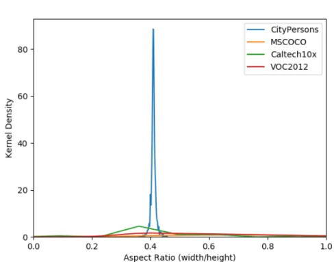
1.1 A plot of aspect ratio (width/height) distribution of “pedestrians” in 4 different datasets –2 general-category (MSCOCO and Pascal VOC) and 2 pedestrian-specific (CityPersons and Caltech10x). It can be seen that while there is a clear peak in the distribution for pedestrian datasets, the distri-bution for general-category datasets is relatively uniform. . . 3

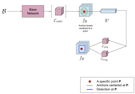
1.2 General pipeline of an anchor based object or pedestrian detection system. . 9

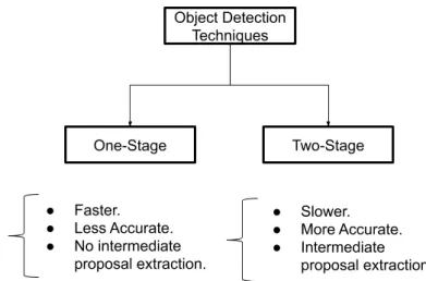
2.1 Major characteristics of one-stage and two-stage object detectors. . . 18

2.2 Feature handling mechanism of Faster-RCNN and other two-stage detectors. 19

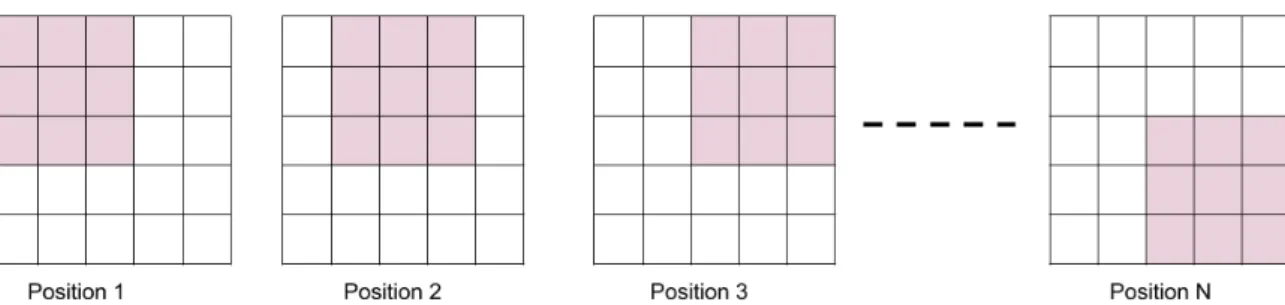
2.3 (Top):- Different positions of a convolutional kernel sliding over a feature

map. (Bottom):- The location of a filter kernel for 4 confocal anchors. The

dark red pixel is a specific location on the feature map. The pink region depicts the convolutional kernel. The unfilled dark red rectangles are the anchors. Since for each of the 4 confocal anchors, the location of the filter kernel is fixed, the convolutional output value is the same and for all 4 confocal anchors. . . 20

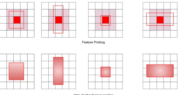
2.4 Intra anchor feature pooling vis-à-vis feature probing. Top: Feature probing

at a feature map location indicated by a dark red pixel. The pink region shows a 3 × 3 kernel at the location, while the unfilled dark red rectangles are the anchors centered at that location. Each of those anchors share the same feature vector vvv. vvv is the result of convolution of the kernel with the feature map at the feature map location. Bottom: Intra-anchor feature

pooling for the same scenario as inTop. Each anchor has a different feature

vector, which is obtained by extracting features from inside the anchor and then using ROI-Pooling [130], ROI-Align [63] or resizing [23] followed by flattening. It is evident that intra-anchor feature pooling produces more anchor-specific features. . . 21

2.5 Difference between ROI-Pooling [130] and ROI-Align [63] mechanisms for intra-anchor feature pooling . . . 23

2.6 Feature handling mechanism of one-stage detectors. . . 24

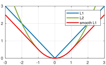
2.7 A comparison of L1, L2 and smooth-L1 loss functions.. . . 29

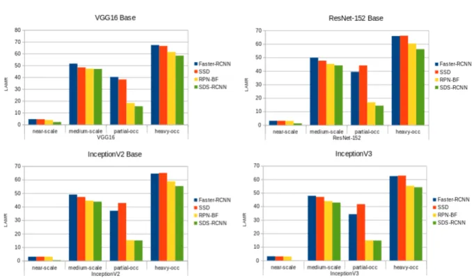
3.1 Scale-wise bar charts with a visual summary of figures in tables 3.1 through 3.4. . . 45

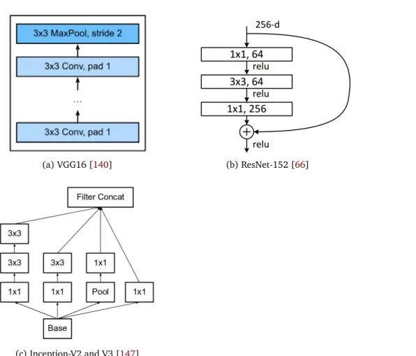
3.2 Building blocks of CNN architectures used in our analysis of the impact of base network on pedestrian detection performance. . . 46

4.1 Visualization of feature maps from two different layers in VGG-16 network trained on ILSVRC-2012 dataset. . . 63

4.2 Block Diagram of the proposed pedestrian detection system. The data flow for the study in section 4.4, is indicated using dashed green lines. We later improve upon this and the final system’s data flow is shown in solid black arrows. The red dashed lines in the diagram refer to the location of pooling layers in VGG16 [140], where the feature map changes size. . . 65

4.3 The proposed pedestrian detection system with early fusion. . . 70

5.1 Impact of number of RPN proposals on the recall of pedestrians. Shown for 4 techniques. Of these except RPN [177], the others are non-deep learn-ing based techniques. As the number of proposals is increased, the recall is stablized over a large range of intersection-over-union with groundtruth bounding boxes. The dataset used here is the caltech-reasonable test set. . . 81

5.2 Top 35 proposals (green) generated by RPN [130] for an image in the caltech-reasonable test set. The red boxes correspond to groundtruth

bounding boxes for the labelled pedestrians. . . 84

5.3 Left : An image with pedestrian bounding boxes. Right : The pseudo

segmentation mask for the image on the left. . . 85

5.4 Pixelwise classification probability of image regions to be pedestrian. . . 86

5.5 Block diagram of the proposed approach.. . . 87

5.6 Architectural details of various members of the ResNet family. Courtesy of [67]. . . 88

5.7 Standard convolution process in CNNs. The convolutional kernel computes correlation with feature map values for every sliding location. The correla-tion result becomes the feature map value for the center point locacorrela-tion of the filter in the output feature map. . . 89

5.8 a: The sliding location of the filter kernel, b,c and d: Various examples of

possible offset locations. The offsets are applied to each location at the slid-ing position of the kernel. The correlation is computed between the filter kernel and the feature map values at the locations after applying offsets (in blue). . . 89

5.9 Normal Convolution . . . 90

5.10 Deformable Convolution . . . 90

5.11 Sampling locations shown for one pedestrian with a): Normal Convolu-tion and b): Deformable ConvoluConvolu-tion. In both cases the convoluConvolu-tion

ker-nel is 3 × 3 with stride 1. . . 90

5.12 Semantic Segmantation module of the proposed system. . . 91

5.13 Some detections (Left) on the validation set of caltech-1x dataset compared

with corresponding groundtruth (Right).. . . 96

6.1 Block diagram of the approach proposed in chapter 5. Reproduced here for simplicity and comparison with the approach presented here in figure 6.2 . . 104

6.2 Block diagram of the proposed approach. This block diagram differs from figure 6.1 in terms of many refinements which allow for better inference without loosing detection accuracy. . . 105

6.3 Illustration of offset calculation for a 3 × 3 deformable convolution operation.106

6.4 An occluded pedestrian with full-body bounding box (green) and visible

bounding box (blue). Red anchors are confocal with the magenta anchor.

The red anchors do not overlap well with both the full-body and visible

bounding box, while themagenta anchor has sufficient overlap with both. . 109

6.5 The anchor selection layer. For illustration it is assumed that all anchors have been generated by a base anchor of size 64 × 64 and have an aspect ratio of 0.41 (width/height). The anchor at scale 1 then corresponds to a box of size ∼ 100 × 41. For a feature stride of 16, a kernel of size 7 × 3 will cover the corresponding area of this box in the feature map. For other scale values, the kernel size can be similarly defined. . . 110

2.1 A brief summary of some popular deep learning approaches to pedestrian detection. . . 25

2.2 Enhancements introduced by some contemporary pedestrian detection sys-tems. . . 26

2.3 A summary of 3 public datasets used in our work. . . 32

3.1 Relative performance of different techniques on caltech pedestrian dataset with VGG16 as base network. Reasonable subset is described in chapter

2. For scale analysis, only unoccluded pedestrians are used. For occlusion, only pedestrians with heights H ≥ 50 pixels are used. For Near-scale, H ≥ 80 pixels. For Medium-scale, H ∈ [30, 80] pixels. Partial-occ refers

to occlusionO ∈ [1, 35]%. Heavy-occ refers to occlusion O ∈ [35, 80]%. All

figures are LAMR percentage values.The best result in each column is in bold. . . . 43

3.2 Relative performance of different techniques on caltech pedestrian dataset with ResNet-152 as base network. Column description same as in table 3.1. All figures are LAMR percentage values. The best result in each column is in bold. . . . 43

3.3 Relative performance of different techniques on caltech pedestrian dataset with InceptionV2 as base network. Column description same as in table 3.1. All figures are LAMR percentage values. The best result in each column is in bold. . . . 44

3.4 Relative performance of different techniques on caltech pedestrian dataset with InceptionV3 as base network. Column description same as in table 3.1. All figures are LAMR percentage values. The best result in each column is in bold. . . . 44

3.5 Impact of Depthwise Separable convolution (w) when replacing normal

convolutional layer (w/o) in the last CNN layer in 4 pedestrian detection

frameworks. . . 49

3.6 Impact of Depthwise Separable convolution (w) when replacing normal

convolutional layer (w/o) in the last CNN layer in Faster-RCNN with VGG16

as the base architecture. . . 49

3.7 Impact of anchor aspect ratio on Miss-Rate performance on caltech dataset with InceptionV2 as base network. . . 52

3.8 Effect of anchor scales on miss-rate performance on caltech-reasonable dataset. The base anchor size is 128 × 128. The base network is Incep-tionV2. The aspect ratio of anchors is 0.41. . . 52

3.9 Impact of focal loss inclusion in the loss functions of Faster-RCNN and SSD. We choose α = 0.5 and γ = 2 as in [98]. Anchor parameters are chosen as delivering best results according to tables 3.7 and 3.8. InceptionV2 is the base network. . . 54

3.10 Impact of repulsion loss inclusion in the loss function of Faster-RCNN. An-chor parameters are chosen as delivering best results according to tables 3.7 and 3.8. InceptionV2 is the base network. . . 54

3.11 Impact of relative ordering of datasets of different resolutions when doing training and fine-tuning. It is better to first train a dataset with a high-resolution dataset and then fine-tuning it with a low high-resolution dataset. Caltech refers to caltech reasonable. BDD100K refers to pedestrians with heights> 50px. All figures are LAMR values . . . 55

4.1 Log-Averaged miss rate for pedestrians of different heights by different lay-ers in Caltech-reasonable (test) dataset. . . . 66

4.2 Log-Averaged miss rate for varying occlusion levels by different layers in Caltech-complete (test) dataset. For the Caltech-complete we have used the old annotations (pedestrian height > 50 pixels.). . . 67

4.3 Anchor scales chosen for different layers. The notation [A,B,C] in the sec-ond column refers to minimum scale as A, maximum scale as B with a step-size of C (all in pixels). . . 68

4.4 Log-averaged miss rate over different subsets of caltech[46]. The testing and training subsets are shown in the 3rd _{and 4}th _{columns. New caltech}

annotations of [46] are used for training and testing. . . 71

4.5 Comparison with other works with performance on Caltech-reasonable(test set) of caltech1x . . . 71

4.6 Miss-Rates for different pedestrian height ranges in the caltech-all testing (1x-test) set. This includes all occlusion levels. New annotations from [46] are used for training and testing. . . 72

5.1 A comparison of the number of processing targets for Faster-RCNN [130] and SSD [102] with VGG16 [140] as the base network. For Faster-RCNN the figures correspond to 600 object proposals being selected for processing by the second stage. For SSD, the number of processing targets correspond to the network topology as shown in [102]. . . 82

5.2 Performance of the proposed approach on caltech1x and citypersons-validation set. (|C| = 350). . . 94

5.3 Comparative performance of the proposed approach with other pedestrian detectors. . . 94

5.4 Summary of ablation studies on caltech-1x dataset. These ablations were performed for |C| = 350 and directly training the system on caltech10x-train. 95

5.5 Comparative performance of the inference speed of various detectors. For our proposed detector, the inference speed corresponds to |C| = 350. . . 96

5.6 Effect of varying the hyper-parameter |C|. The miss-rate for caltech-1x is based on model pre-trained on citypersons-train followed by fine-tuning on caltech-1x. The miss-rate for citypersons-val is based on model trained on citypersons-train. . . 97

5.7 Impact of varying the hyper-parameter |C| on inference speed.. . . 97

5.8 Comparison between spatial attention and RPN on the basis of LAMR . . . . 98

6.1 Intersection-over-union analysis of the performance of semantic segmenta-tion module. . . 107

6.2 LAMR of our proposed approach over caltech-reasonable and cityper-sons(val) datasets. Our best results on caltech-reasonable (test) are achieved through pre-training on citypersons(train) dataset. . . 111

6.3 Summary of dataset size of caltech-reasonable [34] and citypersons [179] dataset. . . 112

6.4 Performance comparison of the proposed method with other methods for caltech-reasonable test set and citypersons validation set. The speed figures are in frames per second. . . . 112

6.5 Ablation study of RPN vs. our approach using semantic segmentation and anchor selection layer on the citypersons(validation) dataset. . . 114

Introduction

Contents

2.1 Introduction . . . 16

2.2 Detection Systems – Single-Stage and Two-Stage . . . 16 2.2.1 Two-stage detectors . . . 18

2.2.2 One-Stage detectors . . . 22

2.3 Pedestrian detectors as extensions of general-category detectors . . . 24 2.3.1 Architectural Refinements . . . 26 2.3.2 Loss Function . . . 28 2.3.3 Classifier Selection . . . 30 2.3.4 Semantic Segmentation . . . 30 2.3.5 Boosting. . . 31 2.4 Datasets . . . 32 2.4.1 Caltech Pedestrian Dataset. . . 32

2.4.2 CityPersons . . . 33

2.4.3 BDD100K . . . 33

2.5 Evaluation Metrics . . . 34

2.6 Conclusions. . . 34

1.1

Pedestrian Detection

Pedestrian detection refers to the determination of regions in an image (or in individual

frames of a video stream), such that each determined region contains one pedestrian. As

such, it is a specific instance of the more general problem of object detection in computer vision – i.e limited only to pedestrians. Pedestrian detection is usually studied as a separate problem owing to its several applications which were recognized quite early on – e.g.

video surveillance, person tracking and autonomous driving. Earliest works on pedestrian

application domains. In the aforementioned applications like autonomous driving and

video surveillance, the performance of a pedestrian detection system has a major cost factor

in terms of safety concerns. For instance, failure of an autonomous driving system to detect a pedestrian crossing a street can result in mishaps with a potential to damage human life. Since late 1980’s, when the first experiments with prototypes for autonomous vehicles [151] and automated video surveillance [62,121] were carried out, these applications have entered mainstream usage on a large scale. This has led to a corresponding escalation in the safety concerns associated with the performance of pedestrian detection systems [78]. The large-scale adoption of these systems is expected to steadily increase in the future [59,26]. In [27], it is reported that in real-life scenarios, contemporary detectors’ ability to detect pedestrians in advance of fatal collisions vary from < 30% to > 90% of fatalities. This range needs to be bridged towards lower values to ensure the feasibility of self-driving cars in real-life scenarios on a large-scale. Thus despite being worked upon since 1980’s, pedestrian detection is still a relevant problem and plays a key role in ensuring the safety of modern applications such as autonomous driving.

From the previous discussion we gather that, in real-life pedestrian detection systems, simply detecting pedestrians is not important on its own; it has to be coupled with the ability to detect pedestrians well in advance. The fundamental objective of this thesis is to jointly address these coupled problems of detection accuracy and detection speed; a fundamental practical problem in autonomous vehicles. From a technical perspective, pedestrian detection and its parent problem of object detection are formulated as machine learning problems. In the next section, we understand the nature of pedestrian detection as a machine learning problem. This renders greater clarity to our understanding of the technical challenges of pedestrian detection and hence recognizing the technical areas of our contribution.

1.2

Pedestrian Detection as a Machine Learning Problem

Pedestrian detection is a localization problem. This means that a pedestrian detection system needs to delineate locations in an image with pedestrians by drawing a rectangular bounding box around the pedestrians This localization problem in machine learning terms is a union of two problems – a) A two-class classification problem where every image-region must be classified for the presence or absence of a pedestrian and, b) A regression problem where given a set of features representing an image region, estimation of the 4 corner coordinates of the rectangle bounding a pedestrian at that location; if one exists; must be made.

This is an appropriate stage to point out some technical differences between pedes-trian detection and its parent problem of object detection. Firstly, object detection is a

Figure 1.1: A plot of aspect ratio (width/height) distribution of “pedestrians” in 4 dif-ferent datasets –2 general-category (MSCOCO and Pascal VOC) and 2 pedestrian-specific (CityPersons and Caltech10x). It can be seen that while there is a clear peak in the distri-bution for pedestrian datasets, the distridistri-bution for general-category datasets is relatively uniform.

localization problem involving C + 1 classes, where C refers to different classes of ob-jects (an addition of 1 is made to reflect the background class, that is image regions which

correspond to no object of interest among C classes). In contrast, pedestrian detection is

a 2 class problem. Secondly, pedestrians have a relatively rigid orientation (e.g:- upright

pose and small deformation due to walking stance), while in general-category datasets like

MSCOCO [99] and Pascal VOC [48], object categories exhibit a wider range of poses and deformation. This is illustrated in figure1.1, where it can be seen that the aspect ratio dis-tribution of bounding boxes for pedestrians bears a major similarity amongst pedestrian detection datasets and differs significantly from that in general object category datasets. Pedestrian detection techniques have evolved to put special emphasis on these characteris-tics (e.g.- techniques such as SDS-RCNN [14] and RPN-BF [177] utilize the mode of aspect ratio distribution of pedestrians to demonstrate improved performance). This trend is not observed in general category object detection systems.

As in any machine learning problem in computer vision, the quality of features ex-tracted from images is of quintessential relevance in pedestrian detection. Most of the

early pedestrian detection systems [31,50] were dependent on manually specified func-tions for feature extraction. For example the histogram of oriented gradients (HoG) feature [31] can be modelled by a nonlinear function which computes gradients, divides its in-put into grids and performs binning of gradients in each cell of a grid. The parameters of this function (e.g:- number of orientations, number of cells etc) has to be set manually and cannot not be learnt during the training process automatically. While these parame-ters can be tuned for specific datasets through thorough experimentation, it is difficult to tune them to perform well across different datasets. With the advent of deep learning in computer vision, the trend has shifted towards utilizing a deep neural network (DNN) for feature extraction. This is on account of the fact, that DNNs are trainable as against man-ually specified functions whose parameters were generally non-trainable. This facilitates the learning of task-specific features by DNNs, thereby leading to better performance by DNNs in nearly all domains of computer vision including pedestrian detection. Follow-ing this observation, we limit ourselves to deep learnFollow-ing based pedestrian detection systems in this thesis.

At this point one can be described, the essential basic differences between the mul-titude of deep learning based pedestrian systems. Understanding these key differences is the key to understand the contemporary challenges in pedestrian detection followed by the outline of technical contributions presented in this thesis. We enumerate these essential differences below :

1. Selection of DNN : Many classes of DNNs are known today – restricted boltzmann

machines (RBMs), convolutional neural networks (CNNs) and recurrent neural net-works (RNNs) to name a few. Within each of the above classes, there are many

variations available. Pedestrian detection techniques utilizing multiple such vari-ations of DNNs are known today [14, 159, 105]. Different DNNs extract varying features dependent upon their topology and the task-at-hand. Hence, this is one of the prominent differences found amongst pedestrian detection systems.

When processing static RGB images, CNNs are the most commonly used DNNs owing to their suitability in representing static spatial inputs. RNNs are difficult to use with images because of the absence of a unique sequential structure in images (due to their 2D structure). Even if, a convention is adopted (such as raster sequencing), another problem related to the memory problem in RNNs [132]. Processing a large image by modelling it as a sequence of pixels, results in a long RNN, which makes learning difficult due to the vanishing gradient problem [132]. Natural images are highly varying in appearance and this makes it difficult for RBMs to model the joint probability density of images. Due to these reasons, in this thesis, we exclusively work with CNNs for pedestrian detection.

2. Training and Fine-tuning Strategy : The training of DNNs determines the nature of features extracted by them. This training is an optimization task guided by an objective function, more commonly known as a loss function. This is one of the most significant ways in which different pedestrian detection techniques differ, thereby being one of the most important technical differences amongst pedestrian detection systems.

A previously trained DNN, can be retrained on a different dataset with a different loss function, taking its previously trained (or pre-trained) state as the initialization point for optimization. This process is known as fine-tuning the DNN. Fine-tuning is known to lead to faster training and better results [136,149] and hence is widely practised in deep learning. For fine-tuning, various strategies are significant such as selection of the pre-trained state (i.e dataset on which pre-training was done) [179,

85] and fine-tuning only specific layers while leaving other layers fixed to the pre-trained state [76, 87]. Thus, when training or fine-tuning a DNN for pedestrian detection, the specifics of training and fine-tuning strategies play a crucial role. 3. Feature Utilization : Features are extracted by DNNs for an entire image. For

the purpose of localization, features corresponding to different image regions are then utilized. This is known as a feature handling mechanism. This is one of the most important technical differences amongst pedestrian detection systems, since this mechanism has a direct impact on the quality of final detections.

4. Post-Processing Approaches : The detections obtained from a DNN usually encap-sulate multiple detections of the same pedestrian and have to be post-processed to eliminate duplicate detections. There are many classes of post-processing techniques such as non-maximal-suppression (NMS) and depending upon their usage, the qual-ity of detections can vary, thereby forming it as an important point of difference amongst pedestrian detection systems.

Having outlined a global outlook of the technical subtleties of pedestrian detection as a machine learning problem, we now embark upon a description of the technical challenges in pedestrian detection. However, we take a brief detour and settle the choice of the nomenclature “pedestrian”.

1.3

A Linguistic Clarification of the term “Pedestrian”

The exact nature of the term “pedestrian” in our work needs some elaboration. This is owing to the following reason.

Annotation protocols followed for creating different public datasets for pedestrian de-tection are different. For instance, in the caltech pedestrian dataset [33] and the BDD100K dataset [174], bounding boxes around instances such as people riding a bicycle are anno-tated as pedestrians. On the other hand, the citypersons dataset [179], there are separate annotations for person and rider. In most applications, such as autonomous driving, all humans need to be detected. Thus, the exact interpretation of “pedestrians” is dataset-specific.

In this thesis, we consider all annotations of humans as “pedestrians”. This as-sumption frees us from fine-grained specifics of different annotation protocols, while also ensuring focus on detecting humans.

1.4

Challenges in Deep Learning based Pedestrian Detection

Scale : Detection of small-scale pedestrians is a major challenge; scale referring to the height (H) of a pedestrian. For instance, in the complete caltch pedestrian dataset [33], the detection quality for pedestrians with H < 80 pixels is ∼ 40% lower than that for H > 80pixels [183]. Pedestrian appearance varies significantly between large and small scales. For instance, small-scale pedestrians are mainly delineated by their contour, while large-scale pedestrians have more elaborate appearance with facial and body details. As a result, it is difficult to distinguish small-scale pedestrians with background clutter

(e.g:-trees). Technically, the challenge is in learning features which decompose small-scale

pedestrians and background entities into 2 distinct clusters in the feature space; despite their similar appearance in the image space. CNNs employ spatial pooling between a sub-set of layers, thereby increasing the feature stride down the network. As a result, the information of small-scale pedestrians gets restricted to a very small set of feature map pixels. In contemporary detectors [130, 102], feature map regions are represented by a fixed length feature vector for classification and regression. The construction of this vector takes place through non-linear operations such as ROI-pooling [130] or opera-tions resulting in interpolation errors [23]. This leads to a less reliable feature represent-ing small-scale entities. In deep learnrepresent-ing, scale has received significant attention in both general-category [142] and pedestrian-specific techniques [183,16] with an objective to build scale-invariant systems. However despite several approaches such as upsampling of

recently proposed method of scale normalization [142], there stands a significant gap to be bridged.

Occlusion : A highly occluded pedestrian is difficult to detect. As in the case of scale, the detection quality in the complete caltech dataset degrades with increasing occlusion levels [183]. Depending upon the entity occluding a pedestrian and the contemporary pose of the pedestrian, occlusion can arise in a wide range of configurations. Some datasets such as caltech [33] and citypersons [179] come with with groundtruth bounding box annota-tions encompassing both visible and full-body regions of pedestrians. However, especially in the case of higher occlusion levels, the visible bounding box can be particularly small and results in the same challenges as scale. Given a feature representing a region con-taining a pedestrian, it is interesting to reliably decompose it into two separate feature representations – one representing the visible pedestrian part and the other representing the region occluding the pedestrian. This approach, often known as feature disentangle-ment [155] is recent and popular, but has been applied to a select few problems such as face recognition and pose estimation; both of which are non-localization problems.

Illumination variations and other Environmental Factors : Under low illumination conditions, detecting pedestrians is particularly difficult. Low illumination conditions rob off most of the information about edges and other basic low-level features from an im-age. These low-level features are usually detected by the early CNN layers [86,176], and form the basis for feature decomposition by later layers. The lack of these features under low illumination, changes the statistical properties of the input to a CNN. In addition, un-der low-level illumination, other features such as image-noise become more prominent, which further cause degradation of performance. Most existing public datasets are lim-ited to daytime environment, where illumination variations are relatively milder. Lack of any corresponding training data makes it difficult to train or tune a system to low illumi-nation conditions. Other environmental factors such as weather, in a similar way cause degradation of performance.

Cross dataset generalization : Generalization performance of a machine learning sys-tem is a well known and fundamental problem. Generalization performance analysis of a machine learning system involves studying its test-time performance on various datasets, which can be potentially different from the dataset(s) used for training it. The source of this issue of cross-dataset generalization lies in the distribution function modelling a dataset. A machine learning problem is computing a mapping F : X −→ Y, where the do-main X represents the input data and the co-dodo-main Y represents the target (classification

or regression). Each x ∈ X can be thought to be a random variable generated by a

prob-ability distribution function P. During training pre-specified x ∈ X and y ∈ Y are used to model F . For different datasets, P could be different, thereby essentially changing the domain of F . Thus F modeled during training might not fit a dataset with a different P. This phenomenon is also known as dataset bias [154]. The most common approach to mit-igate this phenomenon is to map the data to a different space R modeled by a distribution function PR, such that P and PRgenerate independent random variables. Deep learning

has proved to be more successful than handcrafted feature-based techniques in ensuring better cross-dataset generalization; though far from perfect. Fine-tuning a deep learning based pedestrian detection model on a new dataset (from the same problem domain) is of-ten found to have better performance than the original model. However, fine-tuning is an impractical technique when taken to real-world applications such as autonomuos driving, where a system has to respond favorably in potentially unseen pedestrian instances. These unseen instances may differ in scale, appearance or weather conditions as described be-fore. This makes it pertinent to analyze pedestrian detection systems from the perspective of cross-dataset performance.

1.5

Contributions of the Thesis

First we give a broad outline of the problem areas we have addressed in this thesis. We then follow-up with a summary of different chapters in this thesis in terms of their content and contributions.

To facilitate the outline of our focus areas, we refer to figure1.2showing the general pipeline of a deep learning based object or pedestrian detection system. The input image is first processed by a CNN to obtain a feature map. This is followed by a “region selection

strategy” which selects a set of locations in the feature map for further processing. Some

detection systems process all possible locations in the feature map. In general, the region selection strategy can be encapsulated as a transformation which takes as input a feature map and outputs a set of locations or regions inside the feature map which are processed further. More details on this can be found in chapter2. Given a location or region inside a feature map, it is represented by a feature vector. The exact representation of a region us-ing a feature vector varies from one method to other and the correspondus-ing mechanism is known as the “feature handling mechanism” (described in detail in chapter2). The feature vector representing a region is then classified and regressed. If classified as a pedestrian, the bounding box obtained from the regression represents the bounding box coordinate of the pedestrian.

From the above description emerges 3 important perspectives which we address in this thesis.

1. Training and Fine-tuning strategy : Training and fine-tuning of deep CNNs is a non-trivial task involving non-linear optimization which is heavily influenced by the selection of various hyperparameters and optimization techniques. In addition, var-ious pedestrian detection techniques share some common elements such as anchors which invoke additional hyperaparameters. Another interesting observation is the selection and ordering of datasets used for training and fine-tuning detection sys-tems. For instance, the paper proposing the CityPersons (CP) dataset [179] pro-poses its use for initial training followed by fine-tuning on the caltech dataset [33] for better results. With different datasets varying in their resolution and other char-acteristics such as distribution of scales and occlusion of pedestrians, it is of interest to explore if there is a general scheme of ordering which can be followed for achieving better results. In addition, through existing works, the impact of all the aforemen-tioned factors on detection across scales and occlusion levels is not clear.

This perspective hence, aims to set a basis for a more informed training and fine-tuning of pedestrian detection systems. We take this perspective to conduct extensive analysis of various pedestrian detection techniques for various pedestrian datasets, leading to interesting insights into the impact of aforementioned factors on pedes-trian detection. In addition, these insights set the foundations for understanding the prominent research directions in pedestrian detection.

2. Feature Representation : During the training of CNNs, the computed gradients de-termine the updates to the network weights. These gradients being computed; start-ing from the loss value, usstart-ing the chain rule of derivatives; are hence impacted by the network structure. During testing, the learnt network weights determine the fea-tures used for detection. Thus, the network structure is fundamental to the quality of features; a phenomenon which differentiates various techniques from one another and motivating us to explore ways to improve feature representation by making bet-ter usage of CNNs. Some ways to improve feature representation explored in this thesis include – early and late fusion of features from multiple CNN layers, usage of

visible and full-body bounding box annotations and use of semantic segmentation.

3. Minimizing False Positives by Feature Selection : Pedestrians occupy a small por-tion of the image space compared to non-pedestrian entities. This leads to a class imbalance problem in pedestrian detection leading to lower true positives. Setting higher weights to the minority class usually improves true positive rate, but at the expense of increased false positives [163]. To mitigate this problem and to select the most relevant features, traditionally feature selection techniques such as bootstrap-ping (often called hard negative mining) [143,50] are employed. This approach has dominated deep learning based methods as well [139,150,137], but is not without

problems. For instance, [137] shows that foreground to background ratio of 1 : 3 is a rather precarious ratio for most object detectors and deviating from it can cause performance drop by as much as 3 mAP points.

This makes feature selection an important problem in pedestrian detection. We explore this perspective in this thesis by eliminating potential background regions early in the detection pipeline. Traditionally, this approach forms the motivation for boosting based methods. We however take a simpler approach using semantic segmentation, which impressively eliminates the majority of background samples, and in addition offers an increased inference speed.

The following contributions are presented as a part of this thesis.

1. We conduct an extensive analysis of the contemporary pedestrian detectors over 3 large-scale publicly available pedestrian datasets – caltech pedestrians, citypersons and BDD100K. This analysis considers the performance of contemporary detectors for a wide range of driving environments which include weather and illumination

variations. Our analysis sheds a detailed light on the limitations of contemporary

pedestrian detectors. In addition, we report extensive experiments with varying configurations of existing pedestrian detection frameworks. These experiments and resulting analysis further provide a set of guidelines towards designing novel pedes-trian detection frameworks. In connection with section1.2, this analysis sheds light on two major aspects namely, selection of DNN and training and fine-tuning strategy. 2. We propose “Multilayer-RPN”, a pedestrian detection framework – which explicitly and simultaneously utilizes multiple convolutional layers to perform pedestrian de-tection. We propose two strategies to utlize multiple convolutional layers, early

fusion and late fusion. Our experiments show that early fusion is a better coalescing

strategy for utilizing multiple convolutional layers than late fusion. We furthermore show the effectiveness of individual convolutional layers in detecting pedestrians of varying scales and occlusion levels. This contribution in particular, provides quan-titative estimates of the effectiveness of individual layers in detecting pedestrians of varying scales and aspect ratios. This quantitative analysis therefore provides a very useful prior knowledge when designing a pedestrian detection system with the objective of scale and occlusin invariance.

3. We propose a “semantic segmentation based” pedestrian detection system, which performs early fusion of multiple convolutional layers followed by semantic segmen-tation of pedestrian locations to aid pedestrian detection. Our proposed approach selects a small set of relevant image locations for processing and is more effective than the region proposal stage of Faster-RCNN [130]. As a result, our proposed

approach performs fewer computations than other pedestrian detectors and is able to introduce significant improvements in detection rates while not sacrificing detec-tion speed. This proposed approach achieves state-of-art performance on the caltech and citypersons dataset while operating at a detection speed of nearly 20 frames per second.

4. We propose an improvement over the “semantic segmentation based” pedestrian detector, by further reducing the number of computations while improving both de-tection speed and dede-tection accuracy. We introduce the concept of anchor selection layer which uses anchor specific kernels to select a small set of anchors which over-lap well with both visible and full body parts of a pedestrian. Owing to the anchor selection layer, the number of image regions to be processed is reduced significantly and this introduces a nearly 2 times improvement over our previous contribution while still achieving state-of-art performance on the caltech and citypersons dataset. The outline of chapters in our thesis is as given below.

Chapter 2: We discuss the existing literature on deep learning based pedestrian detec-tion along with a synopsis of their technical summary.

Chapter 3: We present a detailed experimental analysis of various pedestrian detection techniques with various network structures, loss functions and hyperparameters. We gain useful insights from this – particularly the relative impact of various factors pertaining to deep neural networks on the quality of pedestrian detection across scales and occlusion levels.

Chapter 4: We propose and analyze a pedestrian detection system, which utilizes multi-ple convolutional layers simultaneously and explicity to perform pedestrian detection. In particular we study the role of feature fusion (early vs. late) on the quality and complexity of detection. In addition we gain useful quantitative insights into the role of individual layers in detecting pedestrians across scales and occlusion levels.

Chapter 5: We propose a semantic segmentation based approach to feature selection for pedesetrian detection. We conduct detailed experiments and analysis, thereby exhibit-ing the performance of the proposed approach on 3 public benchmark datasets – caltech, citypersons and BDD100K. Our findings support our claim that the proposed approach re-duces the false positive detections. We also present runtime performance of the proposed approach which shows that the proposed approach has a high inference speed, which is an additional advantage gained by it.

Chapter 6: We propose a new anchor selection layer, which improves upon our prposed approach in chapter 5. In particular we show improved detection accuracy and speed, thereby making the proposed method a strong step towards achieving realtime perfor-mance in pedestrian detection.

Pedestrian Detection Approaches in

Deep Learning

Contents

3.1 Introduction . . . 37

3.2 Related Work . . . 39

3.3 Common Experimental Settings . . . 40 3.3.1 Selection of Optimizer . . . 40

3.3.2 Learning Rate Schedule and Momentum . . . 41

3.3.3 Initializer . . . 42

3.4 Evaluation Protocols. . . 42

3.5 Analysis of Design Choices for Pedestrian Detection . . . 42 3.5.1 Base Network Architecture. . . 42

3.5.2 Convolution Techniques . . . 47

3.5.3 Role of Convolutional Layer Selection in Pedestrian Detection . . . 50

3.5.4 Anchor Parameters . . . 51

3.5.5 Loss Function . . . 53

3.5.6 Role of Dataset Resolution in Pedestrian Detection . . . 54

3.6 What is the best pedestrian detector . . . 55 3.6.1 Base Network Architecture . . . 55

3.6.2 Feature Map Resolution . . . 56

3.6.3 Anchor Design . . . 56

3.6.4 Semantic Features . . . 57

3.6.5 Classifier Selection . . . 57

3.6.6 Post-Processing . . . 57

2.1

Introduction

Pedestrian detection techniques are either based on handcrafted features [117,168,31,

124,180,88,6] or deep learning based features [14,177,152,17,5,100]. Over the re-cent years, deep learning approaches have maintained their superiority over handcrafted approaches. As stated in section1.2, in view of this, we focus upon deep learning based approaches in this chapter and the rest of the thesis. In this chapter, our particular em-phasis is on creating a taxonomy of pedestrian detection techniques. A taxonomy is useful in structuring the repertoire of pedestrian detection techniques to ensure their easy anal-ysis and description. The major highlight of this chapter is in creating a firm technical base for organizing the technical descriptions presented in subsequent chapters. We begin this chapter by noting that nearly all contemporary deep learning based pedestrian de-tection techniques are derived from general-category object detectors. Hence, the mecha-nisms followed in different general-category object detectors have an impact on the design and operation of various pedestrian detectors. With this viewpoint, we first categorize

general-category object detectors followed by describing them. We then describe various

pedestrian detectors as extensions and modifications of general-category object detectors.

2.2

Detection Systems – Single-Stage and Two-Stage

The term “stage” in object detection literature refers to a portion of an object detection pipeline, such that it produces bounding boxes as output. All object detectors are

single-stage [102,127] or two-stage [130]. Figure2.1outlines the major characteristics of one-stage and two-one-stage object detectors.

Technically these two classes of detectors differ from each other in following two per-spectives.

Object Proposal Extraction : An object proposal is a set of bounding boxes which rep-resent the regions of interest (ROIs) which might be potential target objects. The devel-opment of object proposal techniques are motivated by the computational complexity of traditional sliding window-based approaches to object detection. In the lack of proposal detection schemes, all possible regions tiled by a sliding window need to be processed for determining if an object spans them. Since usually objects of interest span a limited portion of the image, exhaustive scanning is computationally inefficient. Object proposal techniques serve the purpose of reducing the search space for detection of objects, thereby enabling faster object detection.

Object proposal detection schemes have been proposed for quite some time, even be-fore the advent of deep learning [185,157,3,24, 123,107]. Early object proposal

de-tection schemes were based on handcrafted features [185,157,3]. These were taken up by the first deep learning based object detection systems such as Fast-RCNN [55] (which

used selective search [157] as the object proposal detection method. This however re-quired a two-step training process – i) training the selective search and, ii) training the

Fast-RCNN detector. Selective search is a non-deep learning based approach. Therefore,

usage of selective search cannot be used for an end-to-end learning pipeline. Moreover, selective search can be slow, thereby affecting the inference speed in speed-critical appli-cations like self-driving cars. As part of Faster-RCNN [130], a deep learning based object proposal scheme known as region proposal network (RPN) was proposed. Faster-RCNN couples RPN with RCNN (coming from Fast-RCNN) and performs an end-to-end training for jointly learning object proposals and final bounding box detections. RPN has since then been consistently used in all two-stage pedestrian detection approaches based on Faster-RCNN, such as RPN-BF [177], MSCNN [16], SDS-RCNN [14], Multiple-RPN [159] and many others.

The use of object proposal detection schemes is one of the most fundamental differ-ences between two-stage and one-stage detection systems. One-stage detectors as against two-stage detectors do not utilize object proposal detection. Object proposal detection is the focus of the first stage of all two-stage detectors. The second stage of two-stage de-tectors then conducts classification and bounding box regression over the proposals from the first-stage to determine the final detections. In two-stage detectors, the second stage utilizes another concept of “feature pooling” which is not followed in one-stage detectors and is described in the next paragraph.

Feature Pooling : Feature pooling refers to isolating a portion of a feature map and conducting subsequent operations on it. On an implementation level, this involves making a copy of a portion of a feature map by first allocating a portion of memory for storing the values to be copied followed by the actual operation of copying the values at the allocated memory location. Thus large number of feature pooling operations is a slow operation due to large number of copy operations. Feature pooling is also limited by the available GPU memory (when conducted on GPU).

So, why is featuer pooling necessary ? The object proposals from the first-stage of

two-stage detectors need to process each proposal region for final detections. The proposal regions can be of varying scales and aspect ratios. A classifier such as fully connected layer or even a support vector machine (SVM) requires a feature vector of fixed length for classification. Therefore, it becomes necessary to resize each proposal region to extract a fixed length feature vector for further processing. Since, resizing is a lossy operation (owing to interpolation artifacts), it is necessary to make a copy of each proposal region in a feature map.

Figure 2.1: Major characteristics of one-stage and two-stage object detectors.

Feature pooling is not employed in one-stage detectors. Instead, one-stage detectors, process all feature map locations, by considering the feature vector at any feature map location to be representative of all anchors centered at that location. For a more detailed explanation of classification and bounding box regression in one-stage detectors, we refer the reader to section2.2.2.

We now turn to our description of the detailed working of one-stage and two-stage detectors in deep learning. Two-stage detectors are based on Faster-RCNN [130] and one-stage detectors are based on SSD [102]. Thus, we highlight the working of one-stage and two-stage detectors with Faster-RCNN and SSD as template examples.

2.2.1 Two-stage detectors

A two-stage detector computes the final detections in the following sequential steps – a) object proposal extraction and, b) refining the object proposals to obtain the final detec-tions.

All the two-stage detectors are derived from Faster-RCNN. Hence, they share a com-mon mechanism for handling feature maps. This mechanism results in high detection accuracy alongwith lower detection speed. We exhibit this mechanism in figure 2.2. As shown in figure2.2, first, a minibatch B of images is fed to a CNN (known as base network

or base head). The resulting feature map may be processed by a set Caddn of additional

convolutional layers to obtain a feature map fB. A set of hypothetical bounding boxes

(an-chors) are tiled over fB. Anchors serve the same purpose as sliding windows [50]. Usually

multiple anchors of varying scales and aspect ratios are centered at each location in fB.

Each locationP in fBencodes a vector v, whose length is determined by the specifics of the

Figure 2.2: Feature handling mechanism of Faster-RCNN and other two-stage detectors.

perform a 2-class classification and bounding box regression respectively for v. The two classes correspond to object and non-object respectively. During training, the

intersection-over-union (IoU) between an anchor and groundtruth bounding box determines the target

class of the anchor. This 2-class classification and bounding box regression results in a set of object proposals. This pipeline from generating fB to obtaining object proposals is

known as the region proposal network (RPN).

Quite importantly, in this first stage all confocal anchors share the same feature vector for proposal classification. Figure2.3illustrates this situation. Figure2.3(top) illustrates different sliding positions of a convolutional kernel sliding over a feature map. In figure

2.3(bottom), the overlap of the kernel with the anchors for a specific location in the fea-ture map is illustrated. From the figure2.3(bottom), although, all 4 confocal anchors are of different scales and aspect ratios, them sharing the same feature vector is an inaccurate feature handling situation. This feature handling situation is inaccurate because confocal anchors have different shapes and hence varying receptive fields thereby encoding varying information about the input image. Thus, the assumption of one feature vector represent-ing multiple confocal anchors is an imprecise modellrepresent-ing of the information contained in them. In the case of a large discrepancy between the shape of an anchor and that of the filter kernel such as that in the 2nd_{and 4}th_{columns of figure2.3(bottom), the output}

fea-ture vector represents information which significantly differs from the information inside the anchors. In spite of this, this approach for proposal detection is preferred on account of its high speed. On parallel computing devices such as GPUs, the convolutions can be

Figure 2.3: (Top):- Different positions of a convolutional kernel sliding over a feature map. (Bottom):- The location of a filter kernel for 4 confocal anchors. The dark red pixel is a specific location on the feature map. The pink region depicts the convolutional kernel. The unfilled dark red rectangles are the anchors. Since for each of the 4 confocal anchors, the location of the filter kernel is fixed, the convolutional output value is the same and for all 4 confocal anchors.

computed in parallel across many sliding locations of a convolutional kernel. The heavy work of more accurate classification and bounding box regression of resulting proposals is deferred to the second stage as described below.

Figure 2.4: Intra anchor feature pooling vis-à-vis feature probing. Top: Feature probing at a feature map location indicated by a dark red pixel. The pink region shows a 3 × 3 kernel at the location, while the unfilled dark red rectangles are the anchors centered at that location. Each of those anchors share the same feature vector vvv. vvv is the result of convolution of the kernel with the feature map at the feature map location. Bottom: Intra-anchor feature pooling for the same scenario as inTop. Each anchor has a different feature vector, which is obtained by extracting features from inside the anchor and then using ROI-Pooling [130], ROI-Align [63] or resizing [23] followed by flattening. It is evident that intra-anchor feature pooling produces more anchor-specific features.

In the second stage (RCNN), features from inside the proposals are extracted and transformed into a fixed length vector, subsequently used for classification and bounding box regression. This operation is known as intra-anchor feature pooling. Compared to the operation of feature vector creation in the first stage (we call it feature probing), it is more effective as the features are extracted from inside the anchors, thereby collecting the information specific to each anchor. In this case, the multiple proposals/anchors centered at the same location do not share the same feature vector. Figure2.4exhibits the differ-ence between feature probing and feature pooling. There are many approaches to perform

intra-anchor feature pooling such as ROI pooling [130], ROI align [63] and crop_and_align [23]. In the original Faster-RCNN work [130], ROI-Pooling is used to achieve this transfor-mation. Given a feature map and a rectangular sub-region corresponding to a proposal or anchor, ROI pooling folows the steps as outlined in figure2.5(top). First, the coordinates

of the subregion are approximated by rounding them off to the nearest integer. Then, as-suming that a n×n feature map is to be obtained, the subregion is divided into n×n grids. Within each grid, max-pooling is performed to obtain the final n × n feature map which is flattened to get a feature vector. The value of n therefore is a hyperparameter which needs to be defined apriori. In Faster-RCNN [130], n = 14. The feature map from ROI-pooling is maxpooled by a kernel of size 2 × 2 with a stride of 2, to obtain the final feature vector. In Mask-RCNN [63], an improvement over ROI-pooling, called ROI-Align was proposed. The difference between ROI-pooling and ROI-Align is that, the latter does not perform any rounding off of the coordinates of the subregion. Instead, the entire subregion is ap-proximated by bilinear interpolation, followed by the remaining operations which are the same as ROI-pooling. ROI-Align is better than ROI-pooling in that, lack of any rounding off better preserves the information inside the subregion. In a later technical report [23], a “crop and resize” operation was proposed as an alternative to ROI-pooling. This op-eration involves cropping the subregion features and resizing them to a fixed dimension followed by flattening. During this cropping, the non-integer coordinates of the subregion are handled in the same way as ROI-pooling, i.e by rounding them off to the nearest inte-ger. Experiments [74,23] have suggested that “crop and resize” results in a more stable training compared to ROI-pooling. “Crop and resize” operation is similar in performance and efficiency to ROI-align operation when working on object detection problems. In the case of applications requiring higher localization precision, such as image segmentation, ROI-Align performs better than ROI-pooling and crop_and_resize operator.

The fixed length feature vector is further classified and regressed by another set of parallel branches of 1 × 1 convolution (similar to RPN), to obtain the final detections.

2.2.2 One-Stage detectors

One-stage detectors bypass the object proposal stage and perform final detection by di-rectly operating on the anchor boxes. Figure 2.6 shows the general feature handling mechanism for one-stage detectors like SSD [102] and YOLOv2 [127]. Compared to the feature handling mechanism of two-stage detectors (figure 2.2), one-stage detectors do not perform any feature pooling. In addition, for a N -class detection problem, a N + 1-class 1-classification is done by ccls (+1 for background). Bounding box regression can be

performed for each class separately (N -way regression) or class agnostic. During training, as in the RPN stage, the target class for an anchor box is determined by its IoU with the groundtruth. Since no feature pooling is involved in one-stage detectors, they are faster during inference. However, lack of feature pooling also implies imperfect feature extrac-tion as illustrated in figure 2.3, since as in RPN, v represents all the concentric anchors at a location. This often resonates in the detection performance of one-stage detectors,

Figure 2.5: Difference between ROI-P ooling [ 130 ] and ROI-Align [ 63 ] mechanisms for intra-anchor feature pooling

Figure 2.6: Feature handling mechanism of one-stage detectors.

which generally perform worse than two-stage detectors.

One-stage detectors such as SSD [102] and YOLO [127] compensate for the lack of high quality feature pooling by utilizing multi-scale training and testing. Features from various layers of a CNN are extracted and are processed ultimately leading to their late fusion i.e coalescing of their detections.

2.3

Pedestrian detectors as extensions of general-category

de-tectors

Table2.1lists some well known pedestrian detection techniques along with a short sum-mary of their main contributions and their performance on the caltech-reasonable testing dataset. It can be gathered from table 2.1 that with deep learning, the performance of modern pedestrian detection systems has indeed improved by a large margin. DLSP [153], though not the first deep learning based technique for pedestrian detection, was the first to report a major performance improvement on the caltech-reasonable test set. Since DLSP [153], the trend has been consistently moving towards deep learning based systems. His-torically, the incorporation of deep learning techniques in pedestrian detection began with restricted boltzmann machines (RBMs) [105,106]. The success of RBMs in learning good quality features from image pixels [68] such as in the MNIST dataset [91] was the pri-mary source of motivation for these early works. The emphasis therefore in these early works was on improving feature representation. Localization of pedestrians was mainly