HAL Id: hal-01440325
https://hal.archives-ouvertes.fr/hal-01440325
Preprint submitted on 19 Jan 2017
HAL is a multi-disciplinary open access
archive for the deposit and dissemination of
sci-entific research documents, whether they are
pub-lished or not. The documents may come from
teaching and research institutions in France or
abroad, or from public or private research centers.
L’archive ouverte pluridisciplinaire HAL, est
destinée au dépôt et à la diffusion de documents
scientifiques de niveau recherche, publiés ou non,
émanant des établissements d’enseignement et de
recherche français ou étrangers, des laboratoires
publics ou privés.
A Brief History of Human Time. Exploring a database
of ” notable people ”
Olivier Gergaud, Morgane Laouenan, Etienne Wasmer
To cite this version:
Olivier Gergaud, Morgane Laouenan, Etienne Wasmer. A Brief History of Human Time. Exploring a
database of ” notable people ”. 2017. �hal-01440325�
LIEPP Working Paper
February 2016, nº46
A
Brief
History
of
Human
Time
Exploring a database of “notable people”
Olivier Gergaud
KEDGE Business School and LIEPP, Sciences Po
olivier.gergaud@kedgebs.com
Morgane Laouenan
CNRS, Centre d’économie de la Sorbonne, U. Paris 1 and LIEPP,
Sciences Po
morgane.laouenan@univparis1.fr
Etienne Wasmer
Sciences Po, LIEPP and Department of Economics,
etienne.wasmer@sciencespo.fr
www.sciencespo.fr/liepp
A Brief History of Human Time
Exploring a database of “notable people”
(3000BCE-2015AD) Version 1.0.1
⇤
Olivier Gergaud
†, Morgane Laouenan
‡, Etienne Wasmer
§February 8, 2016
Abstract
This paper describes a database of 1,243,776 notable people and 7,184,575 locations (Geolinks) associated with them throughout human history (3000BCE-2015AD). We first describe in details the various approaches and procedures adopted to extract the relevant information from their Wikipedia biographies and then analyze the database. Ten main facts emerge.
1. There has been an exponential growth over time of the database, with more than 60% of notable people still living in 2015, with the exception of a relative decline of the cohort born in the XVIIth century and a local minimum between 1645 and 1655.
2. The average lifespan has increased by 20 years, from 60 to 80 years, between the cohort born in 1400AD and the one born in 1900AD.
3. The share of women in the database follows a U-shape pattern, with a minimum in the XVIIth century and a maximum at 25% for the most recent cohorts.
4. The fraction of notable people in governance occupations has decreased while the fraction in occupations such as arts, literature/media and sports has increased over the centuries; sports caught up to arts and literature for cohorts born in 1870 but remained at the same level until the 1950s cohorts; and eventually sports came to dominate the database after 1950.
⇤This text is updated on a regular basis, along with the changes and improvement in the database. Please check our website: http://www.brief-history.eu/for the most recent version. Version 1.0 deposited on Jan. 31st, 2016. We thank Sarah Asset, Nicolas Britton, Jean-Benoît Eyméoud, Jessica Flakne, Simon Fredon, Valentine Watrin for outstanding research assistance, Atelier de cartographie and Medialab in Sciences Po for advice and discussions, and in particular Thomas Ansart, Benjamin Ooghe, Paul Girard and Patrice Mitrano. Having participated to other parts of the project, Meradj Aghdam, Mathis Forman, Florentin Cognie, Blaise Leclair, Charles Réveilleire and Lucy Rebel have our gratitude. We thank LIEPP’s team, in particular Christelle Hoteit and Alexandre Biotteau, and Anne Le Page and the IT Department in Sciences Po. We benefited from very useful discussions with Pierre-Henri Bono and with the participants to the Seventh Conference on Cultural and Media Economics organized by the French Ministry of Culture and Communication, Sciences Po and KEDGE Business School, where this work was presented in September 2015. Financial support from the LIEPP (ANR-11-LABX-0091, ANR-11-IDEX-0005-02) is gratefully acknowledged. In the paper, BCE refers to Before Common Era and AD to Anno Domini.
†KEDGE Business School and LIEPP, Sciences Po. Email: olivier.gergaud@kedgebs.com
‡CNRS, Centre d’Economie de la Sorbonne and U. Paris 1 and LIEPP, Sciences Po. Email: morgane.laouenan@univ-paris1.fr
5. The top 10 visible people born before 1890 are all non-American and have 10 different nationalities. Six out of the top 10 born after 1890 are instead U.S. born citizens. Since 1800, the share of people from Europe and the U.S. in the database declines, the number of people from Asia and the Southern Hemisphere grows to reach 20% of the database in 2000. Coïncidentally, in 1637, the exact barycenter of the base was in the small village of Colombey-les-Deux-Eglises (Champagne Region in France), where Charles de Gaulle lived and passed away. Since the 1970s, the barycenter oscillates between Morocco, Algeria and Tunisia.
6. The average distance between places of birth and death follows a U-shape pattern: the median distance was 316km before 500AD, 100km between 500 and 1500AD, and has risen continuously since then. The greatest mobility occurs between the age of 15 and 25.
7. Individuals with the highest levels of visibility tend to be more distant from their birth place, with a median distance of 785km for the top percentile as compared to 389km for the top decile and 176km overall.
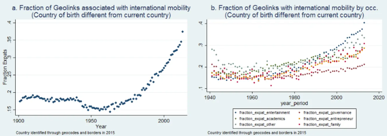
8. In all occupations, there has been a rise in international mobility since 1960. The fraction of locations in a country different from the place of birth went from 15% in 1955 to 35% after 2000.
9. There is no positive association between the size of cities and the visibility of people measured at the end of their life. If anything, the correlation is negative.
10. Last and not least, we find a positive correlation between the contemporaneous number of entrepreneurs and the urban growth of the city in which they are located the following decades; more strikingly, the same is also true with the contemporaneous number or share of artists, positively affecting next decades city growth; instead, we find a zero or negative correlation between the contemporaneous share of “militaries, politicians and religious people” and urban growth in the following decades.
There is currently a growing number of datasets allowing for the documentation of historical facts. A recent approach has focused particularly on historical individuals, who we call in this text notable people. This approach was pioneered by Schich et al. (2014). The authors automatically collected the years and locations of birth and death for 150,000 notable people in history using Freebase, a Google-owned knowledge database. de la Croix and Licandro (2015) built a sample of 300,000 famous people born between Hammurabi’s epoch and 1879, Einstein’s birth year from Index Bio-bibliographicus Notorum Hominum, to estimate the timing of improvements in longevity and its role in economic growth. Recently, Yu et al., (2016) also used Freebase and assembled a manually verified dataset of 11,341 biographies existing in more than 25 languages in Wikipedia. Our paper extends these approaches. We compile the largest possible database of notable people rather than focusing only on “very famous” individuals, because we are ultimately interested in detecting the statistically significant local economic impact of these individuals. It actually turns out that weighting individuals with measures of their impact does not make a big difference, which ex post justifies our collection of information on hundreds of thousands of lesser known artists, business people and local rulers, famous enough to have been listed and described somewhere on the internet or in various rankings, but yet left out of the vast majority of internet sources.
To this end, we use two different, yet complementary approaches to obtain names of and information on notable people. One is also based on Freebase, and allows us to collect information at a large scale for 938,000 individual profiles over 4,000 years of human history, after a careful examination of homonyms and the elimination of duplicates. We refer to this method as “top-down”, since the information on names is centralized in Freebase. The second method is based on a systematic search from various categories in Wikipedia pages to identify notable people and is refered to as a “bottom-up” approach. This
results in a list of about 1 million individuals that considerably overlaps with the “top-down” approach, and eventually adds another 280,000 names to the Freebase results.
These individuals are then matched with their respective Wikipedia biographies in English, from which we extract a large amount of biographical information through a careful and manually verified se-mantic analysis. We categorize people according to gender, nationality, and their three main activ-ities/occupations according to an ad hoc classification system consistent throughout history. Other key information such as birth year, death year, birth place, place of death and most importantly all geographical linkages (GeoLinks thereafter) mentioned in the biography in between birth and death, have been systematically collected where available. A total of 3.5 million geographical linkages have been gathered and analyzed.
We also attempt to measure these individuals’ impact on various economic outcomes. The visibility of each individual’s page is probably a better proxy of his or her impact than the number of pages viewed over the past years (the alternative approach pionneered by Yu et al., 2016). Therefore, we use a simple impact measure compiled using a combination of the number of words in the Wikipedia page and the number of languages into which the page has been translated. The implied ranking is disclosed in the text and its Appendix, both in an overall ranking and in rankings by categories. Alternatives are explored and correlations between them analyzed.
We then match notable people with cities using a unique global historical population database com-posed of new Census data from 17 countries on 5 continents, the Urbanisation Hub-Bairoch-Bosker city population data between 800AD - 1800AD, the Lincoln population data 1794 - 2005 for 24 other cities in the world, and the United Nations (UN) population database since 1950. For each country and within each period, we select the 30 largest cities at a time for countries with a landsize of less than approximately 300,000 square kilometers and for the 50 largest cities for larger countries with a landsize larger than 300,000 square kilometers. The landsize threshold is more time invariant than any other population criterion and the number of cities retained permits that 50% of 3.5 million locations assembled in the database over the period 800AD-2015AD lie within 50km of the nearest city. In the last period of the sample (1950AD-2015AD), the UN population database even allows us to have 50% of the locations within 13km of the nearest city.
In this paper, we carefully document the data search and procedures to extract the relevant informa-tion. We then explore the datasets, provide a number of descriptive stylized facts and finally provide descriptive, non-causal associations of the role of notable people on city growth.
1 Data collection
1.1 A list of individuals from Freebase then matched with Wikipedia pages
(“top-down” approach)
We exploit information on Freebase as documented in Schich et al. (2014). Freebase is a Google-owned knowledge database providing a list of notable individuals known to have existed. This list comes from a variety of web sources, including Wikipedia, the Internet Movie Database, Allocine, and others. The link we refer to is: https://www.freebase.com/people/person?instances=. The procedure includes several steps.
his/her birth date (if available). As of January 2015, when we accessed the list, Freebase contained precisely 3,440,707 notable people. However, many names were duplicates, or mistakenly added. A subset of nearly 407,000 irrelevant observations, corresponding either to pure html codes, movie titles, ships such as HMS Titanic, names in non-Latin alphabets (overall, this eliminates around 3,000 names that appear in Chinese/Korean characters, in Greek or Cyrillic alphabets) or even numbers instead of full regular names have been identified and then automatically dropped out of the initial dataset. This step leads to a sample of 3,033,469 notable people.
2. We then match these 3 million names with their corresponding Wikipedia pages in English. The matching process was more easily facilitated when using the birth date, where available, especially for homonyms. Overall, 46% (1,391,718 observations) include a birth year. The matching process achieved a lower success rate for people with no such birth information, i.e. when the matching process was based on the full name only (see next point). Missing birth dates represent 54% of the sample (1,641,751 observations).
3. There are several homonyms in the database. When Wikipedia detects homonyms it either provides a list of names with birth dates1 or directly takes the user to the page of the most famous homonym e.g. for Ray Charles (https://en.wikipedia.org/wiki/Ray_Charles), via the following sentence and link : “For other uses, see Ray Charles (disambiguation). In this second case the link refers to a list of homonyms with a link to each one’s respective page. In both cases, in order to capture as many homonyms as possible from Freebase we match both the full name and the birth year. For homonyms with no birth information in Freebase, we only consider the page corresponding to the most famous homonym instead of collecting all pages mentioned in the list described before (first case).
Among the individuals with birth year information, approximately 30% do not have a Wikipedia page in English, 868,266 have a unique link to a page in English, while 154,349 are not matched. Among these pages, 76,000 must be disambiguated as they contain more than one link. This leads to a first group of names. Among individuals with no birth year information, 313,308 come up with a unique link to a Wikipedia page in English, but only 106,646 refer to an individual (and not to a list of homonyms, concepts, etc.). Of these, 37,854 are not duplicates with respect to the first group detailed above (with birth year information) and are therefore included in the final sample.
At the end of the process, 964,245 individuals are matched with their Wikipedia biography, which we downloaded as of December 2015.
1.2 A list of individuals using Wikipedia categories (“bottom-up” approach)
To be exhaustive and consistent, we also use Wikipedia directly, which classifies most individual pages by birth date. A secondary independent dataquest is run automatically from birth dates between 1500BCE to 2015AD; a complete list of categories is assembled; virtually all of these categories include additional lists of people. Each of these is scanned to obtain more names with a page in English. We obtain a total of 1,176,812 names including 897,310 names in common with names identified using the “top-down” approach and 279,531 distinctly new names.
We then merge the two databases (“top down” and “bottom up”) using the url of each individual (https://en.wikipedia.org/wiki/[first name+last name]. Figure 1 describes the process and the final outcome. The final database includes 1,243,776 notable people.
FREEBASE : 3,033,469
With Birth year : 1,391,718 With no Birth year : 1,641,751
Matches : 868,266 No Match : 154,349 Matches : 106,646
Matches from Disambiguation : 18,792
Total matches : 993,704
Net matches 897,310 Pages from Wikipedia birth categories
Our Database : 1,243,776 = 964,245 (Freebase) + 279,531 (Wikipedia)
Figure 1: Organization chart
1.3 Individual characteristics
In this subsection we analyze the source code of each Wikipedia page to extract basic information about dates and locations for birth and death, occupations, citizenship and gender. These individual characteristics are either identified from the Infobox (fixed-format table at the top right-hand corner of biographies), from the Abstract, or from the Categories section. 398,830 (36.05%) individuals have no Abstract and therefore we extract information from the Main text.
Figure 2 shows the different parts of the Wikipedia page of Ray Charles. See his full page in the Appendix.
Birth and Death Dates Information on an individual’s date of birth and death is typically available in three different sections of the Wikipedia biography: i) Infobox, ii) Abstract/Main text and iii) Categories section, which is located at the bottom of the page.
We therefore get a maximum of three birth dates per individual of which 1,063,637 come from the Categories section, 669,405 were found in the Infobox and 951,147 were extracted from the Abstract/Main text. Some are misreported but the alternative birth dates allow for a correction: among observations without missing dates, the concordance rate between birth dates coming from the same biography is at around 97.3%. Similarly, we found 498,065 dates of death in the Categories section, 232,584 in the Infobox and 383,088 in the Abstract/Main text. The concordance rate between dates of death coming from the same biography is at around 98.4%.
We end up with 1,073,585 birth years and 499,980 death years. Missing death years correspond either to an unreported death year or to an individual still living in 2015 (a large fraction of our database : 59%). Note also that we have 144,804 individuals with no birth information available regardless of the three sources used. Among those individuals, 21,581 have information available on their death. Places of Birth and Death Places of birth and death may both be found in the Infobox and/or in the main body of the text (Main text). We first analyze the information coming from the Infobox and then consider the Main text as an alternative source of information when either the Infobox is missing or the relevant information has not been detected in the Infobox. In this case, we use keywords such as “born in/at” or “died in/at” to find place of birth and death. Most locations of an individual’s birth and death are associated to a latitude and a longitude (hereafter we use the word geocoded), which we then extract.
Citizenship/Gender Information about citizenship is usually present in the Infobox and in the Abstract/Main text. We use both sources in order to minimize the number of missing values. On rare occasions, when there is more than one citizenship/country mentioned in the Abstract, we consider the citizenship appearing first as that individual’s citizenship. After thorough manual verification, it appears that this information always appears first in the Abstract section (as illustrated below in Ray Charles’ biography).
For gender we also use the Abstract/Main text and check for the presence of pronouns (he/she) and possessive adjectives (his/her) in the text. We consider a person to be female (male) if “she”/ “her” (“he”/ “his”) is found in the summary. In case we detect both masculine and feminine pronouns or possessive adjectives, we select the first pronoun that appears as the one identifying the person’s gender. This method did not prove efficient for short biographies which do not contain any pronouns or possessive adjectives. Overall, women account for only 15.7% of the sample, while men represent the largest share (78.5%) and we failed to identify the gender information for only 5.8% of all biographies analyzed. However, a careful visual inspection of this latter category indicates that missing genders are predominantly males.
Occupations We determine occupations by locating linking verbs such as “was a”/“is a”/“was the”/“is the” in the Main text: for instance, “Ray Charles was an American singer, songwriter, musician, and composer”. Occupations are then grouped into 6 categories: Academics (studies, education), Entertain-ment (arts, literature/media, sports), Entrepreneur (business, inventor, worker), Family, Governance
Occupation A1 Frequency Share Academics (studies, education) 110,610 9.0 Entertainment (arts, literature/media, sports) 736,626 60.0 Entrepreneur (business, inventor, worker) 59,028 4.8
Family 11,813 1.0
Governance (law, military, religious, politics, nobility) 285,514 23.3
Other 23,712 1.9
Total 1,227,303 100.0
Table 1: Occupations (level of aggregation A - six categories)
Occupation B1 Frequency Share Arts 241,042 19.6 Business 48,974 4.0 Education 36,542 3.0 Family 11,813 1.0 Inventor 4,783 0.4 Law 28,585 2.3 Literature/media 103,421 8.4 Military 40,516 3.3 Nobility 20,013 1.6 Other 23,712 1.9 Politics 160,696 13.1 Religious 35,104 2.9 Sports 392,163 32.0 Studies 74,068 6.0 Worker 5,271 0.4 Total 1,226,703 100.0
Table 2: Occupations (level of aggregation B - 15 categories)
(law, military, religious, politics, nobility) and Other. Tables1and2 provide a few summary statistics of the entire database. See the full list of occupations collected and sorted in the Appendix.
Table 3 summarizes the information that has been collected so far and informs us about the location where the information was found in the Wikipedia biography.
Visibility Factors Various “influence weights” are built, based on specific page characteristics com-bining the length of the page (in words), the number of translations of the page and some additional information such as the number of footnotes, categories, headlines, links, etc. Futher details about these are provided in Section 2 below. As argued in the introduction, many other sources, depending on the type of study envisaged can serve as a proxy for the visibility factor. Our measures fit well our purpose, which is to detect the local economic impact of the individuals present in the database.
The number of pages viewed in recent years is a potential indicator that has been favored by Yu et al. (2016), and would be very useful if we were interested in studying contemporary individuals (living artists, athletes). The number of internet pages (backlinks) linking to a Wikipedia biography could also be an indicator. The latter information would be interesting per se as a measure of the relevance of these biographies. For our purpose, the information on the length and complexity of a Wikipedia
Individual variables Location within the Wikipedia biography Available Birth & Death Dates Abstract/Main text + Categories + Infobox 1,073,585 & 499,980 Birth & Death Places Main text + Infobox 842,926 (67.77%) & 235,514 (46.25%)
Occupation Abstract/Main text 1,183,971 (95.19%) Gender Abstract/Main text 1,149,899 (92.45%) Citizenship Abstract/Main text + Infobox 1,090,190 (87.65%)
Shares for death dates and death places are computed using the number of dead people only, i.e. 509,181 observations.
Table 3: Number of individuals with available information
biography and the number of links leading outwards to the Internet is still the most appropriate: we presume that individuals who have a Wikipedia biography and another biography elsewhere on the internet have had precisely the impact we attempt to detect. Of course, we may want to compare an individual’s visibility relative to others in their respective birth cohort where relevant.
1.4 Geographical Wikipedia linkages (GeoLinks)
An important improvement of the present work compared to other articles quoted above is our in-depth and careful analysis of GeoLinks present in individual Wikipedia biographies. This analysis provides detailed and reliable information about these different places where famous people live (lived) and/or interact with (interacted with) over the course of their lifetime2.
To collect such information we copy all hyperlinks found in each page and make a distinction between links found in the abstract and links coming from the Main text. Hyperlinks, by definition, lead to other Wikipedia Pages (Wikilinks), which we extract and parse. Wikilinks with geographical coordinates (longitude/latitude), are potential GeoLinks such asAlbany, Georgia where Ray Charles was born.
We discard countries, regions or provinces that are locations with geographical coordinates as our goal is to match notable people with places at the city level (see below). There are also pages containing coordinates that do not correspond to locations, but to individuals. These pages provide the coordinates of their resting/burial place. For instance, the wikilinkRonald Reaganappears in Charles’ Wikipedia page. Charles performed for Reagan’s second inauguration in 1985. Ronald Reagan is considered by our code as a location because his page provides the coordinates of his resting place (Ronald Reagan Presidential Library, Simi Valley, California, 34.25899°N 118.82043°W). We can identify these wikilinks that contain coordinates but which are not locations and therefore exclude them.
A GeoLink may not necessarily point to places where famous people at some point moved to, lived in or even just visited. After careful verification of hundreds of cases3, it appears that a significant fraction of these GeoLinks refer to parents/family, or to a place where they lived, originated from, etc. This information might be relevant for some uses, but is not relevant in analyses of an individual’s direct impact, so we keep both but separate them out, distinguishing between two types of GeoLinks: those having a connection with family and those with no obvious link to family, using keywords such as
2We will use thereafter either the present or preterit tense to talk about present and past linkages respectively. 3These verifications are available from authors upon request.
Wikilinks GeoLinks Countries/Regions Resting Place Family Post-mortem 7,184,575 4,878,455 1,829,400 32,915 398,3331 363,318
(67.90%) (25.96%) (0.47%) (5.65%) (5.06%)
Table 4: Number of identified GeoLinks
“sister”, “father”, “brother”, etc. contained in the same sentence to allocate them into the first category. Other GeoLinks refer to post-mortem events and can safely be dropped out of the sample. These are quite frequent for artists (e.g. links to museums where exhibitions of their work take place post-mortem ) or scientists (e.g. honorary awards, buildings named in his/her honor). We consider a location to be post-mortem whenever a GeoLink is pointed out after an individual’s date of death and is present in a sentence where keywords such as “died/buried/...” are present.
Table 4 shows that among all 7,184,455, Wikilinks extracted 26% correspond to either countries or regions, 0.5% refers to a person instead of a location, 5.7% are places visited by family members and 5.1% are post-mortem locations. These cases are not mutually exclusive. In all, we detected 4,878,455 proper and usable GeoLinks.
Places are either located in the Abstract or in the Main text. Therefore, in order to keep a chrono-logical path of places visited, we keep either the Abstract or the Main text depending on the number of places contained in both sections. We extract places from the section containing the largest number of GeoLinks. The Abstract is chosen arbitrarily in the case of a tie. On average, individuals have 5.7 GeoLinks in the Main text and only 2.4 in the Abstract.
We detail here the places visited by Ray Charles (1930-2004) as it was identified by our automatic detection procedure. Charles was born in Georgia and grew up in Florida before reaching cities like Seattle, Philadelphia, New York and Los Angeles. Along with Table5providing the GeoLinks, Figure5
in Appendix shows the screenshots of the different sections of his Wikipedia page including GeoLinks. Figure 3 shows the map of places visited by Ray Charles according to his Wikipedia page. It is important to report that not all GeoLinks refer to city names. Some point to cultural events, museums, opera houses, theaters, universities, schools, stadiums or sports events such as Olympic games, etc.. Those links have coordinates and are added to GeoLinks. In this example, Ray Charles had two contacts with the city of St. Augustine, Florida, through a school first (Florida School for the Deaf and the Blind) and a radio station (WFOY) based in the same city. This is important information to consider as sampled individuals have had contact with these cities through these institutions.
Order of appearance GeoLinks in the biography
1 Albany, Georgia 2 Greenville, Florida 3 St. Augustine, Florida
4 WFOY (radio station), St. Augustine, Florida 5 Jacksonville, Florida
6 Ritz Theatre (Jacksonville) 7 LaVilla, Jacksonville, Florida 8 Orlando, Florida
9 Tampa
10 Seattle, Washington 11 Overtown (Miami) 12 St. Petersburg, Florida 13 The Apollo Theater 14 Uptown Theater (Philadelphia) 15 The Newport Jazz Festival 16 Beverly Hills, California
Table 5: GeoLinks of Ray Charles
We show here, as another example, the trajectories of a person known for having been very mobile over the course of his life: Desiderius Erasmus (1466-1536AD) in Figure4. Erasmus was born near Rotterdam (Netherlands: 1) with some controversy about whether he originated from Gouda (Netherlands: 2). Erasmus has an indirect (weaker) link with at least two different GeoLinks. First, with the city of Zevenberger (Netherlands: 3) which is the place of birth of his grandfather and second with the city of Deventer (Netherlands: 4) where his oldest brother went to a famous school. Both places are family-related GeoLinks and are therefore in blue on the map. As previously explained, these two locations have been dropped from the list of GeoLinks. According to Wikipedia, the connection between Erasmus and Nuremberg (Germany: 5) is through a Portrait of him by Albrecht Dürer in 1526 which he engraved in that city. Next, Erasmus was tutoring in Paris (France: 6). Paris was mentioned no less than eight times in Erasmus’ biography. Then he moved from Paris to Cambrai (France: 7) when he became a secretary to the Bishop of the city. Then he returned to Paris to study there at the University (France: 8). After Paris he moved to Leuven (Belgium: 9) where he became a lecturer at the Catholic University. His next move was from Leuven to Cambridge (United Kingdom: 10) where he held the position of Professor of Divinity at the University from 1510 to 1515. In 1506, he graduated as Doctor of Divinity from the Turin University (Italy: 11) and also worked part time as a proofreader at a publishing house in Venice (Italy: 12). Erasmus then emigrated from Venice to Basel (Switzerland: 13), a city that he left in 1529 to settle in Freiburg im Breisgau (Germany: 14) where he eventually died at the age of 69. Finally, we report on Figure5the birth to death trajectories on a smaller sample (1/20th of individuals with initials A and some B) and the barycenter of individuals in the database by time period and their dispersion, from individuals born before 500AD (yellow ellipses) to the most recent period (darker ellipses). Ellipses are constructed from the standard deviations of longitude and latitude. One can observe first, on top, the concentration of locations around an axis Europe-North America and second, in the bottom part of the Figure, the slow movement of the sample from the Middle-East to Western Europe with a barycenter in France during the XVIth and XVIIth centuries and towards North America, returning to the South-East in the last two centuries with the emergence of Africa and Asia (see Section 2). Coïncidentally, in 1637 (year of “Discours de la Raison by René Descartes), the exact barycenter of the base was actually in the small village of Colombey-les-Deux-Eglises (Champagne), where Charles de Gaulle bought his family house and died. Since the 1970s, the barycenter oscillates between Morocco, Algeria and Tunisia.
Figure 5: Top: birth to deaths trajectories of 1/20th of individuals. Bottom: barycenter of individuals in the database by time period and their dispersion from individuals born before 500AD to individuals born after 1900AD.
1.5 Matching procedure of GeoLinks to Time Periods
For subsequent descriptive analyses, we often group individuals into aggregate time categories. At the highest agregation level we use 5 large historical periods (<500AD; 501-1500AD; 1501-1700AD; 1701-1900AD; 1901-2015AD); see for instance the different maps of Europe and the world in Appendix A. We also use, in the econometric analysis of later sections, 66 Time Periods of varying length constructed as follows: individuals born before 1AD are divided into three groups, due to sample size (born before 500BCE, born between 501BCE and 250BCE, born between 249BCE and 0); periods of 50 years between 1AD and 1700AD; periods of 25 years between 1701AD and 1800AD and periods of ten years between 1801AD and 2015AD. These varying lengths of time capture the “accelerating history” phenomenon and reduce the disparities in the number of individuals across time periods.
The most important methodological choice here is to attribute to each GeoLink one or two of these Time Periods, as follows. Information on birth and death allows us to calculate the lifespan of each individual. We also estimate the mean lifespan according to each birth year or each Time Period, for both male and female individuals. When either the birth or death information is missing, we therefore impute lifespan based on the relevant Time Period of the gender category of the individual. Once done, we count the number of GeoLinks for that individual and use it to calculate the steps of a grid of the entire lifespan, as a proxy for the time elapsed between two successive GeoLinks. For people still alive in 2015, we use their current age in 2015 rather than their lifespan. Then, if a GeoLink is estimated to start in year a and end in year b, we assign that GeoLink to Time Period n if any year in the interval (a, b) intersects that Time Period .
The first GeoLink of a given individual should in principle be his or her birthplace and the last GeoLink should be his or her place of death. This might not always be the case, however, and in hundreds of manually verified cases, the GeoLinks were sometimes indicating high-schools or other places. For these people, we therefore add a first GeoLink with the birthplace when available in the Infobox, or a last GeoLink with the place of death when available from the same source.
1.6 Validity of the extraction procedure
The extraction procedure presented above has been checked by a series of manual verifications based on 4 randomly selected sub-samples of extracted biographies (853 in total). Both the individual character-istics (birth and death dates, places of birth and death, citizenship, gender, occupation) and GeoLinks automatically extracted by our code have been cross verified. At each round of verification, the code was modified and re-run on the entire sample. We present in Table 6 detailed statistics about the different iterations. The rate of errors on variables is generally decreasing (and ends up being lower than 7%) and the one on GeoLinks is limited (lower than 10%). Further improvements of the code are envisaged to improve this systematic detection procedure.
Data scientists and statisticians have introduced the concept of random dataset in which any information is subject to error and is potentially weighted by a probability of error. This will be our next step in future versions of the work. In the remaining sections we present some stylized facts as well as some correlations obtained between the various statistics generated by our Wikipedia extraction procedure and city population data as another ex post check of the quality of the database.
GeoLinks Individuals % Residual errors on % Residual individual characteristics errors on places Round 1 452 114 24.5 20.1 Round 2 711 113 35.3 14.3 Round 3 849 152 13.8 11.4 Round 4 1316 81 6.17 9.12
Table 6: Manual verifications: performance statistics in each round
2 Facts on notable people
2.1 Size of cohorts in the sample
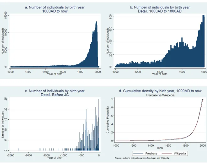
The sample is unbalanced across birth years, with an exponential growth of the sample size over time. The first individual in the database was born in 2285BCE, but the median individual was born in 1943 AD (column I). Only 1% (1099 individuals) were born before 1330. The composition of individuals not selected from Freebase (“top-down” approach) but from Wikipedia (“bottom-up” approach) is not very different in terms of years of birth. The size of a cohort for a given year in the database varies from 0 or 1 to as much as 157,735 in the most recent years.
Variable Obs Mean Std. Dev. Database Min Max P1 P10 P25 P50 P75 P90 P99 1,073,568 1908 140.305 Full sample -2285 2015 1381 1820 1894 1943 1971 1985 1994 Birth year 139,965 1902 164.046 Wikipedia -1570 2015 1220 1811 1893 1944 1974 1990 1997 933,603 1909 136.369 Freebase -2285 2015 1406 1821 1894 1943 1971 1985 1993 499,959 1886 235.683 Full sample -2566 2015 689 1712 1889 1954 1993 2008 2015 Death year 80,997 1771 382.134 Wikipedia -1991 2015 254 1278 1730 1932 1985 2007 2015 418,962 1908 187.17 Freebase -2566 2015 1075 1790 1899 1958 1994 2008 2014
Table 7: Statistics on birth year and death year
Figure 6: Cohort size in the database of individuals, Freebase/Wikipedia samples merged (first three charts) or kept separated bottom left chart
2.2 Average longevity
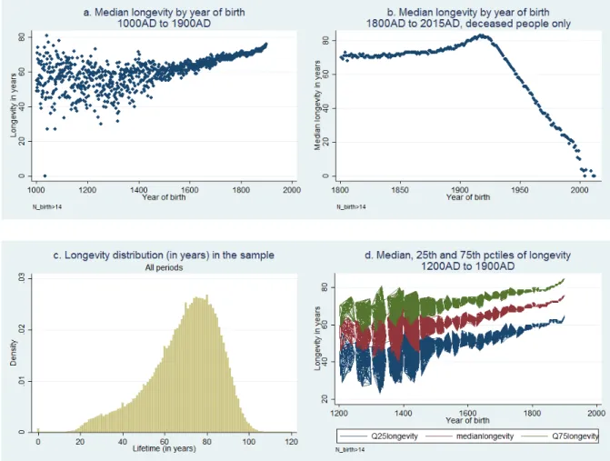
Longevity is expressed in years and computed as the difference between year deceased and year of birth, each of these itself estimated (see Section 1) from all available information on birth and death coming from Wikipedia categories, the Infobox and the Abstract/Main text. We first present the overall distribution for all years, then for the most recent period. For individuals born after 1900 and for
whom a death has been recorded, lifespan is necessarily declining over time. For individuals born in 2000, average lifespan must be necessarily computed using 2015 as a reference year along with his/her birth year. As found in de la Croix and Licandro (2015), we observe that the steady improvements in longevity start with cohorts born around 1600.
Note: After 1900, a majority of individuals is still alive and the series is unreported, since by construction life duration decreases to zero as years of birth are closer to 2015.
Figure 7: Longevity in years
Interestingly we see from Figure7a and7d that the lifespan variance across individuals also decreased over the sample period; although it rose again after 1830, presumably because of an increase in people of an older age.
2.3 Average visibility: all individuals
The large number of individuals in the database is a distinctive feature of our work, as compared to previous attempts. This large number necessarily implies that most individuals have little visibility on the web. Yet, they may contribute to the social, economic or cultural development of their area of residence.
We start by providing an overview of the distribution of the number of words and translations of the biography. All distributions, Freebase and Wikipedia, are very skewed. Pages that were collected using Freebase are on average longer and more translated than these extracted directly from Wikipedia following the “bottom-up” approach. Indeed, the additional pages from the Wikipedia search bring many individuals with little visibility. Another interesting finding is the time evolution of these two variables: as time goes on, they tend to decrease suggesting that history has kept memory of the most notable figures, while more recent individuals are more numerous and on average less impactful.
Figure 8: Components of visibility: distributions of number of translations of pages and number of words, time evolution and correlations
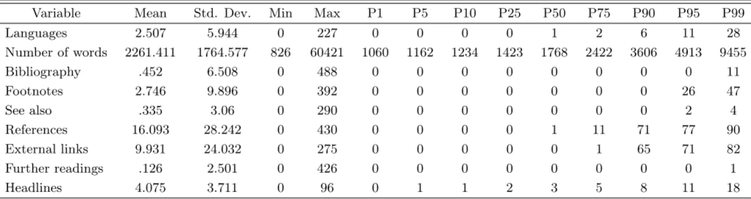
Both indicators (number of words and number of page translations) are correlated with many other variables, such as “number of bibliography items, number of footnotes, number of “See also”, number of references, number of external links, number of “Further readings”, or number of “Headlines” as indicated in Table8.
Variable Mean Std. Dev. Min Max P1 P5 P10 P25 P50 P75 P90 P95 P99 Languages 2.507 5.944 0 227 0 0 0 0 1 2 6 11 28 Number of words 2261.411 1764.577 826 60421 1060 1162 1234 1423 1768 2422 3606 4913 9455 Bibliography .452 6.508 0 488 0 0 0 0 0 0 0 0 11 Footnotes 2.746 9.896 0 392 0 0 0 0 0 0 0 26 47 See also .335 3.06 0 290 0 0 0 0 0 0 0 2 4 References 16.093 28.242 0 430 0 0 0 0 1 11 71 77 90 External links 9.931 24.032 0 275 0 0 0 0 0 1 65 71 82 Further readings .126 2.501 0 426 0 0 0 0 0 0 0 0 1 Headlines 4.075 3.711 0 96 0 1 1 2 3 5 8 11 18
Table 8: Number of words per page, translations and other visibility indicators
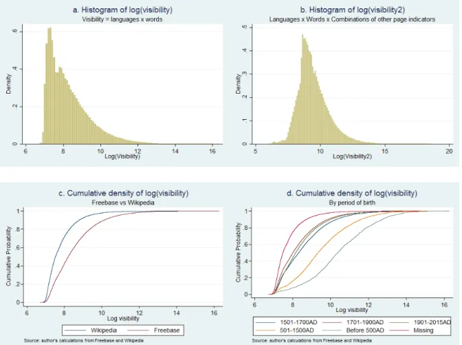
out that the most basic combination leads to relatively sensible rankings. Indeed, the log of the product of the number of translations (+1) times the number of words in the Wikipedia biography leads to an indicator, called visibility, which is represented in Figure 9a. An alternative ranking is composed as the first index (visibility) multiplied by the log of the sum of all of the other variables described in the previous paragraph. The correlation between both indicators is 0.90 in levels and 0.88 in logs. The second distribution (Figure 9b) is more symmetrical than the one based on the basic visibility index positively skewed. The distribution in Figure9is based on visibility and will be used in the rest of the paper as it best reflects the skewness of visibilty in the database (already captured by the fact that we use logs; in levels, the distribution is extremely skewed leftward). It is also no surprise that visibility is higher when individuals are selected from Freebase given that they have shorter pages and fewer translations, as indicated above (Figure9c); and when they belong to older cohorts (Figure9d).
Figure 9: Visibility indices
2.4 Visibility: women
Over time, an interesting pattern emerges, a U-shape curve, with a local minimum at around 1700 (Figure 10a). This might be attributable to a composition effect (e.g. fewer and fewer individuals in the Family group and more and more in the Artists and Sports categories). However, unreported graphs, available from authors upon request, reveal that the U-shape pattern emerges for all six groups of occupations. At the end of the observation period, the female share is at around 0.25. We see also that females are less visible than males; there is a clear first order stochastic dominance in Figure10b as expressed by the c.d.f. of visibility.
Occupation Obs Mean Std. Dev. Min Max P1 P10 P25 P50 P75 P90 P99 Entertainment 698,704 1937.053 85.996 -1557 2015 1610 1877 1921 1958 1979 1988 1995 Academics 130,075 1886.951 145.864 -1570 2015 1428 1803 1870 1921 1947 1963 1989 Entrepreneur 76,262 1879.818 108.782 -550 2015 1510 1777 1841 1907 1949 1966 1987 Family 21,338 1767.293 323.474 -1398 2015 191 1422 1737 1886 1945 1972 2000 Governance 303,263 1848.069 205.971 -2285 2015 862 1709 1833 1905 1946 1962 1986 Other 39,721 1893.812 151.736 -915 2015 1298 1814 1882 1922 1959 1979 1993
Table 9: Summary statistics: birth year by occupations
Figure 10: Share of women in different occupations throughout history
2.5 Evolution of occupations
We now investigate the share and visibility of our different occupations. As indicated, we have three levels of aggregation for occupations. Table9shows the distribution of the highest level of aggregation (six categories).
Figure 11a shows the evolution of these categories over time, for people born before 1990 (e.g. being at least 25 y.o.). The series sum up to slightly more than 1 since an individual may be in more than one category (e.g. Academics and Entrepreneur; the only exclusion is that an individual cannot be in Governance and another category). As visible, the post-1950 period sees the rise of the “Entertain-ment category”, which by far dominates the database. The Governance category, most present until the beginning of the XIXth century, decreases after the 1840’s cohort and drops further after 1950 (mechanically since these are shares, but gross numbers also decrease).
The middle part of the graph shows the evolution of categories for the intermediate level of aggregation (15 categories). In particular, it shows that Sports rose in two periods: for the birth cohorts between 1850 and 1870, with the emergence of sports contests in the second half of the XIXth century culminating with the first modern Olympic Games in 1896 and the first Tour de France in 1904. Interestingly, as Figure11c shows, there has been a race between Sports and Art and Literature/Media between birth cohorts 1860 to 1950 with the final victory of Sports after 1950. The Figure11b shows the cumulative
density of the visibility index retained; most activities are similar in terms of prominence except Family, which tends to be over-represented at large visibility levels.
2.6 Detailed lists of individuals in the database: top people and examples
in various places
We now present the list of individuals in various categories. The top of each table lists the top 20 individuals in the category, and then sample individuals in the top decile, top quartile, median, third quartile and last decile, to give an overview of the composition of the database. All other categories are reported in Appendix.
Cat. rank Ov. rank Name Birth Death Citizenship Occupation B1 Occupation B2
Top 20 individuals
1 3 Jesus 0 30 . Family religious
2 5 Napoleon Bonaparte 1769 1821 France military politics 3 6 Winston Churchill 1874 1965 England politics politics 4 9 Adolf Hitler 1889 1945 Austria politics politics 5 10 Joseph Stalin 1878 1953 Russia politics politics 6 12 Mahatma Gandhi 1869 1948 India politics politics
7 13 Mahomet 570 632 . religious Other
8 14 William Shakespeare 1564 1616 England lit lit 9 18 Alexander The Great -356 -323 Greece nobility nobility 10 19 Mustafa Kemal Atatürk 1881 1938 Turkey military military 11 20 Franklin D. Roosevelt 1882 1945 US politics politics 12 21 Abraham Lincoln 1809 1865 US politics politics 13 23 George Washington 1732 1799 US politics military 14 26 Charlie Chaplin 1889 1977 England arts arts 15 27 Vladimir Lenin 1870 1924 Russia politics politics 16 28 Charles de Gaulle 1890 1970 France lit politics 17 30 Albert Einstein 1879 1955 Germany studies studies 18 32 Karl Marx 1818 1883 Germany studies studies 19 41 Theodore Roosevelt 1858 1919 US politics lit 20 43 Vincent Van Gogh 1853 1890 Netherlands arts arts
Top decile (random sample)
25019 101995 Karl Freiherr Von Müffling 1775 1851 Germany military
25021 102007 Custodio García Rovira 1780 1816 Spain politics arts 25020 102008 Jacques de Billy 1602 1679 France religious studies 25023 102023 Antoine-Vincent Arnault 1766 1834 France arts arts 25022 102026 Ebbo 775 851 Germany religious religious
First quartile (random sample)
62554 268965 Charles L. Hutchinson 1854 1924 US business business 62553 268967 Emil Johann Lambert Heinricher 1856 1934 Austria studies studies 62550 268969 George Douglas, 16th Earl of Morton 1761 1827 US Family nobility 62552 268977 Paul Morgan (actor) 1886 1938 Austria arts arts 62551 268983 Emil Barth 1879 1941 Germany politics worker
Median (random sample)
125104 591207 Edmund Frederick Erk 1872 1953 US politics politics 125102 591276 Ripley Hitchcock 1857 1918 US lit arts 125106 591293 Alexis Lesieur Desaulniers 1837 1918 Canada law politics 125105 591336 Anna Maria Hilfeling 1713 1783 Sweden arts arts 125103 591347 Edward Garrard Marsh 1783 1862 England lit religious
Third quartile (random sample)
187655 931626 William Cole (scholar) 1753 1806 England education education 187656 931829 A. W. Andrews 1868 1959 England studies lit 187658 931846 Thomas Nash (Newfoundland) 1765 1810 Ireland worker Other 187657 931911 Hugh Aiken Bayne 1870 1954 US Family law 187654 931912 Samuel Backhouse 1554 1626 England business politics
Last decile (random sample)
225187 1121555 Edward Hopkins (politician) 1675 1736 Ireland politics education 225185 1121647 Braxton Lloyd 1886 1947 US studies politics 225188 1121709 Stephen Furniss 1875 1952 Canada politics politics 225189 1121712 Ida Holterhoff Holloway 1865 1950 US arts arts 225186 1121786 Robert Henry Blosset 1776 1823 England law military
Cat. rank Ov. rank Name Birth Death Citizenship Occupation B1 Occupation B2
Top 20 individuals
1 1 Barack Obama 1961 US politics education 2 2 Ronald Reagan 1911 2004 US politics arts 3 4 George W. Bush 1946 US politics business 4 7 Nelson Mandela 1918 2013 South Africa politics politics 5 8 Michael Jackson 1958 2009 US arts arts 6 11 John F. Kennedy 1917 1963 US politics politics 7 15 Pope Francis 1936 Argentina religious religious 8 16 Cristiano Ronaldo 1985 Portugal sports sports 9 17 Pope John Paul Ii 1920 2005 Poland politics religious 10 22 Roger Federer 1981 Switzerland sports sports 11 24 Lionel Messi 1987 Argentina sports sports 12 25 Novak Djokovic 1987 Serbia sports sports 13 29 Hillary Rodham Clinton 1947 US politics politics 14 31 Bill Clinton 1946 US politics politics 15 33 Pope Benedict Xvi 1927 Germany politics religious 16 34 Che Guevara 1928 1967 Argentina politics politics 17 35 Elvis Presley 1935 1977 US arts arts 18 36 Mao Zedong 1893 1976 China politics politics 19 37 Hugo Chávez 1954 2013 Venezuela politics politics 20 38 Rafael Nadal 1986 Spain sports sports
Examples at the top decile
81954 113355 Evan Jenkins (politician) 1960 US politics politics 81956 113358 Anton Golotsutskov 1985 Russia sports sports 81957 113361 Alphonse Leweck 1981 Luxembourg sports sports 81953 113365 Lazar Ristovski 1952 Serbia arts arts
Examples at the first quartile
204889 283176 José Greci 1941 Italy lit arts 204888 283204 Valeria Solarino 1979 Italy arts arts 204887 283206 Mark Preston 1968 Australia business business 204886 283212 Lev Dobriansky 1918 2008 . education education
Examples at the Median
409775 567684 Jeanette Lunde 1972 Norway sports sports 409774 567752 Cristian Andrés Campozano 1985 Argentina sports sports 409776 567799 Clifford Peeples 1970 Ireland religious politics 409773 567823 Stephen Adams (business) 1937 US business business
Examples at the third quartile
614663 875000 Dorice Reid (baseball) 1929 US sports sports 614660 875029 Birger Wernerfelt 1951 Denmark studies business 614661 875091 Les Phillips 1963 England sports sports 614662 875145 Casey Henwood 1980 New Zealand sports sports
Examples at the last decile
737592 1080475 Philip Gardiner 1946 Australia politics politics 737595 1080596 James A. Andersen 1924 US politics law 737596 1080687 Jeanette Kuvin Oren 1961 US arts arts 737594 1080777 Bruce Martyn 1930 US sports lit 737593 1080969 Claude Legris 1956 Canada sports sports
2.7 Geographical density through history
Finally, the sample is predominantly drawn from the Western World (Europe and North America) with, however, a rise of other continents, mostly Asia and Latin America over the sample period (see Figure
12a). The three main European countries have a share that declines over the centuries (Figure12b). Also note the over-representation of the United Kingdom as compared to France and Germany in the database. Interestingly, Figure12c shows that individuals from less represented countries tend to have higher visibility, due to selection of the sample.
Figure 12: Geographical composition of the sample
3 Facts on geographical mobility
3.1 Between birth and death
We have 842,356 individuals with geocoded places of birth, and 264,572 individuals with a geocoded place of death. Note that some of them have a birth year or a death year missing. Overall, we obtain geocoded information on both places of birth and death for 227,223 individuals. To check whether the final sample is biased toward more prominent people, we compare the distributions of visibility across samples.
In the latter sample, the median distance between birth and death is 268 kilometers, the mean is 1522km. Various percentiles are represented in Table12. There is no systematic difference across visibility levels, and the very top end of the visibility distribution is even associated with lower distances between locations of birth and death. With regards to secular evolutions, one obtains the minimum of distances from the individuals born in the middle-ages, with those born before the 6th century having slightly higher distances (this may be a composition effect rather than a trend affecting the overall population born in these periods). After 1500AD, distances start increasing again with a particularly large increase in median distances and a larger increase in top 10% distances due to the existence of settlements in the new continents.
Period Obs Mean Std. Dev. Min Max P1 P25 P50 P75 P99 Before 500AD 3066 676.468 796.802 0 3212.737 0 3.721 316.725 1125.775 3212.737 501-1500AD 32522 505.117 1432.714 0 14715.14 0 0 100.131 389.473 8857.269 1501-1700AD 49669 926.074 2113.387 0 16684.94 0 22.546 156.78 515.041 9988.019 1701-1900AD 707193 1650.343 3252.779 0 19821.38 0 56.313 318.805 1334.502 16970.39 1901-2015 640993 1729.322 3059.098 0 19852.35 0 54.353 368.549 1808.116 14567.91 Missing 27952 1561.39 3139.575 0 19805.96 0 .729 189.147 1118.294 15859.45
Table 12: Distance from birth to death, in kilometers, all sample and by periods of history Period Obs Mean Std. Dev. Min Max P1 P25 P50 P75 P99
Before 500AD 10,560 16.517 17.283 0 101 0 5 10 23 75 501-1500AD 79,229 16.156 20.182 0 161 0 5 10 19 110 1501-1700AD 135,133 11.674 18.754 0 277 0 4 7 12 78 1701-1900AD 1,281,826 10.872 12.377 0 218 0 5 8 12 64 1901-2015AD 3,087,414 14.403 30.951 0 534 0 3 7 13 158 Missing 439,980 7.534 17.147 0 344 0 2 4 8 58
Table 13: Number of GeoLinks per individual (Full sample and by periods)
3.2 Summary Statistics
Based on the methodology explained above in Section 1, we can compute distances bewteen birthplace and any GeoLink, and provide summary statistics.
Visibility Perc. Obs Mean Std. Dev. Min Max P1 P25 P50 P75 P99 All 3,987,369 8.942 16.467 0 479 0 3 6 10 66
90 368,459 19.581 35.094 0 355 0 5 9 18 196 95 449,297 29.623 51.754 0 534 1 8 14 28 277 99 190,854 35.729 38.114 0 306 4 14 24 43 194 99.9 38,163 45.877 28.566 0 158 7 25 39 59 142
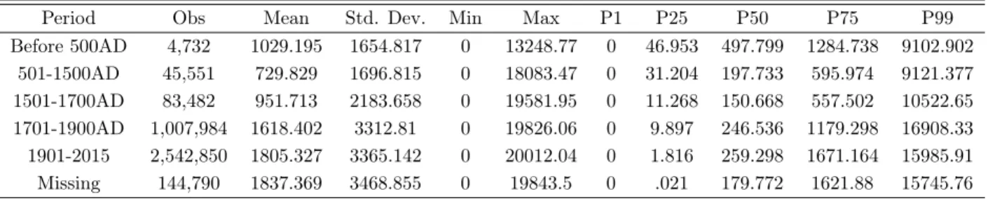
Period Obs Mean Std. Dev. Min Max P1 P25 P50 P75 P99 Before 500AD 4,732 1029.195 1654.817 0 13248.77 0 46.953 497.799 1284.738 9102.902 501-1500AD 45,551 729.829 1696.815 0 18083.47 0 31.204 197.733 595.974 9121.377 1501-1700AD 83,482 951.713 2183.658 0 19581.95 0 11.268 150.668 557.502 10522.65 1701-1900AD 1,007,984 1618.402 3312.81 0 19826.06 0 9.897 246.536 1179.298 16908.33 1901-2015 2,542,850 1805.327 3365.142 0 20012.04 0 1.816 259.298 1671.164 15985.91 Missing 144,790 1837.369 3468.855 0 19843.5 0 .021 179.772 1621.88 15745.76 Table 15: Distance from birth to any identified GeoLink per individual (in km, Full sample, by periods)
Visib. Perc. Obs Mean Std. Dev. Min Max P1 P25 P50 P75 P99
All 2,903,945 1559.643 3199.134 0 20,012.04 0 .092 176.389 1207.587 16,287.4 90 313,248 1970.395 3459.575 0 19,789.02 0 19.559 389.453 1874.146 16,365.76 95 401,799 2286.674 3681.198 0 19,941.56 0 67.235 549.752 2549.724 16640.06 99 175,629 2567.837 3781.461 0 19,936.87 0 145.157 740.887 3337.66 16453.98 99.9 34,768 2573.893 3672.483 0 19,243.99 0 171.841 785.636 3473.262 15,716.43 Table 16: Distance from birth to any identified GeoLink in individual’s life, in km (most visible indi-viduals)
Figure 13: Average distance between birth place and current location
It can be seen that the typical individual leaves his or her birthplace between 10 and 20, and after 20 the median distance of the individual to his or her birthplace is over 200 km.
Trajectories Origin Destination # Mean Percentile Visib. 1 UK USA 35,061 64.5% 2 CAN USA 28,202 60.0% 3 GER USA 15,541 66.5% 4 US CAN 13,816 58.0% 5 UK AUS 13,719 49.6% 6 UK FRA 9,702 67.7% 7 IRE UK 9,636 61.1% 8 USA FRA 8,005 69.1% 9 AUS UK 7,706 64.4% 10 ITA US 7,098 71.5%
Table 17: Most common country-to-country trajectories
3.3 Identified international mobility
One recovers the full addresses, including the country information of all geocodes in the database (current location, places of birth and death when available). The country of origin corresponds to borders in 2015. We round up after the third digit the geocoordinates of all GeoLinks including places of birth and death. We obtain a grand total of 276,677 unique locations identified in the database. Of those, we match a total of 259,109 locations with a country and most of the time a full address, using the command geocode3 and a specific application, Google Maps Geocoding API. We then match these countries to the original locations. Of all non-unique geolinks present in the database, one is able to match 4,859,007 with a country. As for the individual’s database, the U.S. represents the largest share (1,831,479 lines), followed by the UK (821,807 lines), then Germany, Canada, France, Italy, etc. The total number of countries, including overseas territories such as Mayotte or Saint-Pierre et Miquelon, islands such as Turks and Caicos Islands, U.S. Minor Outlands, Guam etc. is 248. Only 35,421 geocodes are returned as “not found” by the Google App. We finally create a variable “move_country” if the country of birth differs from the country of the current geolink, and none of the birth and current countries are missing or “not found”. In the database, 19.7% of identified geolinks with a country have a country of birth different from the country of the individual’s current location.
In time, we obtain a U-shape with a positive and accelerating trend from 1960 to 2015, as Figure14a shows. The right panel, however, shows that this is more due to a composition effect, the “Entertain-ment” category being more internationally mobile and having a growing share in the sample as time goes on. Nevertheless, all categories exhibit a rising fraction of country-to-country mobility.
Figure 14: Country to country mobility
4 Connecting people to cities
In this section, we introduce a new unified database with global historical urban population. We have different data sources covering distinct periods but with different population concepts: some cover urban areas, some other cities defined by administrative boundaries. Most Censuses date back to the beginning of the 19th Century and indeed cover city population but not agglomeration population. To our knowledge no unified database with Census historical data has yet been gathered. We present first the different Census sources identified and collected through scraping and OCR and compile a global historical Census population database.
We then complete the population database with available data from other sources for different periods: 1500-1800 (Urbanisation Hub-Bairoch-Bosker) which covers cities and the surrounding areas when con-tiguous, then 1800-2010 (Lincoln Institute of Land Policy) for the largest cities outside Europe, and finally after 1950 (UN Population database). Figure 1 below illustrates how these different sources, either official or academically certified, complement each other.
Figure 15: Timeline of sources used
After the urban population data was collected, city names were geocoded using the Google Maps API and matched with the trajectories of notable people.
4.1 Data collection
4.1.1 Period 1800-2010: Census records and Lincoln Institute
We collected and assembled detailed and official Census records. Census collections started in the early-to-mid-19th century. Census records are available primarily from National Statistical Institutes and cover a larger number of ‘cities’: 36,541 communes in France, 9,148 communes in Italy, 8,915 urban centers in Canada, and 1,008 incorporated cities in the United States, etc.
In order to obtain historical census data, multiple methods of data extraction were used. When down-loadable digitized census records were not available, web scraping (for 6 countries) and optical character recognition (OCR for 3 countries) helped extract the required data. Certain manipulations on the ex-tracted data were required, such as aggregating city data to urban areas, matching city names across datasets, and combining male/female portions of urban populations. More information on these dif-ferent methods, but also on official links used to access the data, city definitions, dates, number of observations and years available and more are reported in Table18. .
In a few instances, city limits and definitions changed over time, due to land organization differences, evolving urban administrative regions, etc. An example is the UK where data are consistent between 1801 and 1911, but inconsistent with the period 1921-1961. In the longitudinal analyis, we treat these two samples a set of distinct cities (e.g. an unbalanced panel) to avoir dealing with non-comparable datasets. A list including all manipulations performed in the data extraction process is included in the Online appendix. Official census records have been collected for 2 countries in Asia (India and Japan), 11 countries in Europe (Austria, Belgium, Denmark, France, Germany, Italy, Netherlands, Portugal, Russia, Switzerland, United Kingdom), 2 countries in America (Canada and United States) and 2 countries in Oceania (Australia, New Zealand). Information for 65,087 different cities around the world has been gathered. Countries have been chosen both for the primary role they played over the course of history and the availability of official census records for these countries.
To complement the Census dataset over the same period, we use a database compiled by the Lin-coln Institute of Land Policy which provides historical urban population data for 30 major urban agglomerations from 1794 to 2005. The data is reported in intervals of 20 or 25 years and was used to fill gaps of missing data where city limits permitted. This database comprises the following cities sorted by continent and sub-region: Africa (Accra, Algiers, Cairo, Johannesburg, Lagos, Nairobi), Asia (Bangkok, Beijing, Kolkata, Mumbai, Shanghai, Tehran, Tel Aviv), Central America (Guatemala City, Mexico City), Eurasia (Istanbul, Moscow), Europe (Warsaw), Middle East (Jeddah, Kuwait City), South America (Buenos Aires, Santiago, Sao Paulo) and Southeast Asia (Manila). We only used in-formation concerning cities for which we failed to find reliable census data and thus did not consider Lincoln data for Chicago, Los Angeles, Paris, London, Sydney, or Tokyo.
Using Census years (typically every 10 years), we linearly interpolate population for each city in the databse to obtain yearly population and then collapse city population into periods of time of 10 years intervals (e.g. 1801-1810, 1811-1821 etc to 2001-2010).
4.1.2 Backward extension 800AD–1800AD: The Urbanisation Hub-Bairoch-Bosker database To account for city population from 800 to 1800, we used an urban population database compiled initially by Bairoch et al. (1988) and further revised by Bosker et al. (2013). The maximum number of
Con tin en t Cou ntry Cit y De fi niti on Date s Num b er M ax # So ur ce Data Extraction of ye ars of O bs. M eth od Asia Indi a To w n s an d S u b u rb s 1863-1911 7 272 Eng li sh P ar li am en t Excel do w nl oa d or Can ton me nts / Un iv ersit y of Ch ic ago Japan Shi 1873-2010 24 50 Statistics Japan E xcel do wnload Eur op e Austria Comm unes 1869-2001 14 200 Wikipedia (c ross-re fe re nc ed W eb sc rap with Statistik Au stria) Be lgiu m Comm un es 1846-2015 5 571 Statistic s Be lgiu m O CR Denmark Urban Areas & Is lands 1769-2015 72 20 Statis tik B ank en Excel do wnload Fr an ce C om m un es 17 93 -2 00 6 34 36 ,5 41 C as si ni We b sc ra p Ger m an y Gr oß st adt 18 16 -2 01 3 31 76 Wikipedia &D eu ts ch e W eb sc ra p Ve rw al tu n gs ge sc h ic ht e It al y C om m unes 18 42 -2 01 1 16 9, 14 8 St at . B ur ea u of It al y W eb scr ap Netherlands Village/M unicipaliti es 1795-1919 10 2903 Stat. Bureau of the Netherlands Excel do wnload Po rt ug al L oc al id ad es co m m ai s 1864-2011 15 310 National Statistical Excel do wnload de 10 m il ha res ha bi ta nt es Ins ti tut e of P or tug al Russia Urban Cen ter 1750-2001 38 163 P opulstat W eb Scr ap Sw it zer la nd C om m unes 18 50 -1 99 0 15 30 19 St at . B ur ea u of Sw it ze rl and OC R United Kingdom Pr e-1 84 1: Ur ba n C en ter s 1801-1911 12 934 UK Data Arc hiv e / Cam bridge U. Excel do wnload Po st -1 84 1: U rb an A re as / U K C en su s Muni ci pa l B or oug hs 19 21 -1 96 1 4 38 1 V is io n of B ri ta in / Uni ted Ki ng do m C ens us W eb scr ap North America Can ad a Urb an Ce nte rs 1871-1961 11 1,008 Statistic s Can ad a O CR United States Incorp orated Cities 1790-2010 23 8,915 US Census Bureau & P opulstat Excel do wnloa d Ocea ni a Australia Capital cities (8) 1901-2011 96 8 Statistical Bureau of Australia Excel do wnload New Zealand Urban agglomerations 1916-2006 11 568 Statistical Bureau of New Zealand Excel do wnload T ab le 18 : Ce ns us da ta : so ur ce s an d m ai n ch ar ac te ri st ic s
European cities in the revised version of the database amounts to 677 cities in the year 1800. All cities in Bosker at al. (2013) include more than 10,000 inhabitants and are generally defined as urban areas, where “suburbs (faubourgs) surrounding the center” are included. Bosker et al. updated Bairoch’s database by scanning recent literature concerning the major cities covered. In particular, they updated all cities which during a point in history were larger than 60,000 inhabitants. This led to a number of important revisions of population records concerning Muslim cities in medieval Spain but also for the cities of Palermo, Paris, Bruges, and London. Although these revisions decrease the total number of cities covered, the remaining observations are thought to be more reliable.
Bosker et al. (2013) additionally added Middle Eastern and North African cities to Bairoch et al. (1988), which previously only included European cities. This allowed us to obtain historical urban population data on a total of 116 cities coming primarily from the countries of Egypt, Turkey, the former Yugoslavia, Saudi Arabia, Oman, Yemen, Israel, Iraq, Lebanon, Libya, Tunisia, Algeria, and Morocco.4
Using available years (typically every 50 years or 100 years before 1000AD), we linearly interpolate population for each city in the databse to obtain yearly population and then collapse city population into our Time Periods of length of 50 or 25 years intervals (801-850 to 1651-1700, then 1701-1725, 1726-1750, etc.).
4.1.3 Forward extension 1950AD-2010AD: The United Nations database
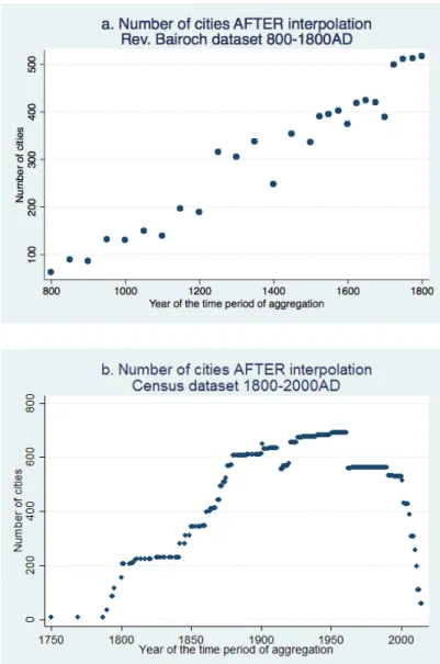
A database provided by the United Nations’ Department of Economic and Social Affairs gives urban agglomeration data from 1950 to 2010 at five year intervals. The definition of an urban agglomeration in this source references an urban area with over 300,000 inhabitants. This database was very useful since the data available from census records decreased steadily starting in the mid-20th century, as seen in Figure16b below. The other advantage of this dataset compared to any other source of information is its worldwide coverage. In all, this database contains population data for 1,692 cities. We collapse the data into ten year intervals: 1951-1960, etc.
Keeping only the largest 50 cities in coutries larger than 300,000 sq. km and the largest 30 cities in other countries (or less if fewer cities where avaialble), we end up with a panel of cities linearly increasing from 800AD to 1800AD (Source: Bairoch-Bosker) and increasing by steps (as larger countries enter the database with a first Census) from 1800 to 1950. See Figure 16b. After 1950, the Census database decreases since the last Census available online varies from country to country (e.g. in the United Kingdom, the database terminates in 1961). We use after 1950 the UN database and its 1,692 cities.
Figure 16: Number of cities by source of data (UH-Bairoch-Bosker ; Census ), only retaining the largest 30/50 cities in each country
4.2 Distances to a large city ; at birth, at death, and in between
From now on, the city database is limited to the top 50 or 30 cities (for which population is available) in each country. We match the GeoLinks to the three nearest cities of this database period by period and only when population is available in that period. We use the geonear command, from geocodes of individuals’ locations and of cities. It also returns distances in kilometers based on geodetic distances, “using a mathematical model of the earth” as specified in the description of the command. Figure 17
shows on the left hand side the cumulative density of distances of the third three cities. The Bairoch database covers well the individual’s locations: over the period 800-1800AD, 60 percents of GeoLinks are located within a radius of 50 kilometers around a city in the database. Another 30% of GeoLinks
are within 50 kilometers of a second nearest city, and 17% are within 50 kilometers of the third nearest city. Similarly, 50% of individuals over the period 1800-1939 are within 50 kilometers of the closest city. Finally, the last period of the sample, based on the UN database, is the best matched: 80% of GeoLinks are within 50 kilometers of the closest city. On the right part of the graph, we represent the cumulative distance to the closest city by occupation. They do not differ much for the Census and the UN database of cities, but differ according to occupation over the period 800-1800, Academics and Entertainment (Arts, Literature and Media only over this period) being significantly more likely to be close to a big city.
Figure 17: Distances between individual’s locations and nearest cities in the three samples: Bairoch-Bosker ; Census ; United Nation Database
4.3 Facts on city rank, visibility and occupations
The last observations lead to a study of the relations between city size (or rank) and occupation and visibility. It can be seen from Figure 18(left panels) that there is no systematic correlation between city rank in a country and the degree of visibility (in logs). For the top four cities, it turns out that the c.d.f. of log visibility are quite close to each other and the lowest c.d.f. is that of the first city and
this is true over the three sub-samples (800-1800AD, 1800-1939AD and post 1950). For instance, in the sample of Census data (1800-1939), the correlation coefficient between log visibility and city ranks from 1 to 50 is -0.08 and -0.07 if limited to the first 4 cities.
When the rank of the city is calculated for all countries, as in the right part of the Figure, things are different (e.g. over the period 1800-1939AD London, New York, Paris, Beijing are ranked as first cities in the world, etc.), the pattern is different. Individuals in the first city have higher visibility, and have lower visibility in the second, fourth, and then third cities in the world. The correlation coefficient between that rank from 1 to 4 is now positive, equal to 0.17. However, the correlation between city rank and visibility of individuals is negative again in the post 1950 period where the biggest cities in the world are in located in developing countries (bottom right chart).
Figure 18: Links between city rank and visibility. Left charts: ranking within countries ; right charts: wolrd ranking. Top: Bairoch city dataset (800-1800AD); Middle: Census city datasets ( 1800-1939AD) ; bottom : UN city dataset (1950-2000AD)