HAL Id: hal-01322017
https://hal.archives-ouvertes.fr/hal-01322017
Submitted on 26 May 2016
HAL is a multi-disciplinary open access
archive for the deposit and dissemination of
sci-entific research documents, whether they are
pub-lished or not. The documents may come from
teaching and research institutions in France or
abroad, or from public or private research centers.
L’archive ouverte pluridisciplinaire HAL, est
destinée au dépôt et à la diffusion de documents
scientifiques de niveau recherche, publiés ou non,
émanant des établissements d’enseignement et de
recherche français ou étrangers, des laboratoires
publics ou privés.
Distributed under a Creative Commons Attribution - NonCommercial - NoDerivatives| 4.0
International License
Plane Wave Imaging for ultrasonic non-destructive
testing: Generalization to multimodal imaging
Léonard Le Jeune, Sébastien Robert, Eduardo Lopez Villaverde, Claire Prada
To cite this version:
Léonard Le Jeune, Sébastien Robert, Eduardo Lopez Villaverde, Claire Prada. Plane Wave Imaging
for ultrasonic non-destructive testing: Generalization to multimodal imaging. Ultrasonics, Elsevier,
2016, 64, pp.128-138. �10.1016/j.ultras.2015.08.008�. �hal-01322017�
Plane Wave Imaging for Ultrasonic Non-Destructive Testing:
Generalization to Multimodal Imaging
L´eonard LE JEUNE∗, S´ebastien ROBERT, Eduardo LOPEZ VILLAVERDE
CEA, LIST, Gif-sur-Yvette, F-91191, France
Claire PRADA
Institut Langevin, 1 rue Jussieu, 75238 Paris Cedex 05, France
Abstract
This paper describes a new ultrasonic array imaging method for Non-Destructive Testing (NDT) which is derived from the medical Plane Wave Imaging (PWI) technique. The objective is to perform fast ultrasound imaging with high image quality. The approach is to transmit plane waves at several angles and to record the back-scattered signals with all the array elements. Focusing in receive is then achieved by coherent summations of the signals in every point of a region of interest. The medical PWI is generalized to immersion setups where water acts as a coupling medium and to multimodal (direct, half-skip modes) imaging in order to detect different types of defects (inclusions, porosities, cracks). This method is compared to the Total Focusing Method (TFM) which is the reference imaging technique in NDT. First, the two post-processing algorithms are described. Then experimental results with the array probe either in contact or in immersion are presented. A good agreement between the TFM and the PWI is observed, with three to ten times less transmissions required for the PWI.
Keywords: Transducer array; Non-destructive testing; Ultrasonic imaging; Defect characterization
1. Introduction
Ultrasonic transducer arrays are more and more used for industrial Non-Destructive Testing (NDT). Compared to single element transducers, they are much more versatile as they allow different inspection modes (plane waves, steered angle beams, focused beams) and can be used to produce images (focused Bscans, focused Sscans [1, 2]) at a single position. In array imaging, one of the best method is the Synthetic Transmit Aperture (STA [3, 4]), also called Total Focusing Method (TFM) in the NDT field [5]. This method is based on the post-processing of the full array response matrix K(t) [6], called Full Matrix Capture (FMC) in NDT. For a N element transducer, the FMC consists in recording the N × N inter-element impulse responses kij(t), defined as the signal received by element j when an electric pulse is applied to element i. The TFM allows to focus on every point of the image area while, in the focused Sscans and focused Bscans modes, the image is constructed line by line and by focusing at a given depth. This technique has several advantages compared the other imaging methods (focused Sscans, focused Bscans). The main advantage of the TFM is the image quality as the focusing and spatial resolution are optimal everywhere in the region of interest. Another benefit is the possibility of applying different imaging modes to the same array response matrix, depending on the nature of the defects [7–9]. For example, images can be made using half-skip paths, including a reflection on the back-wall before interacting with the defect, to image crack-type defects.
∗Corresponding author
Finally, unlike in focused Bscan, the TFM image area can be larger than the probe and is not related to the number of shots, contrarily to focused Sscan images. However, the TFM technique has two main drawbacks. The first one is a limited acoustic power sent into the medium due to the use of only one element per emission. This results in a degradation of the signal to noise ratio (SNR) and can be troublesome in the case of attenuating materials and random noise. Moreover, controls looking for crack-type defects are made typically around 45◦, thus the image is not centered under the probe. In this situation, the cylindrical wave emitted by an element, radiating mainly perpendicularly to the transducer plan, is not the most fitted type. In some cases, this is highlighted by the existence of non-physical indications, also called image artifacts, that may lead to misinterpretations [10, 11]. The second drawback is the frame-rate limit due to the number of transmissions (N ) and the storage and processing of the N × N signals. Techniques exist to reduce the number of signals to be processed, like the Sparse Matrix Capture (SMC) that uses a few elements in transmission, compensating the loss of acoustic power by creating virtual sources [12–15].
In order to improve the frame-rate and increase the acoustic power sent into the medium, the Plane Wave Imaging (PWI [16–18]), recently developed in the medical field, seems to be very promising for NDT inspections. The principle is to transmit plane ultrasonic wave-fronts at different angles in the medium. For each plane wave transmission, the PWI image is reconstructed line by line by dynamically focusing in receive mode at different depths with a subset of several adjacent receivers. The final image is then obtained by summing the images obtained for every angle. This method has several advantages in medical imaging. The main advantage is a high image quality obtained with a few ultrasonic shots (typically 10 to 30 for a 128 elements probe). Furthermore, as all the probe elements are excited together, the acoustic power sent in the medium is high. Thus, this method is less sensitive to attenuation and random noise than the TFM. The main drawback is that the image size is limited by the probe aperture. The number of lines in the image depends on the number of elements, and a classical NDT inspection uses transducers with 32 to 64 elements. Thus the number of elements and, therefore, the image size are too small to perform accurate inspections. Moreover, the PWI used in the medical field can not image crack-type defects. This is due to the fact that subsets of elements are used in reception, while crack-type defects imaging requires reception on all the probe elements to use half-skip modes.
In this paper, we present a technique that combines the advantages of the PWI and the TFM. The main objective is to prove that high quality images can be obtained by the transmissions of plane waves. The second goal is to explore the possibility to reduce the number of transmissions and to limit imaging artifacts due to mode conversions. The medical PWI is generalized by taking into account the refraction on a plane interface, the bulk wave polarizations (longitudinal: L, transverse: T ) and the paths including interactions with the back-wall (half-skip modes). In transmission, plane waves are emitted at different angles and the backscattered signals are recorded by the elements. Thus creating a Q× N matrix where Q is the number of plane waves transmitted and N is the number of elements in the probe. This matrix is then post-processed to perform beamforming in transmit and receive modes. This method will allow multi-modal PWI imaging (direct and half-skip modes) with high acoustic power sent into the inspected material and low acquisition time. In the first section, the theoretical backgrounds of the multi-modal TFM and PWI methods are presented. The second section presents and compares experimental results obtained with the two methods for different types of defects.
2. Theoretical background
This section describes the theoretical backgrounds of the Total Focusing Method (TFM) and Plane Wave Imaging (PWI) techniques. For a general description, we consider an immersion configuration, where the array and the specimen are immersed in water. First, they are derived for simple round-trip, also called direct modes. In these modes, the wave goes from the transmitter to the focusing point and back to the receiver. Then, they are generalized to half-skip mode reconstructions in which the wave goes from the transmitter to the focusing point after reflection on the back-wall, and back to the receiver. The direct modes are useful to image volumetric flaws (holes, porosities, inclusions) while half-skip modes are used to enhance the characterization of crack-type defects.
2.1. TFM Algorithm
The TFM imaging technique is applied to the full array response matrix K(t). This matrix contains the N× N inter-element impulse responses kij(t), corresponding to the signal received by element j when an electric pulse is applied to element i. The TFM consists in coherently summing all the analytical signals sij(t) = kij(t) + jH(kij(t)), where H is the Hilbert’s transform [5]. Thus, the ultrasonic beam is focused on every point of a region of interest (ROI). Considering a point P in the ROI, the amplitude A(P ) at this point is given by:
A(P ) =| N X i=1 N X j=1 sij(tPi + tPj)|, (1) where tP
i (resp. tPj) is the time of flight between transmitter i (resp. receiver j) and point P . The difficulty of the method lies in the determination of the times of flight where the refraction at the interface between the coupling medium (water) and the inspected material (steel) has to be taken into account.
2.1.1. Imaging with Direct Modes
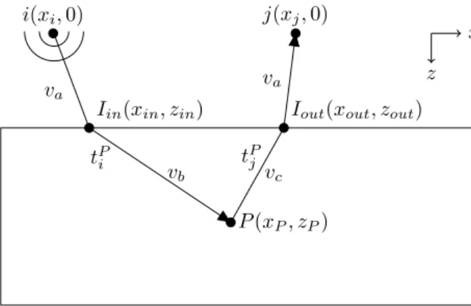
In direct mode, the ultrasonic wave propagates from a transmitter to the focusing point and back to a receiver, through the surface (Fig. 1).
x z va vb vc va tPi t P j i(xi, 0) P (xP, zP) Iin(xin, zin) j(xj, 0)
Iout(xout, zout)
Figure 1: Illustrations of the paths followed by a wave in direct mode TFM imaging. The cylindrical wave transmitted by element i propagates to the focus point P through the surface at Iin, and back to receiver j through the surface at Iout.
For the incident path, the wave goes from the transmitter i(xi, 0) to the impact point Iin(xin, zin) on the surface at the sound velocity in water va. Then it propagates from Iinto the focusing point P (xP, zP) with the velocity vb, which can be the velocity of the longitudinal (vL) or transverse (vT) waves, depending on the type of wave used. The outgoing path follows the same pattern, the wave going from the focusing point P to the impact point Iout(xout, zout) with the celerity vc (vL or vT) and then from Iout to j(xj, 0) with the sound speed va. The following demonstration focus on the incident wave because, for a pair element/focus point, the paths in transmission and in reception are identical. The time of flight corresponding to the incident path is given by:
tPi =
p(xin− xi)2+ zin2
va +
p(xP− xin)2+ (zP− zin)2
vb . (2)
The Fermat’s principle states that the physical path corresponds to the minimum time of flight, which can be estimated by finding the zeros of the first derivative of tP
i with respect to xin. This is equivalent to solve the Snell-Descartes law of refraction:
vb va (xin− xi) p(xin− xi)2+ zin2 −p(x (xP− xin) P− xin)2+ (zP − zin)2 = 0. (3)
For a plane interface, by squaring Eq. 3, an analytical solution can be obtained by Ferrari’s method [19]. A more general approach, also available for more complex surfaces, is to solve Eq. 3 using an iterative technique like the Newton-Raphson method. This technique is used to find the roots of a real-valued function f (x) like Eq. 3. For a one variable problem, the Newton-Raphson method is expressed as follows:
x(k+1)= x(k)− f (x (k))
f0(x(k)), (4)
where k is the iteration order and f (x), f0(x) are the function and its first derivative. In the present configuration, with V = vb/va, the function and its first derivative can be expressed by:
f (xin) = V (xin− xi) p(xin− xi)2+ z2in − (xP− xin) p(xP − xin)2+ (zP− zin)2 f0(x in) = V z2 in [(xin− xi)2+ zin2] 3 2 + (zP− zin) 2 [(xP − xin)2+ (zP− zin)2] 3 2 . (5)
The impact point of abscissa xin is necessarily situated between the transmitter and the focusing point abscissas (i.e. xin < xi < xP). Moreover, the velocity in water being significantly lower than the ones in the inspected medium, the impact point is located closer to the emitter abscissa xi. Therefore, the initialization value x0 is chosen at the transmitter abscissa x
i. Once the impact point coordinates are known, the distance between the element and the focus point can be calculated geometrically thus giving the corresponding travel time (Eq. 3). Finally for every transmitter/receiver pair and every point in the ROI, the amplitudes associated to the computed times of flight are added following Eq. 1, to form the TFM image. Note that for reconstructions without mode conversion (LL, T T ), the velocities of the incident and backscattered waves in the material are identical. Thus, N times of flight have to be computed to focus on a point. For reconstructions with mode conversions (LT , T L), the speeds of the incident and backscattered waves in the material are different (vb6= vc). Therefore, for every point P in the ROI, N + N times of flight have to be determined to focus on a point.
2.1.2. Imaging with Half-skip Modes
In half-skip modes, due to the reflection on the component back-wall, the paths in transmission and reception are different. Therefore, there is necessarily N + N times of flight to compute and three impact points have to be determined: two on the surface (incident and backscattered waves) and one on the back-wall (incident wave).
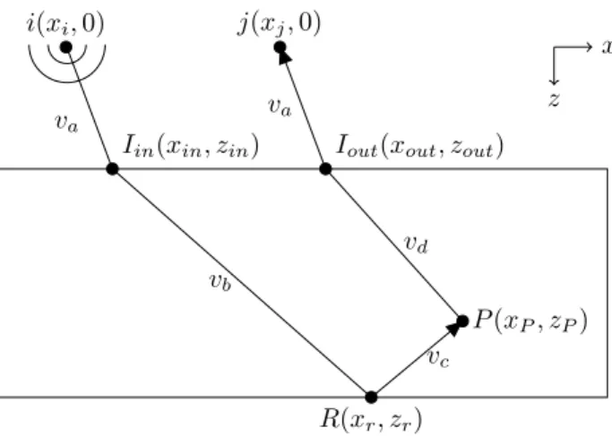
As illustrated in Fig. 2, the paths followed by the backscattered wave in half-skip and direct modes are identical. Thus, the times of flight for the backscattered waves can be obtained thanks to Eq. 2 and the method described in 2.1.1. For the incident wave, with the notations in Fig. 2, the problem can be written as: f1(xin, xr) = vb(xin− xi)p(xr− xin)2+ (zr− zin)2 − va(xr− xin) q (xin− xi)2+ zin2 f2(xin, xr) = vc(xr− xin) q (xf− xr)2+ (zf− zr)2 − vb(xP− xr)p(xr− xin)2+ (zr− zin)2 , (6)
where (xi, zi) are the transmitter i coordinates, (xin, zin) the impact point Iincoordinates on the surface, (xr, zr) the impact point R coordinates on the back-wall and (xP, zP) the focus point P coordinates. All
x z va vb vc vd va i(xi, 0) P (xP, zP) R(xr, zr) Iin(xin, zin) j(xj, 0)
Iout(xout, zout)
Figure 2: Illustration of the paths followed by the wave in half-skip mode TFM imaging. The cylindrical wave transmitted by element i propagates to the focus point P after refraction at the surface at Iinand reflection on the back-wall at R, and goes
back to receiver j through the surface at Iout.
the parameters are known except for xinand xrand the Newton-Raphson algorithm can be used again. Its general form is given by:
X(k+1)= X(k)− J−1f (X(k))f (X(k)), (7) where X(k)= (x(k)
in, x (k)
r ) is the vector of coordinates to be determined with k the iteration order, f = (f1, f2) is defined by Eq. 6 and must vanish and J−1f is the inverse of the Jacobian matrix of f expressed by:
J−1f = 1 det Jf ∂f2 ∂xr − ∂f1 ∂xr −∂x∂f2 in ∂f1 ∂xin . (8)
By solving this system, the different impact points can be determined and provide the ultrasonic path and the associated time of flight:
tP i = p(xin− xi)2+ z2in va +p(xr− xin) 2+ (z r− zin)2 vb +p(xP − xr) 2+ (z P− zr)2 vc . (9) 2.2. PWI Algorithm
The principle of PWI is to emit a set of Q plane waves at Q angles and to record the back-scattered signals on every element, thus creating a Q× N matrix M(t). In medical PWI, for every angle, the image is constructed line by line by applying delay laws and summations to the raw RF signals to focus on points at a few different depths. The sub-aperture used to obtained a line is determined by the F -number: F = zP/L, where zPis the focal point depth and L the sub-aperture width. Then, the images obtained for each angle are summed-up to form the final image. As underlined in the introduction, the PWI from the medical imaging can be used in NDT but it needs to be adapted to the NDT context. The method has to be generalized to immersion configurations, where refraction at the interface between the coupling medium and the specimen must be taken into account, and allows more complex reconstruction modes (half-skip modes). Here, the proposed method relies on an algorithm that allows to focus on every point of a ROI. As the ultrasonic beam
is focused on every point of the ROI, this will improve the PWI image quality. Furthermore, this allows to obtain images outside the probe aperture and to perform half-skip modes, including mode conversions (LT T , T T L,. . . ). With this modified PWI, for a set of Q angles and a point P in the ROI, the amplitude at this point is obtained by summing coherently all the sqj(t) given by the Hilbert’s transform of the mqj(t) component of M(t): A(P ) =| Q X q=1 N X j=1 sqj(tPq + tPj)|, (10) where tP
q is the time spent by the plane wave at angle q to reach the focusing point P , tPj is the time of flight between the focusing point P and the receiving element j. Note that in Eq. 10, all the N elements are used in reception contrarily to the medical PWI. In transmission, as the plane wave is emitted at a defined angle, the impact point at the interface between the two media can be calculated geometrically, thus making it easier to compute. However, in reception, the impact point has to be calculated as previously in the TFM method, with the Newton-Raphson algorithm (because the backscattered wave is cylindrical).
2.2.1. Imaging with Direct modes
x z va vb vd va αq βq P (xP, zP) Iin(xin, zin) j(xj, 0)
Iout(xout, zout)
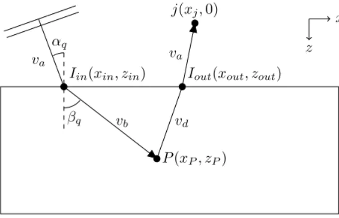
Figure 3: Illustration of the paths followed by the wave in direct mode PWI imaging. The plane wave transmitted by a transducer parallel to the interface propagates to the focus point P after refraction at the surface at Iin and goes back to
receiver j through the surface at Iout.
Contrarily to the TFM method, where transmitted waves propagate in all the directions, the plane wave is transmitted in the water with a known angle αq. Therefore, the impact point on the surface can be computed geometrically:
xin= zintan αq, (11)
with αq = sin−1(va/vbsin βq). This allows to calculate the time of flight for the incident wave from the transducer to the focusing point P :
tPq = xinsin αq+ zincos αq va +(xP− xin) sin βq+ (zP− zin) cos βq vb . (12)
The time of flight from the focusing point to a receiver j (tP
j) can be calculated as in 2.1.1. In direct modes, whatever the imaging mode (with or without mode conversions), there are N + Q computed times of flight to focus on a point.
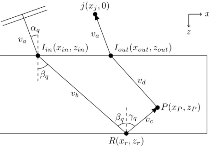
x z va vb vc vd va αq βq βq γq P (xP, zP) R(xr, zr) Iin(xin, zin) j(xj, 0)
Iout(xout, zout)
Figure 4: Illustration of the paths followed by the wave in half-skip mode PWI imaging. The plane wave transmitted by a transducer parallel to the interface propagates to the focus point P after refraction at the surface at Iinand reflection on the
back-wall at R, and goes back to receiver j through the surface at Iout.
2.2.2. Imaging with Half-skip Modes In half-skip modes, the times of flight tP
j from the focusing point to a receiver can be obtained as in 2.1.1. For the incident wave, there are two impact points to be determined (Iin, R). The impact point Iin on the surface can be found thanks to Eq.11 and, as the component back-wall depth zris known and with the notations in Fig. 4, the impact point coordinate xron the back-wall can be written as:
xr= xP − (zr− zP) tan γq, (13)
with γq = sin−1(vc/vbsin βq). Once the impact point R coordinates are known, the path followed by the incident plane wave and the associated times of flight can be computed:
tPq = xinsin αq+ zincos αq va +(xr− xin) sin βq+ (zr− zin) cos βq vb +p(xr− xP) 2+ (z r− zP)2 vc . (14)
For these types of modes, the number of times of flight to compute stays the same than for the direct modes (N + Q). Therefore, in direct modes without mode conversions, compared to the TFM method, the number of transmissions of the PWI is reduced (N → Q) but the number of computed times of flight is higher (N → N + Q). However, in direct modes with mode conversion or in half-skip modes, as Q < N, the number of transmissions and of computed times of flight are reduced (N + N→ N + Q).
2.3. Effective Area
As seen in the previous subsections, the PWI algorithm requires less operations than the TFM, which reduces computation times. Moreover, as plane waves are spatially limited, an effective area can be defined for each transmission to apply the algorithm only for the points insonified by the incident wave. This is especially noticeable when the image area is larger than the probe.
The width of the effective area is given by L cos β, where L is the probe aperture and β the transmission angle. Thus when the transmission angle increases, the effective zone width decreases. The use of an effective area limits the effects of the diffraction by the transducer edges or the grating lobes and reduces the number of computation points.
Effective area
Image area β
L L cosβ
Figure 5: Effective area for an arbitrary angle β. The effective area is smaller than the image area (red) and decreases when the angle increases.
3. Simulated and Experimental Results
The imaging methods presented in Section 2 have been compared experimentally. The acquisitions have been performed on two steel mock-ups containing artificial defects. The first one contains 2 mm diameter holes located at different depths. This specimen is used to illustrate the direct mode imaging. The second one contains a 10 mm height notch to illustrate the half-skip mode imaging. The probe used in the direct mode experiment is a 128 elements linear array (2 MHz central frequency, 0.8 mm pitch) manufactured by Imasonic. For the half-skip mode experiment, a 64 element probe with the same characteristics has been used. The data acquisitions have been carried out with a M2M MultiX system.
3.1. Imaging Algorithms Comparison
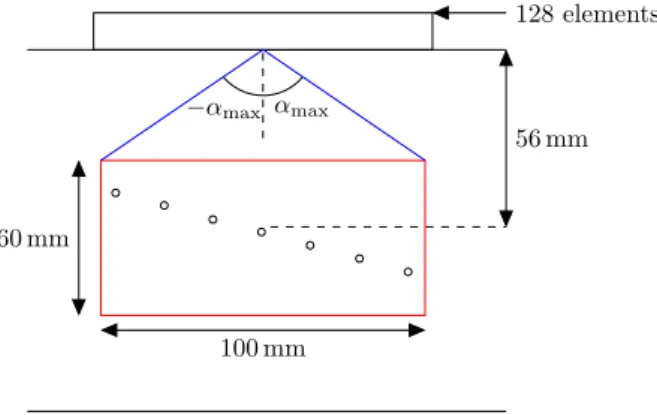
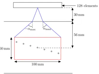
First, to evaluate the performance of the two algorithms, PWI and TFM were applied to the same set of FMC data recorded with a probe in contact with a steel block (Fig. 6). The image area is 100 mm by 60 mm and covers the probe aperture. It is centered on the central hole located at 56 mm depth.
128 elements 56 mm 60 mm 100 mm αmax −αmax
Figure 6: Schematic representation of the inspection setup. The 128 elements probe is placed in contact with the component. Artificial defects (2 mm diameter holes) are included in the steel block, 7 of them being in the image area (red). The blue lines represent the central ray of the extreme transmission angles (αmax± 60◦).
To calculate PWI images, plane waves were synthetized from the K(t) matrix. This was achieved by processing the K(t) matrix in the frequency domain. The N×1 vector Mβ(ω), containing the backscattered waves for a plane wave transmission with an angle β, is given by the relationship Eq. 15:
Mβ(ω) = K(ω) exp(−jωτβ), (15)
where τβ is a N × 1 vector (N: number of elements) of the appropriate delays τβ = (nd sin β)/v − min[(nd sin β)/v], with n the element number (1 < n < N ) and d the probe pitch. Then, the K(t) matrix in the temporal domain is obtained by an Inverse Fourier Transform. The “central ray”(blue lines in Fig 6) of the maximum angles are passing by the corner of the ROI. This guarantee that the synthetised sector scan entirely covers the image area and that every point in the ROI is correctly insonified. In this case, the sector scan is from−60◦ to 60◦ with 1◦ steps. Thus, the number of transmissions is similar for the FMC (128) and the PWI (121). Images are obtained using the LL mode (longitudinal waves back and forth).
−50 −30 −10
10
30
50
40
60
80
X (mm)
Z
(mm)
−60 −50 −40 −30 −20 −10 0 dB (a)−50 −30 −10
10
30
50
40
60
80
X (mm)
Z
(mm)
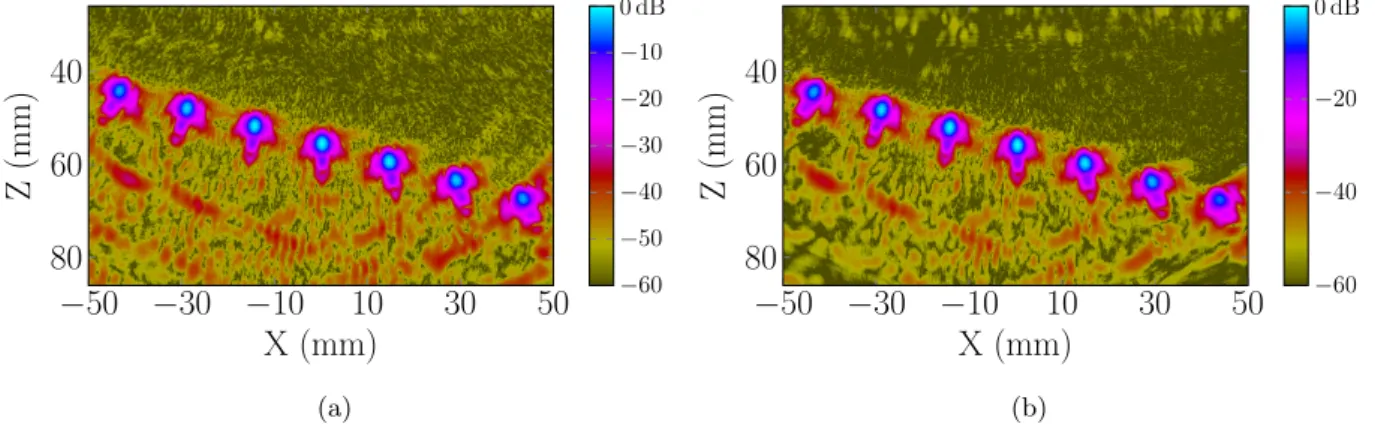
−60 −40 −20 0 dB (b)Figure 7: Experimental images obtained by applying both the TFM (a) and PWI (b) algorithms to the same set of FMC data.
The images displayed in Fig. 7 are very similar and can be separated into two regions characterized by different types of noise: the first region above the defect where noise is mainly incoherent; the second one, below the defect where noise corresponds to artifacts due to the imaging algorithms. It can be noticed that the PWI algorithm (Fig.7b) does not increase incoherent noise in the upper part of the image and that artifacts in the lower part are slightly reduced.
Now that we have verified that the PWI and the TFM provide similar images for similar number of transmissions, we focus on the acquisition process, in order to limit the number of transmissions without degrading the image quality.
3.2. Influence of the Transmission Angular Step on the PWI
In this section, acquisitions performed in contact and in immersion, are used to compare the TFM and PWI methods (acquisition and imaging algorithm). First, the PWI image is obtained using all the transmitted angles with a 1◦ step. Then, the influence of the angular step of the PWI is studied and a compromise between the Signal to Noise Ratio (SNR) and the number of plane waves is deduced.
3.2.1. Acquisition Gain Selection
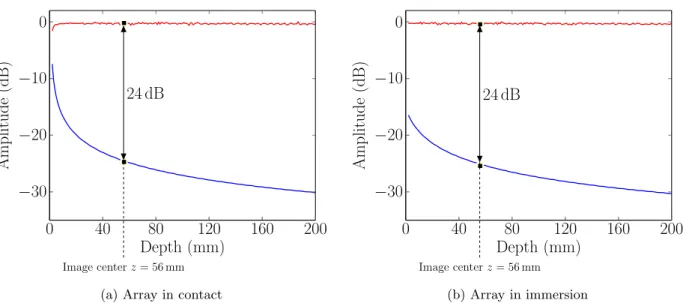
In a FMC, one element at a time is firing whereas, in a PWI acquisition, all the elements are excited simultaneously and transmit plane waves with higher amplitudes. To compare the performance of the two methods with all things being equal, this amplitude difference must be compensated by increasing the acquisition gain for the FMC. To estimate the required gain difference, the field radiated by an element emitting a cylindrical wave and by an array transmitting a plane wave at 0◦was calculated using the CIVA software [8]. In Fig. 8, the axial amplitude along the depth z are compared in the case of an array in contact (Fig. 6) and in the case of immersion (Fig. 14). Then, the axial amplitudes along the depth z are measured.
0
40
80
120
160
200
−30
−20
−10
0
Depth (mm)
Amplitude
(dB)
24 dB
Image center z = 56 mm (a) Array in contact0
40
80
120
160
200
−30
−20
−10
0
Depth (mm)
Amplitude
(dB)
24 dB
Image center z = 56 mm (b) Array in immersionFigure 8: Axial field amplitude for a cylindrical wave (–), and for a plane wave at 0◦(–) for (a) a contact phased-array ; (b)
an array in immersion.
As expected, the cylindrical wave field decreases as 1/√z because of the cylindrical spreading, whereas the plane wave field is constant. At the imaging depth (around 56 mm) the field amplitudes differ by approximately 24 dB. In consequence, in the following experiments, the gain will be fixed 24 dB higher for the FMC than for the PWI acquisition.
3.2.2. Case of a Transducer in Contact with the Specimen
To compare the TFM imaging and the PWI in direct mode, a FMC and a sector scan acquisition have been performed for the same probe position. The transducer is placed in contact with the steel mock-up (Fig. 6). The sector scan is defined from−60◦ to 60◦ with 1◦ step. Thus, the number of transmissions is similar for the TFM (128) and the PWI (121).
−50 −30 −10
10
30
50
40
60
80
X (mm)
Z
(mm)
−50 −40 −30 −20 −10 0 dB (a) TFM−50 −30 −10
10
30
50
40
60
80
X (mm)
Z
(mm)
−50 −40 −30 −20 −10 0 dB (b) PWI: −60◦ to 60◦, 1◦step Figure 9: Experimental images obtained with the (a) TFM (128 transmissions). (b) PWI (121 transmissions).The images displayed in Fig. 9a and 9b prove that the two methods give very similar results. No noise above−50 dB is visible in the upper part of the images but imaging artifacts are present in the lower part below−35 dB. The positions, shapes and amplitudes of the defect echoes are identical.
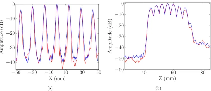
Fig. 10 displays the maximum of the projection along the X direction, also called X-echodynamic curve. We can observe that the defect localization and the amplitudes are similar for the two methods. The lateral
−50
−30
−10
10
30
50
−40
−30
−20
−10
0
X (mm)
Amplitude
(dB)
(a)40
60
80
−60
−50
−40
−30
−20
−10
0
Z (mm)
Amplitude
(dB)
(b)Figure 10: Maximum of the projection of the amplitude along the (a) X direction. (b) Z direction. Red: PWI (−60◦to 60◦, 1◦step), blue: TFM.
resolutions at−20 dB are identical (≈ 4.5 mm). In the images, the noise level of the PWI is slightly lower (≈ 2 dB) than that of the TFM in the upper part. These images show that the TFM and the PWI provide similar results when the number of transmissions is equivalent.
Influence of the angular step on the SNR. An advantage of the PWI is that all elements are used to transmit a plane wave, thus more energy is emitted in the material. Therefore, an equivalent image quality but with fewer transmissions can be expected. Figure 11 shows the signal to noise ratio (SNR) variation as function of the angular step between two consecutive plane waves. The angular range is fixed ([−60◦;−60◦]) and covers all the image area. Then, the angular step is increased from 1◦ (i.e. 121 plane waves) to 60◦ (i.e. 3 plane waves). The SNR is measured by taking the maximum amplitude in an image area around the three central holes, from which the defect echoes have been removed.
0
20
40
60
20
25
30
35
Angular step (
◦)
SNR
(dB)
Figure 11: SNR for the central defect plotted as function of the angular step between two consecutive plane waves.
As expected, the SNR decreases when the angular step increases. The SNR stays approximately con-stant for angular steps from 1◦ to 5◦. This is consistent with the results from Montaldo et al. [16] which
demonstrate that about 40 plane waves are needed to obtain the same contrast value for the PWI and their optimal multifocus method.
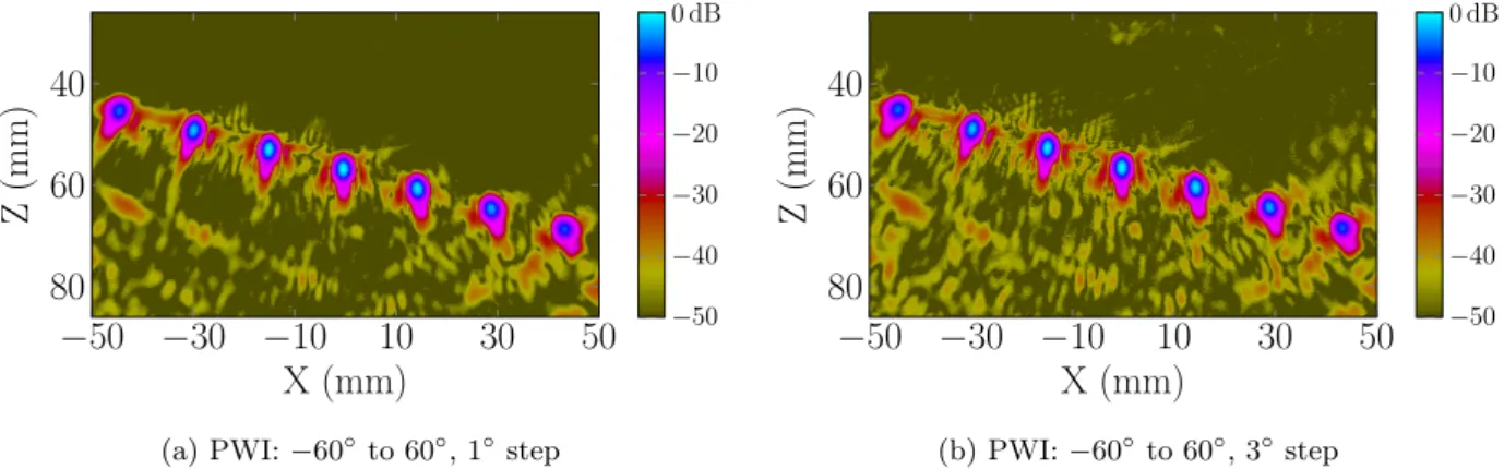
To confirm that the same image quality can be obtained with fewer transmissions, an image is constructed using the full angular sector (−60◦;−60◦) but with 3◦ step between two consecutive plane waves. This corresponds to the transmission of 41 plane waves.
−50 −30 −10
10
30
50
40
60
80
X (mm)
Z
(mm)
−50 −40 −30 −20 −10 0 dB(a) PWI: −60◦to 60◦, 1◦step
−50 −30 −10
10
30
50
40
60
80
X (mm)
Z
(mm)
−50 −40 −30 −20 −10 0 dB (b) PWI: −60◦ to 60◦, 3◦step Figure 12: Experimental images obtained with the (a) PWI (121 transmissions). (b) PWI (41 transmissions).The results presented in Fig. 12 demonstrate that the image obtained with the PWI with 121 plane waves (−60◦ to 60◦, 1◦ steps) and the PWI with 41 plane waves (−60◦ to 60◦, 3◦ steps) are similar. No noise is visible in the upper part of the image and reconstruction noise is present in the lower part. There are a few more artifacts with 3◦ steps but the noise level remains around−50 dB.
−50
−30
−10
10
30
50
−40
−30
−20
−10
0
X (mm)
Amplitude
(dB)
(a)40
60
80
−60
−50
−40
−30
−20
−10
0
Z (mm)
Amplitude
(dB)
(b)Figure 13: Maximum of the projection of the amplitude along the (a) X direction. (b) Z direction. Red: PWI (−60◦to 60◦, 3◦step), blue: PWI (−60◦to 60◦, 1◦step).
These observations are confirmed by Fig. 13 in which noise levels are identical in the X directions (Fig. 13a), whereas for 3◦steps PWI, the noise level is increased by 3◦ to 4◦ in the upper part of the image (Fig. 13b). The chose angular step does not degrade the echo amplitudes and the defect localization is not hampered (Fig. 13a).
128 elements 30 mm 56 mm 60 mm 100 mm αmax −αmax
Figure 14: Schematic representation of the inspection setup. The 128 elements probe is placed in immersion with 30 mm between the probe and the surface. Artificial defects (2 mm diameter holes) are included in the steel block, 7 of them being in the image area (red). The blue lines represent the central ray of the extreme transmission angles (αmax= ±60◦).
3.2.3. Case of a Transducer in Immersion
In this control configuration, the distance between the array and the surface is 30 mm with water acting as a coupling medium (Fig. 14). This ensures that no surface echo will interfere with the defect echoes. The image area is a 100 mm by 60 mm zone that covered the width of the probe and is centered on the central hole at 56 mm depth. Image are made using the LL mode (longitudinal waves back and forth).
−50 −30 −10
10
30
50
40
60
80
X (mm)
Z
(mm)
−50 −40 −30 −20 −10 0 dB (a) TFM−50 −30 −10
10
30
50
40
60
80
X (mm)
Z
(mm)
−50 −40 −30 −20 −10 0 dB (b) PWI: −60◦ to 60◦, 1◦step Figure 15: Experimental images obtained with the (a) TFM (128 transmissions). (b) PWI (121 transmissions).The images obtained with the TFM and the PWI are displayed in Fig 15 and show similar results. There is slightly more noise than in Fig. 9 but the SNR is still below−45 dB. Random noise in the upper part of the images and artifacts in the lower part are present. This is illustrated in Fig. 16b where the curves are very similar. Like for the contact setup, the amplitudes and defects localization are the same for the two methods (Fig. 16a).
Influence of the angular step on the SNR. As for the contact configuration, we study the influence of the angular step on the SNR. The SNR is measured in the same manner than in the previous subsection (3.2.2). As in 3.2.2, the SNR decreases when the angular step increases (Fig. 17). From 1◦ to 4◦, it remains roughly the same and it can be concluded that approximately 40 plane waves have to be transmitted to get the optimal SNR. The images obtained with the PWI using 121 transmissions (−60◦ to 60◦, 1◦ steps) and 41 transmissions (−60◦to 60◦, 3◦ steps) are presented in Fig. 18.
−50
−30
−10
10
30
50
−40
−30
−20
−10
0
X(mm)
Amplitude
(dB)
(a)40
60
80
−50
−40
−30
−20
−10
0
Z (mm)
Amplitude
(dB)
(b)Figure 16: Maximum of the projection of the amplitude along the (a) X direction. (b) Z direction. Red: PWI (−60◦to 60◦,
1◦step), blue: TFM.
Noise in the upper part of the image is slightly higher with 3◦steps (Fig.18b and Fig. 19b) than with 1◦ steps (Fig. 18a and Fig. 19b). Imaging artifacts in the lower part are a little more noticeable with the 3◦ step but they are below−45 dB.
0
20
40
60
24
28
32
Angular step (
◦)
SNR
(dB)
Figure 17: SNR for the central defect as function of the angular step between two consecutive plane waves.
−50 −30 −10
10
30
50
40
60
80
X (mm)
Z
(mm)
−50 −40 −30 −20 −10 0 dB(a) PWI: −60◦to 60◦, 1◦step
−50 −30 −10
10
30
50
40
60
80
X (mm)
Z
(mm)
−50 −40 −30 −20 −10 0 dB (b) PWI: −60◦ to 60◦, 3◦step Figure 18: Experimental images obtained with the (a) PWI (121 transmissions). (b) PWI (41 transmissions).−50
−30
−10
10
30
50
−40
−30
−20
−10
0
X(mm)
Amplitude
(dB)
(a)40
60
80
−50
−40
−30
−20
−10
0
Z (mm)
Amplitude
(dB)
(b)Figure 19: Maximum of the projection of the amplitude along the (a) X direction. (b) Z direction. Red: PWI (−60◦to 60◦,
3.3. Imaging of Crack-type Defects Using Half-skip Mode 20 mm 30 mm 10 mm 64 elements ≈ 45◦ 15 mm 30 mm
Figure 20: Schematic representation of the inspection setup. The 64 elements probe is placed in water 20 mm above the component surface. An artificial crack (10 mm height) is included in the 30 mm thick steel block. The defect is located outside the probe aperture.
To compare the TFM imaging and the PWI in half-skip mode, a FMC and a sector scan acquisition (with transverse waves) have been performed at the same position above the surface. The center of the transducer is placed at approximately 45◦ from the bottom of the notch. The distance between the array and the surface is 20 mm. The image area is a 30 mm by 15 mm zone centered at 22.5 mm depth around the notch. The “central ray”(blue lines in Fig 6) of the extreme angles are passing by the corner of the ROI. This guarantee that the sector scan (20◦ to 70◦ with 1◦ step) entirely covers the image area and that every point in the ROI is insonified by, at least, one plane wave. The image is made using the T T T mode.
20
30
40
15
20
25
30
X (mm)
Z
(mm)
−30 −20 −10 0 dB(1)
(2)
(a) TFM20
30
40
15
20
25
30
X (mm)
Z
(mm)
−30 −20 −10 0 dB(1)
(2)
(b) PWI: 20◦to 70◦, 1◦step Figure 21: Experimental images obtained with the (a) TFM (64 transmissions). (b) PWI (51 transmissions).Figure 21 displays the images obtained with the TFM and the PWI (51 plane waves). We can note that the noise in the PWI image is lower than in the TFM image. A parasite echo (1) is clearly visible between the top of the image and the crack echo (2) in the TFM image. This echo is an artifact due to the transmission of both longitudinal and transverse waves in the medium. Interactions with the back-wall and/or the defect lead to mode conversions between longitudinal and transverse waves (LLT , LT L. . . ). The artifact (1) corresponds to the LLT echo positioned to T T T times of flight. To corroborate this observation, a FMC simulation with the same configuration has been made using CIVA software [8], without mode conversions (Fig. 22a) and, then, by taking into acount mode conversions (Fig. 22b).
It is clearly visible that without mode conversion, the echo (1) does not appear (Fig. 22a), whereas it is present when mode conversions are taken into account (Fig. 22b). These simulations confirm that the artifact is due to mode conversions from L waves transmitted in the material. This echo is weaker in the PWI
20
30
40
15
20
25
30
X (mm)
Z
(mm)
−40 −30 −20 −10 0 dB (a)20
30
40
15
20
25
30
X (mm)
Z
(mm)
−40 −30 −20 −10 0 dB (b)Figure 22: TFM images obtained with simulated data: (a) FMC without mode conversion; (b) FMC with mode conversion.
image which can be explained by the fact that the critical angle of incidence in water for the longitudinal waves is 14◦ (i.e. 33◦ for a transverse wave in steel). Thus, in the PWI, only the angles between 20◦ and 33◦ generates longitudinal waves in the material, whereas for the TFM, all the 64 cylindrical L-waves are transmitted towards the defect.
20
30
40
−30
−20
−10
0
X (mm)
Amplitude
(dB)
(a)18
22
26
30
−25
−20
−15
−10
−5
0
Z (mm)
Amplitude
(dB)
(b)Figure 23: Maximum of the projection of the amplitude along the (a) X direction. (b) Z direction. Red: PWI (20◦to 70◦, 1◦ step), blue: TFM.
Using a lower number of transmissions (64 for TFM and 51 for PWI), the PWI image is of better quality and has a lower noise level (Fig. 23). By an appropriate choice of transmission angles, an image without the artifact (1) should be obtained. The critical angle of the L-waves corresponding to 33◦ for the T-waves, the artifact can be suppressed by emitting above this angle. Moreover, using half-skip modes, the angles above 55◦ do not contribute to the image as the impact points of the incident waves with the back-wall are behind the defect. First, plane waves at angles between 34◦and 55◦(22 plane waves) have been transmitted in order to construct the PWI image. Then, to explore the possibility of ultra-fast imaging with very few transmissions, the angular range was reduced between 44◦ and 46◦ (4 plane waves).
The resulting images are presented in Fig. 24. As expected, the artifact (1) due to mode conversion is not present anymore in the PWI image. Figure 24b shows that with only 4 plane waves, the notch echo is slightly wider than with 22 plane waves (Fig. 24a) but is still clearly visible. This is very interesting for certain types of industrial controls that need very fast imaging techniques to inspect large specimens.
20
30
40
15
20
25
30
X (mm)
Z
(mm)
−30 −20 −10 0 dB(a) PWI: 34◦to 55◦, 1◦step
20
30
40
15
20
25
30
X (mm)
Z
(mm)
−30 −20 −10 0 dB (b) PWI: 43◦to 46◦, 1◦step Figure 24: Experimental images obtained with the (a) PWI (22 transmissions). (b) PWI (4 transmissions).4. Conclusions
In this paper we presented, an imaging method that combined the individual benefits of the medical PWI and of the TFM. Plane waves are used in transmission and a post-processing algorithm that allows to focus on every point of a region of interest is applied to the recorded signals. This algorithm has been validated on experimental measurements made in contact and in immersion with several imaging modes (direct and half-skip modes). They have shown that in direct mode imaging, the TFM and the PWI methods give similar results but with less transmissions needed for the latter. Imaging with half-skip modes have highlighted the advantages of the PWI when the region of interest is not directly under the transducer. With less transmissions and a simplified post-processing algorithm, we can obtain images free of artifacts and with a higher SNR. This method is very promising for non-destructive testing as it provides images with quality equivalent to the TFM images but with fewer transmissions and simplified post-processing algorithm. Furthermore, the possibility of choosing the transmission angles allows the suppression of mode conversions artifacts that can hamper flaws characterization. Future work will focus on the generalization of the method to components with complex surfaces.
References
[1] I. Komura, T. Hirasawa, S. Nagai, J. ichi Takabayashi, K. Naruse, Crack detection and sizing technique by ultrasonic and electromagnetic methods, Nuclear Engineering and Design 206 (2–3) (2001) 351 – 362. doi:10.1016/S0029-5493(00) 00421-0.
[2] S. Mahaut, O. Roy, C. Beroni, B. Rotter, Development of phased array techniques to improve characterization of defect located in a component of complex geometry, Ultrasonics 40 (1–8) (2002) 165 – 169. doi:10.1016/S0041-624X(02)00131-2. [3] M. Karaman, P.-C. Li, M. O’Donnell, Synthetic aperture imaging for small scale systems, Ultrasonics, Ferroelectrics, and
Frequency Control, IEEE Transactions on 42 (3) (1995) 429–442. doi:10.1109/58.384453.
[4] R. Chiao, L. Thomas, S. Silverstein, Sparse array imaging with spatially-encoded transmits, in: Ultrasonics Symposium, 1997. Proceedings., 1997 IEEE, Vol. 2, 1997, pp. 1679–1682 vol.2. doi:10.1109/ULTSYM.1997.663318.
[5] C. Holmes, B. W. Drinkwater, P. D. Wilcox, Post-processing of the full matrix of ultrasonic transmit–receive array data for non-destructive evaluation, NDT & E International 38 (8) (2005) 701 – 711. doi:10.1016/j.ndteint.2005.04.002. [6] C. Prada, S. Manneville, D. Spoliansky, M. Fink, Decomposition of the time reversal operator: Detection and selective
focusing on two scatterers, The Journal of the Acoustical Society of America 99 (4) (1996) 2067–2076. doi:10.1121/1. 415393.
[7] N. Portzgen, D. Gisolf, G. Blacquiere, Inverse wave field extrapolation: a different NDI approach to imaging defects, Ultrasonics, Ferroelectrics, and Frequency Control, IEEE Transactions on 54 (1) (2007) 118–127. doi:10.1109/TUFFC. 2007.217.
[8] A. Fidahoussen, P. Calmon, M. Lambert, S. Paillard, S. Chatillon, Imaging of defects in several complex configurations by simulation-helped processing of ultrasonic array data, in: D. Thompson, D. Chimenti (Eds.), Review of Progress in Quantitative Nondestructive Evaluation (Vol 29), American Institut of Physics, 2009, pp. 847–854. doi:10.1063/1. 3362502.
[9] J. Zhang, B. W. Drinkwater, P. D. Wilcox, A. J. Hunter, Defect detection using ultrasonic arrays: The multi-mode total focusing method, NDT & E International 43 (2) (2010) 123 – 133. doi:10.1016/j.ndteint.2009.10.001.
[10] N. Portzgen, D. Gisolf, D. Verschuur, Wave equation-based imaging of mode converted waves in ultrasonic ndi, with suppressed leakage from nonmode converted waves, Ultrasonics, Ferroelectrics, and Frequency Control, IEEE Transactions on 55 (8) (2008) 1768–1780. doi:10.1109/TUFFC.2008.861.
[11] E. Iakovleva, S. Chatillon, P. Bredif, S. Mahaut, Multi-mode tfm imaging with artifacts filtering using CIVA UT forwards models, in: AIP Conference Proceedings, Vol. 1581, 2014, pp. 72–79. doi:10.1063/1.4864804.
[12] G. Lockwood, P.-C. Li, M. O’Donnell, F. Foster, Optimizing the radiation pattern of sparse periodic linear arrays, Ultrasonics, Ferroelectrics, and Frequency Control, IEEE Transactions on 43 (1) (1996) 7–14. doi:10.1109/58.484457. [13] S. Holm, B. Elgetun, G. Dahl, Properties of the beampattern of weight- and layout-optimized sparse arrays, Ultrasonics,
Ferroelectrics, and Frequency Control, IEEE Transactions on 44 (5) (1997) 983–991. doi:10.1109/58.655623.
[14] L. Moreau, B. Drinkwater, P. Wilcox, Ultrasonic imaging algorithms with limited transmission cycles for rapid nonde-structive evaluation, Ultrasonics, Ferroelectrics, and Frequency Control, IEEE Transactions on 56 (9) (2009) 1932–1944. doi:10.1109/TUFFC.2009.1269.
[15] S. Bannouf, S. Robert, O. Casula, C. Prada, Data set reduction for ultrasonic TFM imaging using the effective aperture approach and virtual sources, Journal of Physics: Conference Series 457 (1) (2013) 012007. doi:10.1088/1742-6596/457/ 1/012007.
[16] G. Montaldo, M. Tanter, J. Bercoff, N. Benech, M. Fink, Coherent plane-wave compounding for very high frame rate ultrasonography and transient elastography, Ultrasonics, Ferroelectrics, and Frequency Control, IEEE Transactions on 56 (3) (2009) 489–506. doi:10.1109/TUFFC.2009.1067.
[17] A. Austeng, C. Nilsen, A. Jensen, S. Nasholm, S. Holm, Coherent plane-wave compounding and minimum variance beamforming, in: Ultrasonics Symposium (IUS), 2011 IEEE International, 2011, pp. 2448–2451. doi:10.1109/ULTSYM. 2011.0608.
[18] D. Garcia, L. Tarnec, S. Muth, E. Montagnon, J. Pore´e, G. Cloutier, Stolt’s f-k migration for plane wave ultrasound imaging, Ultrasonics, Ferroelectrics, and Frequency Control, IEEE Transactions on 60 (9) (2013) 1853–1867. doi:10. 1109/TUFFC.2013.2771.
[19] M. Weston, P. Mudge, C. Davis, A. Peyton, Time efficient auto-focussing algorithms for ultrasonic inspection of dual-layered media using full matrix capture, NDT & E International 47 (0) (2012) 43 – 50. doi:10.1016/j.ndteint.2011.10. 006.