Network Reconfiguration using Cops-and-Robber Games

HAL Id: inria-00315568

https://hal.inria.fr/inria-00315568v3

Submitted on 16 Oct 2008

HAL is a multi-disciplinary open access

archive for the deposit and dissemination of

sci-entific research documents, whether they are

pub-lished or not. The documents may come from

teaching and research institutions in France or

abroad, or from public or private research centers.

L’archive ouverte pluridisciplinaire HAL, est

destinée au dépôt et à la diffusion de documents

scientifiques de niveau recherche, publiés ou non,

émanant des établissements d’enseignement et de

recherche français ou étrangers, des laboratoires

publics ou privés.

Network Reconfiguration using Cops-and-Robber Games

David Coudert, Dorian Mazauric

To cite this version:

David Coudert, Dorian Mazauric. Network Reconfiguration using Cops-and-Robber Games. [Research

Report] RR-6694, INRIA. 2008. �inria-00315568v3�

a p p o r t

d e r e c h e r c h e

INSTITUT NATIONAL DE RECHERCHE EN INFORMATIQUE ET EN AUTOMATIQUE

Network Reconfiguration using Cops-and-Robber

Games

David Coudert — Dorian Mazauric

N° 6694

Unité de recherche INRIA Sophia Antipolis

2004, route des Lucioles, BP 93, 06902 Sophia Antipolis Cedex (France)

Téléphone : +33 4 92 38 77 77 — Télécopie : +33 4 92 38 77 65

Network Reconfiguration using Cops-and-Robber

Games

David Coudert

, Dorian Mazauric

Th`eme COM — Syst`emes communicants Projets Mascotte

Rapport de recherche n° 6694 — August 2008 — 14 pages

Abstract: The process number is the number of requests that have to be simultaneously disturbed during a routing reconfiguration phase of a connection oriented network. From a graph theory point of view, it is similar to the pathwidth. However they are not always equal in general graphs. Determining these parameters is in general NP-complete. In this paper, we propose a polynomial algorithm to compute an approximation of the process number of digraphs, improving the efficiency of the previous exponential algorithm.

Key-words: Rerouting, process number, vertex separation, pathwidth.

This work was partially funded by the anr jc Osera, and by European projects ist fet Aeolus and COST 293 Graal.

∗ _{MASCOTTE, INRIA, I3S, CNRS, Univ. Nice Sophia, Sophia Antipolis, France.}

Reconfiguration de routage `

a l’aide du jeu des

gendarmes et du voleur

R´esum´e : Le process number est le nombre de requˆetes simultan´ement perturb´ees lors du phase de reconfiguration de routage dans un r´eseau orient´e connexions. Du point de vue de la th´eorie des graphes, ce probl`eme est similaire `a la pathwidth, mais pas toujours ´egal. D´eterminer ce param`etre est en g´en´eral NP-complet. Dans ce rapport, nous proposons un algorithme heuristique estimant en temps polynomial le process number d’un graphe orient´e. Cet algorithme a de meilleures performances que les algorithmes existant.

Network Reconfiguration using Cops-and-Robber Games 3

1

Introduction

When designing a wavelength division multiplexing (WDM) network, designers have to take into account expected traffic patterns, class of services proposed for failure resilience, routing algorithms, various functionality of the components, and many other parameters. Such designs are extremely hard problems to solve, in particular due to unpredictable evolution of the traffic pattern during the lifetime of the network. Also, links are generally oversized to simplify the design of the network. However, with the rapid increase of bandwidth requirements it is more and more difficult to adapt the network usage to traffic variation and so to maintain a near-optimal usage of resources.

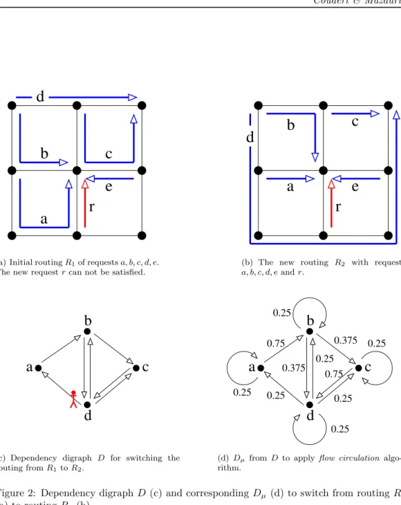
In WDM networks without wavelength conversion, the acceptation of a new connection request is subject to the availability of a lightpath (and so resources) from end to end in the network. Whatever the routing algorithm chosen, successive addition and removal of connections may lead to a poor usage of resources. Thus new connection requests might be rejected although the network has enough resources to handle the traffic pattern, up to the rerouting of some requests. For example, in Fig. 2(a), the network is a 9 nodes grid with one wavelength and 5 requests a, b, c, d, e. A new connection request r will be rejected in Fig. 2(a) although the routing of Fig. 2(b) is possible. Therefore, it is necessary to change from time to time the routing of established connections to improve the usage of resources, and so accept more traffic.

In this paper we concentrate on the reconfiguration phase, that is the problem of switch-ing the set of connections from current routswitch-ing, R1, to a new pre-computed routing, R2.

To solve this problem, several strategies are possible. For example, one may interrupt all connections requests that have to be rerouted and after restart them with their new routes in R2. This strategy is very simple, but requires to store a huge amount of traffic during

the reconfiguration phase and so requires large and costly buffers.

Another strategy is to reroute connection requests one after the other, as soon as des-tination resources (lightpath in the new routing) are available, minimizing the number of simultaneous interrupted requests during the reconfiguration. It corresponds to compute the process number (Sec. 2) in the dependency digraph [6]. This requires to compute the scheduling of the rerouting, taking into account that destination resources might be currently used by other connections. More precisely, resources assigned to request r in R2 might be

used by some request r0 in R1, thus request r0 has to be rerouted before r. We represent

these constraints by a digraph D = (V, A), the dependency digraph [6], in which each node corresponds to a request, and there is an arc from vertex u to vertex v if v must be rerouted before u.

For example to switch from routing R1 of Fig. 2(a) to routing R2 of Fig. 2(b), we

construct the dependency digraph D of Fig. 2(c). It has one node per connection that has to be rerouted, and so, connection e is not represented in D since it is not affected. It has an arc from a to b since connection b has to be switched before connection a. Similarly, it has arcs from b to c and from b to d since c and d must be switched before b, and so on.

When the digraph D is a dag (direct acyclic graph), the scheduling is straightforward, but in general, it may contain cycles. To break them, some requests have to be temporarily

4 Coudert & Mazauric

interrupted, thus removing some incident arcs in D. So, the optimization problem is to find a scheduling minimizing the number of requests simultaneously interrupted.

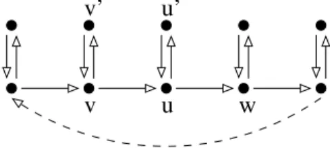
This problem has first been considered in [6]. They have proposed a heuristic algorithm based on the minimum feedback vertex set (mfvs) of D (i.e. the smallest subset S of nodes of D such that D − S is a dag) that performs well on small instances. This problem has also been considered in [3, 4] with a modeling in terms of cops-and-robber game [8]: the process number, denoted pn. It allows to use more advance theoretical concepts and so to design more efficient heuristic algorithms. For example, the digraph of Fig. 1 is such that |mfvs(D)| = n/2 and pn(D) = 2. So it is possible to reroute corresponding requests with only two requests simultaneously interrupted.

This paper starts in Sec. 2 with the modeling of our reconfiguration problem as a cops-and-robber game in the dependencies digraph, and so the definition of the process number. Then, in Sec. 3 we present some previous results linking pathwidth, vertex separation and process number. We also recall the heuristic algorithm proposed in [6]. In Sec. 4, we propose a heuristic algorithm to compute the process number of digraphs (i.e. maximum number of simultaneously interrupted requests) and the corresponding network reconfigura-tion strategy. Finally, in Sec. 5 we present simulareconfigura-tions results and analyze the efficiency of our heuristic algorithm compared to others.

2

Modeling

It has been proved in [3, 4] that the routing reconfiguration problem can be expressed as a cops-and-robber game [8], as for the pathwidth [10]. An interruption is represented by placing an agent on the corresponding node in D. A node is said processed when the corresponding request has been rerouted. If the node was occupied by an agent, then it can be reused. We call a process strategy a series of the three following actions (rules) allowing to reroute all requests with respect to the constraints represented by the digraph.

R1. Put an agent on a node (interrupt a connection).

R2. Remove an agent from a node if all its out-neighbors are either processed or occupied

by an agent (restart a connection on its final route when destination resources are available). The node is now processed (connection has been rerouted ).

R3. Process a node if all its out-neighbors are either processed or occupied by an agent1

(connection has been rerouted because destination resources are available).

A p-process strategy is a strategy which process the digraph using p agents and the process number, pn(D), is the smallest p such that a p-process strategy exists.

Clearly, pn(D) is upper bounded by the minimum feedback vertex set (mfvs) of D, that is the smallest subset S of nodes of D such that D − S is a dag. However, this bound is very

1_{In terms of cops and robber games in undirected graphs, rule R}

3expresses that the fugitive is forced to

move at each step.

Network Reconfiguration using Cops-and-Robber Games 5

large. For example, the digraph represented in Fig. 1 is such that |mfvs(D)| = n/2, but it can be 2-processed. For that, we put an agent on node u (rule R1). Then we apply rule R3

to process node u0. After, we put a second agent on node v (rule R1), process node v0 (rule

R3) and then process node v (rule R2). We repeat on the predecessor of v until processing

of the out-neighbor w of u. Finally, we apply rule R2 on u.

v

v’

u’

w

u

Figure 1: Digraph D such that pn(D) = 2 and mfvs(D) = n/2.

Notice also that when D is a dag the scheduling is straightforward using rule R3 from

the leaves (nodes with out-degree 0), and we have pn(D) = 0.

3

Previous work

First of all, it has been proved in [4] that vs(D) ≤ pn(D) ≤ vs(D) + 1, where vs(D) is the vertex separation of D. This implies that determining pn(D) is NP-complete in general, since it is also the case for vs(D). Furthermore, when D is a symmetric digraph, the same result holds for the underlying graph G. We also have vs(G) = pw(G), where pw(G) is the pathwidth of G [7, 10], and determining the pathwidth is NP-complete in general, approximable within O(log2|V (G)|), and there is no polynomial-time algorithm with an absolute error guarantee of |V (G)|1−ε _{for any ε > 0 [8, 2]. The same holds for the process}

number and so for the routing reconfiguration problem considered in [6, 4] and in this paper, thus motivating the development of an efficient heuristic algorithm.

Notice that for specific topologies it is possible to determine the process number in polynomial time. In particular, a characterization of digraphs with process number 1 and 2 is given in [4] as well as O(n+m) and O(n2(n+m)) respectively time complexity recognition algorithms.

When the digraph is composed of several strongly connected components (sccs), it is possible to process each scc independently, and then obtain the processing of D. For that, let {scci} be the set of sccs of D. Let also Dscc be the dag of sccs of D, thus containing

one node per component of {scci} and one arc from node i to node j iff D contains an arc

from some node u ∈ scci to some node v ∈ sccj. Then the processing of D consists in

processing the sccs sequentially following the order given by Dscc. Since sccs are processed

independently from each other the Lemma 1 follows. Notice that the computation of {scci}

and D_scc takes time O(n + m) using standard algorithms.

6 Coudert & Mazauric

c

b

r

e

d

a

(a) Initial routing R1of requests a, b, c, d, e.

The new request r can not be satisfied.

b

a

c

e

r

d

(b) The new routing R2 with requests

a, b, c, d, e and r.

d

b

c

a

(c) Dependency digraph D for switching the routing from R1to R2. 0.75

b

c

a

d

(d) Dµ from D to apply flow circulation

algo-rithm.

Figure 2: Dependency digraph D (c) and corresponding Dµ (d) to switch from routing R1

(a) to routing R2 (b).

Network Reconfiguration using Cops-and-Robber Games 7

Lemma 1. Given a digraph D and the set {scci} of its strongly connected components, we

have pn(D) = maxi{pn(scci)}.

We now recall the principle of the heuristic algorithm proposed in [6], HeurJS, to obtain the rerouting ordering of a digraph D = (V, A). It uses Lemma 1, and so we may assume that D is strongly connected. The main idea of HeurJS is to break elementary cycles. For that, it first computes the c elementary cycles of D using Johnson’s algorithm [5] and assigns to each node u the number α(u) of cycles it belongs to. Then it places an agent on the node u1

of maximum weight, thus breaking α(u1) cycles, updates the values of each remaining nodes

and repeats if α(ui) > 0, where uiis the new node of maximum weight. Let L be the set of

nodes covered by an agent. When all cycles have been broken, the digraph D − L is a dag and so can be 0-processed. Thus it processes D − L in appropriate order and then the nodes of L. The number of agents simultaneously used is |L|, and the time complexity of HeurJS is dominated by the computation of elementary cycles which takes time O((n + m)(c + 1)) [6]. Notice that this algorithm is exponential with the number c of elementary cycles, and so with the number n of nodes. Thus, HeurJS can only permit to solve the problem for small digraphs, as it has been designed for.

To the best of our understanding, HeurJS is in fact a heuristic algorithm for mfvs applied on each scc of D, following Lemma 1. Although shown to be quite efficient in practice through a large number of experimentations [6], its result could be far from optimality (see the example of Fig. 1).

4

Process strategy based heuristic algorithm

We now propose a heuristic algorithm HeurCM for solving the reconfiguration problem, taking advantages of the modeling with the process number proposed in [4]. This heuristic algorithm has polynomial time complexity, and with high probability improves upon HeurJS on the number of agents needed simultaneously (corresponding to the number of requests disturbed at the same time) in resulting strategy.

4.1

Flow circulation algorithm

Our algorithm is based on a flow circulation algorithm which has the objective of choosing the best candidate node to receive an agent and so to break a large set of cycles.

The principle is the following. Given a dependency digraph D = (V, A), each node u ∈ V is initially assigned a weight q0(u) = 1/ |V |. Then, at each round t, each node u

sends (1 − µ)qt(u)/d+(u) to each of its out-neighbors, where d+(u) = |Γ+(u)| with Γ+(u)

the set of out-neighbors of u in D, and µ ∈ (0, 1). Furthermore u keeps µqt(u) in order

to satisfy discrete Markov chain conditions. Indeed we transform the digraph D = (V, A) into Dµ = (Vµ, Aµ), such that Vµ = V and Aµ = A ∪ {(u, u), ∀u ∈ V }. In other words, we

add loops to each node of D. Clearly, the value of µ will influence the convergence time (i.e. number of rounds) of the flow circulation algorithm without significant impact on the

8 Coudert & Mazauric

final weights. Thus, we choose it close to 0, and so we will only slightly slow down the convergence time. We have for all u ∈ Dµ:

qt+1(u) = µqt(u) +

X

v∈Γ−_(u)

(1 − µ)qt(v)/d+(v) (1)

where Γ−_{(u) is the set of predecessors of u.}

After k rounds (the value of k will be discussed in Lemma 3), the node with maximum weight is the best candidate. With flow circulation algorithm, we expect that the node with maximum weight belongs to many cycles. So its removal from the digraph may break many cycles.

We will now evaluate the number k of rounds needed in the flow circulation algorithm. For that, we will first prove in Lemma 2 the convergence of the algorithm using a discrete Markov chain for which we define the set of states {u1, u2, ..., u|Vµ|} corresponding to the

nodes in Vµ and the transition matrix M associated to Dµ. We have for all x, y ∈ Vµ

M [x, y] =    (1 − µ)/d+_{(x) when y ∈ Γ}+_(x) µ when x = y 0 otherwise (2)

where Γ+(x) is the set of out-neighbors of x and d+(x) = |Γ+(x)|. We also define the vector of probability qt(Vµ) = (qt(u1), qt(u2), ..., qt(u|Vµ|)). qt(ui) (1 ≤ i ≤ |Vµ|) is the probability

that the state of the system is ui at step t ≥ 0.

Lemma 2. Let Dµ be a strongly connected digraph with loops. Whatever q0(Vµ), we have

limt→+∞qt(Vµ) = q(Vµ), where q(Vµ) is the unique stationary weights vector.

Proof. The proof relies on the discrete time Markov chain described previously, where the vector qt(Vµ) represents the probability of each state at step t ≥ 0 and M , associated to Dµ,

represents the transition matrix (see Equation 2).

From the Markov chains theory, we know that if the chain is irreducible and aperiodic (ergodic), then there exists a unique stationary distribution q(Vµ) whatever the initial state

q0(Vµ) [9].

• The irreducibility of the Markov chain is obvious because Dµ is a strongly connected

digraph. Indeed from each state x, there exists a positive probability to move to state y since there exists a path from x to y in Dµ.

• The Markov chain is aperiodic since Dµ is a strongly connected digraph with loops [9].

Fig. 2(c) consists on a digraph D = (V, A) of 4 nodes a, b, c, d. We construct Dµ =

(Vµ, Aµ) (Fig. 2(d)), adding loops in order to satisfy the Markov conditions described

before, even if it is not necessary in this example. The probabilities on the edges in Fig. 2(d) represent the Markov transition matrix (see Equation 2). We have qt(Vµ) =

(qt(a), qt(b), qt(c), qt(d)) such that q0(Vµ) = (0.25, 0.25, 0.25, 0.25). After 4 steps, we have

Network Reconfiguration using Cops-and-Robber Games 9

q4(Vµ) ≈ (0.1257, 0.2473, 0.2503, 0.3767), that is to say almost the stable vector q(Vµ) =

(0.125, 0.25, 0.25, 0.375). Thus node d has maximum weight.

The Markov chain admits always a stable state due to the artificial loop transition on each node. We now have to choose k sufficiently large to get the stable vector q(Vµ) with an

allowed error ε, that is εk≤ ε, where εk = ||qk(Vµ) − q(Vµ)||∞= O(|λ2|k), denoting λ2the

second largest eigenvalue of the transition matrix M . Thus we will obtain the node with the maximum weight.

Lemma 3. If |λ2| < ε1/k, then flow circulation algorithm computes q(Vµ) with an allowed

error ε.

Proof. From Perron-Frobenius Theorem [1], we know that the convergence time from qt(Vµ)

to the stationary vector q(Vµ) depends only of the second largest eigenvalue λ2 of M (the

first largest is always 1). Thus when |λ2|k < ε, the stable state is obtained with ||qk(Vµ) −

q(Vµ)||∞≤ ε.

Since computing the second largest eigenvalue value λ2of M is time consuming, in our

experiments we choose to fix arbitrarily k = n. For the example of Fig. 2(d), we thus have ||q4(Vµ) − q(Vµ)||∞≤ 0.003. Another example is with n = 500 requests and an allowed error

of ε = 0.01. Then, the flow circulation algorithm computes the stationary vector of the Markov chain if |λ2| < 0.99 (remember that the second largest eigenvalue is strictly lower

than 1, and that 0.99500< 0.01). Thus with a very high probability, we get the right stable vector and so a good candidate node for breaking cycles. See Sec. 5.1 for more details.

4.2

Heuristic algorithm

We assume that we are given a strongly connected digraph D. Otherwise, we apply our algorithm on each sccs, according to Lemma 1. We also assume that D is different than a single node digraph (otherwise we can process it easily) and it has been transformed into Dµ, but we say D for simplicity.

The heuristic algorithm, HeurCM, is described in Algorithm 1. It consists in choosing a node to place an agent using the flow circulation algorithm, and then it decomposes the digraph into sccs and repeats on each scci. Algorithm HeurCM maintains the set of nodes

covered by an agent, S, sorted by insertion dates. Also S.last is the latest inserted node that has not yet been processed. After any step of HeurCM, S may change: insertion of a new node covered by an agent (rule R1), and removal of nodes that can be processed (rule

R2). The number of agents used by HeurCM is thus the maximum size reached by S during

the algorithm, S. max.

The dependency digraph D of Fig. 2(c) is strongly connected and we apply HeurCM on it. We first apply flow circulation algorithm to choose the node to be covered by an agent, i.e. the node with maximum weight. So we choose d and add it to S (Fig. 2(c)). Since D − {d} is a dag, we can now process all remaining nodes (line 1) and finally process d. Thus HeurCM uses 1 agent in this example.

10 Coudert & Mazauric

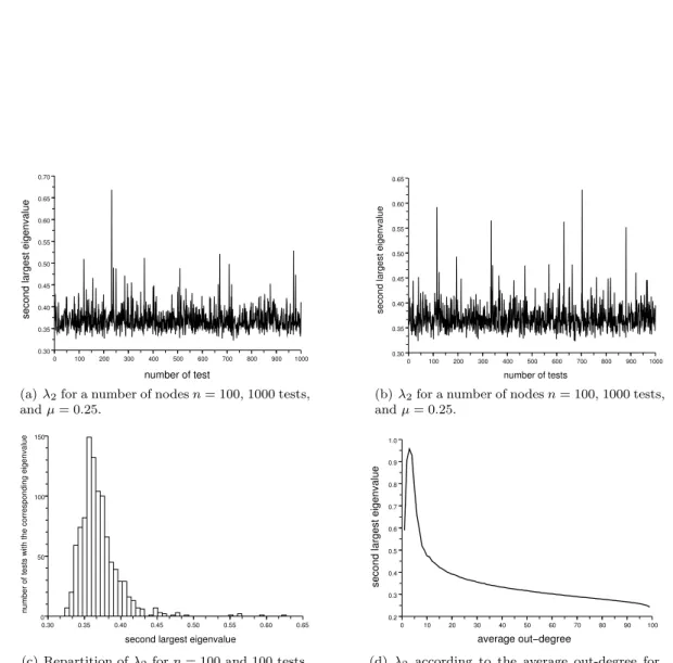
second largest eigenvalue

0 100 200 300 400 500 600 700 800 900 1000 0.30 0.35 0.40 0.45 0.50 0.55 0.60 0.65 0.70 number of test

(a) λ2for a number of nodes n = 100, 1000 tests,

and µ = 0.25. number of tests 0 100 200 300 400 500 600 700 800 900 1000 0.30 0.35 0.40 0.45 0.50 0.55 0.60 0.65

second largest eigenvalue

(b) λ2for a number of nodes n = 100, 1000 tests,

and µ = 0.25. 100 0.30 0.35 0.40 0.45 0.50 0.55 0.60 0.65 0 50 150

number of tests with the corresponding eigenvalue

second largest eigenvalue

(c) Repartition of λ2 for n = 100 and 100 tests.

average out−degree 0 10 20 30 40 50 60 70 80 90 100 0.2 0.3 0.4 0.5 0.6 0.7 0.8 0.9 1.0

second largest eigenvalue

(d) λ2 according to the average out-degree for

graphs with n = 100 nodes and µ = 0.25. 100 tests for each average out-degree.

Figure 3: Simulations: second largest eigenvalue.

Network Reconfiguration using Cops-and-Robber Games 11

number of agents required

0 100 200 300 400 500 600 700 800 900 1000 2.0 2.5 3.0 3.5 4.0 4.5 5.0 5.5 number of nodes

(a) Number of agents required by HeurCM to pro-cess digraphs of propro-cess number 2. 100 tests for each number of nodes 10k, k = 1..100.

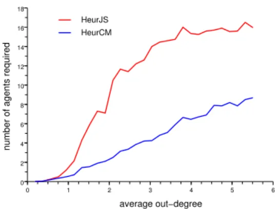
average out−degree 0 1 2 3 4 5 6 0 2 4 6 8 10 12 14 16 18 HeurJS HeurCM

number of agents required

(b) Number of agents required to process a 20 nodes random graph function of the average out-degree.

square root of the number of nodes

0 5 10 15 20 0 5 10 15 20 25 30 35 40 45 HeurCM Exact value

number of agents required

HeurJS

(c) Number of agents required to process n × n grids. time needed 0 2 4 6 8 10 12 0 50 100 150

square root of the number of nodes

(d) Computation time to process n × n grids.

Figure 4: Simulations: efficiency of HeurCM.

12 Coudert & Mazauric

Algorithm 1 HeurCM

Require: A strongly connected digraph D, the set of nodes covered by an agent S and the set of active nodes A

Ensure: The number of agents needed

1: Apply flow circulation on D.

2: Let u be one of the nodes of maximum weight. In case of equality we choose the closest node to S.last.

3: Place an agent on u: add it to S and remove it from A.

4: Process all the nodes whose can be processed updating S and A.

5: _{Decompose D ∩ {A} into sccs: {scc}i} 6: _{if {scc}i} is not empty then

7: HeurCM(scci, S), i = 1.. |{scci}| 8: end if

With the dependency digraph of Fig. 1, and w.l.o.g., node u is chosen among the set of nodes of maximum weights (all belonging to the main cycle) and added to S. Now, u0 is processed and then the digraph is decomposed into sccs, each being a 2-cycle, on which we apply recursively HeurCM (line 1). Thus, HeurCM will use only 2 agents.

When choosing the node of maximum weight at line 1 of Algorithm 1, it may happen that among the set of candidates, one of them allows to process a node of S. This is typically the case when the digraph is a bidirectional path u0, u1, u2, u3, . . . , ur, ur+1. W.l.o.g., we

may assume that u1 is chosen at line 1 and so added to S. We process node u0, and we

repeat the algorithm on u2, u3, . . . , ur+1. Now, candidates will be u3and ur(the symmetry

of the graph give same weights for u3and ur), but u3is clearly a better choice since is allows

to process u2and after u1 thus releasing one agent. It is why in case of equality, we choose

the closest node to S.last.

Lemma 4. The worst case time complexity of HeurCM is O(kn(n + m)).

Proof. Each flow circulation round takes time O(k(n + m)) and in the worst case D ∩ {A} = D − {u} is a single scc.

Finally, note that the rerouting strategy follows directly our algorithm. With HeurCM, it is sufficient to know entering and leaving dates in S and in A to know when a connection is suspended (enter in S) or switched to its new route (leave S or A).

5

Simulations

In this section, we first analyze further the convergence time of the flow circulation algorithm. Then, we analyze the performance of our heuristic algorithm HeurCM.

Network Reconfiguration using Cops-and-Robber Games 13

5.1

Convergence time of flow circulation

We present here some simulations showing that the second eigenvalue λ2 of M respects

almost surely the conditions given in Lemma 3. For that, we have designed different kinds of random Markov matrices Mn×n.

• A fully random matrix, that is to say for each line of M (i.e. for each node), the out-degree and the out-neighbors are chosen randomly and uniformly. Fig. 3(d) and Fig. 3(b) show the distribution of λ2 for n = 100 and 1000 tests. For these two simulations, λ2 is

always lower than 0.7. Furthermore, Fig. 3(c) describes that with high probability, λ2 is

small.

• We have designed a random matrix with constant average out-degree d, that is to say for each line of M , d is a binomial distribution of parameters d/n and n. Then the out-neighbors are chosen randomly and uniformly. Fig. 3(d) shows the value λ2 for each

possible average degree for a digraph of 100 nodes. Note that for each average out-degree, 100 tests has been done. λ2 is very small (lower than 0.5) except for very small

average out-degree.

5.2

Simulations of HeurJS and HeurCM

We have implemented and analysed the efficiency of HeurJS and our algorithm HeurCM (in term of number of agents simultaneously required and in term of computation time).

• In [4], a characterization of the graphs with process number 2 is done and Fig. 4(a) shows the approximate process number computed by HeurCM for these graphs. The number of agents increases very slowly with the number of nodes (requests). For a digraph of 1000 nodes, the number of agents required is almost 5.

• For a symmetric grid Gn×n, Fig. 4(c) shows that the approximate process number

computed by HeurCM is closed to the exact value (n + 1 if n > 2) whereas the number of agents required by HeurJS increases exponentially. Furthermore, the computation time is very smaller for HeurCM compared to HeurJS (Fig. 4(d)), because a grid is a strongly connected symmetric digraph and there is an exponential number of cycles.

• For a 20 nodes random graph, starting with an average out-degree d closed to 0, increasing it until d = 6, Fig. 4(b) shows that HeurCM requires less agents that HeurJS.

6

Conclusion

In this paper, we have proposed a new heuristic algorithm for the reconfiguration problem of switching the connections from one routing to another with objective of minimizing the number of connections simultaneously interrupted. This new heuristic algorithm is based on a modeling with cops-and-robbers games and improves upon previous proposal in both efficiency and computation time, as shown by our simulation results.

The next step is to design an exact and efficient exponential algorithm viable in practice for digraphs with a small number of nodes.

14 Coudert & Mazauric

Acknowledgments

This work has been partially supported by ANR JC OSERA, r´egion PACA, European projects IST FET AEOLUS and COST 293 Graal.

References

[1] O. Axelsson. Iterative solution methods. Cambridge University Press, 1994.

[2] H.L. Bodlaender, J.R. Gilbert, H. Hafsteinsson, and T. Kloks. Approximating treewidth, pathwidth, frontsize, and shortest elimination tree. Journal of Algorithms, 18(2):238–255, March 1995.

[3] D. Coudert, S. Perennes, Q.-C. Pham, and J.-S. Sereni. Rerouting requests in wdm networks. In AlgoTel’05, pages 17–20, Presqu’ˆıle de Giens, France, mai 2005.

[4] D. Coudert and J-S. Sereni. Characterization of graphs and digraphs with small process number. Research Report 6285, INRIA, September 2007.

[5] Donald B. Johnson. Finding all the elementary circuits of a directed graph. SIAM Journal on Computing, 4(1):77–84, 1975.

[6] N. Jose and A.K. Somani. Connection rerouting/network reconfiguration. Design of Reliable Communication Networks (DRCN), pages 23–30, October 2003.

[7] N. G. Kinnersley. The vertex separation number of a graph equals its pathwidth. Information Processing Letters, 42(6):345–350, 1992.

[8] M. Kirousis and C.H. Papadimitriou. Searching and pebbling. Theoretical Computer Science, 47(2):205–218, 1986.

[9] S.P. Meyn and R.L. Tweedie. Markov Chains and Stochastic Stability. Springer-Verlag, London, 1993.

[10] N. Robertson and P. D. Seymour. Graph minors. I. Excluding a forest. J. Combin. Theory Ser. B, 35(1):39–61, 1983.

Unité de recherche INRIA Sophia Antipolis

2004, route des Lucioles - BP 93 - 06902 Sophia Antipolis Cedex (France)

Unité de recherche INRIA Futurs : Parc Club Orsay Université - ZAC des Vignes 4, rue Jacques Monod - 91893 ORSAY Cedex (France)

Unité de recherche INRIA Lorraine : LORIA, Technopôle de Nancy-Brabois - Campus scientifique 615, rue du Jardin Botanique - BP 101 - 54602 Villers-lès-Nancy Cedex (France)

Unité de recherche INRIA Rennes : IRISA, Campus universitaire de Beaulieu - 35042 Rennes Cedex (France) Unité de recherche INRIA Rhône-Alpes : 655, avenue de l’Europe - 38334 Montbonnot Saint-Ismier (France) Unité de recherche INRIA Rocquencourt : Domaine de Voluceau - Rocquencourt - BP 105 - 78153 Le Chesnay Cedex (France)

Éditeur

INRIA - Domaine de Voluceau - Rocquencourt, BP 105 - 78153 Le Chesnay Cedex (France)

http://www.inria.fr ISSN 0249-6399