HAL Id: hal-02103943
https://hal.archives-ouvertes.fr/hal-02103943
Submitted on 19 Apr 2019
HAL is a multi-disciplinary open access
archive for the deposit and dissemination of
sci-entific research documents, whether they are
pub-lished or not. The documents may come from
teaching and research institutions in France or
abroad, or from public or private research centers.
L’archive ouverte pluridisciplinaire HAL, est
destinée au dépôt et à la diffusion de documents
scientifiques de niveau recherche, publiés ou non,
émanant des établissements d’enseignement et de
recherche français ou étrangers, des laboratoires
publics ou privés.
Functional Programs (Technical Report)
Martin Avanzini, Ugo Dal Lago, Alexis Ghyselen
To cite this version:
Martin Avanzini, Ugo Dal Lago, Alexis Ghyselen. Type-Based Complexity Analysis of Probabilistic
Functional Programs (Technical Report). [Research Report] INRIA Sophia Antipolis; University of
Bologna; ENS Lyon. 2019. �hal-02103943�
of Probabilistic Functional Programs (Technical Report)
MARTIN AVANZINI,
INRIA Sophia AntipolisUGO DAL LAGO,
University of Bologna, INRIA Sophia AntipolisALEXIS GHYSELEN,
ENS LyonWe show that complexity analysis of probabilistic higher-order functional programs can be carried out
compositionally by way of a type system. The introduced type system is a significant extension of linear
dependent types. On the one hand, the presence of probabilistic effects requires adopting a form ofdynamic
distribution type, subject to a coupling-based subtyping discipline. On the other hand, recursive definitions are
proved terminating by way of ranking functions. We prove not only that the obtained system, calleddℓRPCF,
provides a sound methodology for average case complexity analysis, but is alsoextensionally complete, in the
sense that all average case polytime Turing machines can be encoded as a term typable indℓRPCF.
1 A PROBABILISTIC FUNCTIONAL LANGUAGE EXTENDING AFFINE PCF
In this section we introduce the programming languagedℓRPCF that we consider throughout this work. It is basically an affine version of Plotkin’s, extended with an operatorUnif for sampling from uniform, discrete distributions. The type system we introduce in this section does not guarantee any complexity propriety.
Statics: The sets of terms, values and types are generated by the following grammars: Terms t,u ::= v
|
v w|
let x = t in u|
match v with { z 7→ t | s 7→ w }|
let ⟨x,y⟩ = v in tValues v, w ::= x
|
z|
s(v)|
Unif|
λx.t|
fix x.v|
⟨v, w⟩ Types T ,U ::= Nat|
T ⊸ U|
T ⊗ UTerms are restricted toA-normal forms. In this setting, the application t u is recovered by let x = t in let y = u in x y. Apart from our sampling operator Unif, the constructors are standard. We follow the usual convention where applicationt u binds to the left, whereas λ-abstraction λ.t binds to the right. Terms which are not values are calledactive. For an integern ∈ N, we denote with n the values(. . . , s(z), . . . ), with n occurrences of s. The capture free substitution of variable x by valuev in t is denoted t[x := v].
We impose a linear typing regime on terms. The typing rules are presented in Figure 1. The statementΓ | Θ ⊢ t : T means that under the (linear) typing context Γ and the global typing context Θ the term t receives the type T . Here, a typing context Γ is a non-ordered sequence of the form x1:T1. . . xn :Tn. The union of two linear type contextsΓ and ∆, denoted Γ, ∆, is defined only if for each variablex with (x : T ) ∈ Γ and (x : U ) ∈ ∆, it holds that T = U = Nat. Global type contexts Θ, used to treat recursive functions, are either empty or consist of a unique hypothesisx : T ⊸ U . In rule Fix,ℓΓ denotes a typing context where all variables are given the type Nat. For closed terms t, we abbreviate∅ | ∅ ⊢ t : T by ⊢ t : T . We remark that this affine type system permits duplication of values of base type, whereas duplication of values of functional types is prohibited.
Authors’ addresses: Martin Avanzini, INRIA Sophia Antipolis; Ugo Dal Lago, University of Bologna, INRIA Sophia Antipolis; Alexis Ghyselen, ENS Lyon.
2019. XXXX-XXXX/2019/1-ART $15.00 https://doi.org/10.1145/nnnnnnn.nnnnnnn
(x : T ) ∈ Γ or (x : T ) ∈ Θ
Γ | Θ ⊢ x : T (Ax) Γ | Θ ⊢ z : Nat(Zero)
Γ | Θ ⊢ v : Nat
Γ | Θ ⊢ s(v) : Nat(Succ)
Γ | Θ ⊢ Unif : Nat ⊸ Nat(Unif)
Γ | Θ ⊢ v : T ⊸ U ∆ | Θ ⊢ w : T Γ, ∆ | Θ ⊢ v w : U (App) Γ, x : T | Θ ⊢ t : U Γ | Θ ⊢ λx.t : T ⊸ U(Abs) ℓΓ | (x : T ⊸ U ) ⊢ v : T ⊸ U Γ, ℓΓ | Θ ⊢ fix x.v : T ⊸ U (Fix) Γ | Θ ⊢ t : T ∆, x : T | Θ ⊢ u : U Γ, ∆ | Θ ⊢ let x = t in u : U (Let) Γ | Θ ⊢ v : T ∆ | Θ ⊢ w : U Γ, ∆ | Θ ⊢ ⟨v, w⟩ : T ⊗ U (⊗i) Γ | Θ ⊢ v : T ⊗ T′ ∆, x : T ,y : T′|Θ ⊢ t : U Γ, ∆ | Θ ⊢ let ⟨x,y⟩ = v in t : U (⊗e) Γ | Θ ⊢ v : Nat ∆ | Θ ⊢ t : T ∆ | Θ ⊢ w : Nat ⊸ T
Γ, ∆ | Θ ⊢ match v with { z 7→ t | s 7→ w } : T (Match)
Fig. 1. Affine type system for probabilistic PCF
Dynamics: Following [Dal Lago and Grellois 2017], we can givedℓRPCF an operational semantics in terms of a binary relation⇒ on distributions. On the non-probabilistic fragment of our language, i.e., on terms without any occurrences ofUnif, the semantics can be seen isomorphic to the usual (weak) call-by-value reduction relation.
A(discrete) valuation on a countable setX is a function v : X → [0, +∞]. The support of v is given bySupp(v) ≜ {x ∈ X | v(x) > 0}. It is called finite if its support is finite. The set of valuations onX is denoted V (X ). We may denote a valuation v also by {v(x) : x}x ∈Supp(v) or {v(x1) :x1, . . . ,v(xn) :xn} whenSupp(v) = {x1, . . . , xn} is finite. Scalar multiplicationp · v and finite sumÍi ∈Iviare defined point-wise. A(discrete) distribution onX is a valuation D : X → [0, 1] such thatÍ D ≜ Íx ∈XD(x) ≤ 1. It is called proper if Í D = 1. The set of distributions is closed under scalar multiplication, but not necessarily under finite sum. We define the relation≤ on distributions such thatD ≤ E if D(x) ≤ E(x) for all x ∈ X . For a distribution D on terms, Da+a/vDvindicates the decomposition ofD, i.e. D = Da+ Dv, so that the supports ofDaand Dv consist of active terms and values, respectively.
The reduction relation⇒ is itself based on an auxiliary relation →, depicted in Figure 2, which maps active terms to distributions. Ift → {p1:t1, . . . , pn :tn}, thentishould be understood as a one-step reduct oft with probability pi. All rules but the one definingUnif follow the standard operational semantics ofPCF. A termUnif n reduces to the uniform distribution on (0,n) wrt. →. Based on the auxiliary relation→, the relation ⇒ is given by the following inference rule.
D= {pi :ti |i ∈ I} +a/vDv ∀i ∈ I, ti → Ei D ⇒ Dv+ Íi ∈Ipi· Ei
The type system is coherent with the reduction rules, in particular, the type system enjoys subject reduction and progress in the following sense.
Proposition 1.1 (Subject Reduction and Progress). Lett be such that ⊢ t : T holds. (1)Ift → {pi :ti |i ∈ I} (with pi > 0 for all i) then for all i ∈ I, we have ⊢ ti :T . (2)The termt is in normal form for → if and only if t is a value.
(λx.t) v → {1 : t[x := v]} (fix x.w) v → {1 : w[x := fix x.w] v}
Unif n → { 1
n+1:m | 0 ≤ m ≤ n}
match z with { z 7→ t | s 7→ w } → {1 : t} match s(v) with { z 7→ t | s 7→ w } → {1 : w v}
let x = v in t → {1 : t[x := v]} let ⟨x,y⟩ = ⟨v,w⟩ in t → {1 : t[x := v][y := w]}
t → {pi :ti |i ∈ I}
let x = t in u → {pi :let x = tiin u | i ∈ I}
Fig. 2. Reductions rules on distributions
Subject reduction, i.e. Property 1.1.1, implies in particular that distributions of well typed terms are closed under⇒ reductions.
We denote with⇒∗the reflexive and transitive closure of⇒, and we denote with ⇒nthenth iteration of the reduction relation⇒. We remark that the set of finite distributions is closed under ⇒. Finally, let D ⇒v EvifD ⇒ Ea+a/vEv, and similarly the relations⇒vnand⇒v∗ are defined in terms of⇒nand⇒∗, respectively. Note that ifD ⇒nvEnwheren ∈ N, then Em ≤ Enwhenever m ≤ n. Likewise, we define the relation ⇒a. Thesemantics of a term is a distribution on values defined as
Jt K =sup{D |t ⇒ ∗
v D}. This is a well-posed definition because distributions form an ωCPO.
Example 1.2 (Biased Random Walk). For two termst and u, let us denote by t ⊕nu the term let p = Unif n in (match p with { z 7→ t | s 7→ λq.u }) for fresh variables p and q. Then t ⊕nu reduces with probability 1
n+1tot, and with probability n
n+1tou. Consider the term rwalk ≜ fix rw.λn.match n with { z 7→ z | s 7→ λm.rw (s(s(m))) ⊕2rw m } . Its recursive calls gives a biased random walk, withrwalk n+ 1 reducing to rwalk n + 2 with probability 1
3, and with probability 2
3 torwalk n. For any n ∈ N, rwalk n reduces to z almost surely, and hence
Jrwalk nK = {1 :z}.
In this work, we are interested in average case complexity analysis, in terms of reduction steps. In a probabilistic setting, the reduction length from a termt can be understood as a random variable St on N ∪ {∞}, with P(S = n) being the probability that t evaluates to normal form in n steps, or diverges in the casen = ∞. The expected runtime of a term t is then defined in terms of its expectation E(St) ≜ ∞ Õ n=0 P(St > n) .
Here, P(St > n) gives the probability that a reduction takes strictly more than n steps. In our setting, this probability is expressed byÍ Dan, forDanthe distribution of active terms reachable inn steps from t, i.e., t ⇒na Dna. This motivates the following definition, compare [Avanzini et al. 2018] for further justification of this definition.
Definition 1.3 (Expected Runtime). The expected runtime of a termt is defined by E(t) ≜ Í∞
We remark that E(v) = 0 for any value v, and if t → {pi :ti |i ∈ I} then E(t) = 1+Íi ∈Ipi·E(ti). 2 THE TYPE SYSTEM
This section is devoted to introducing the main object of study of this paper,dℓRPCF, a monadic, linear dependent type system for reasoning about expected runtimes. This system borrows ideas from the dependent type systemdℓPCF introduced by Dal Lago and Petit [Dal Lago and Petit 2012] for reasoning about the runtime of deterministic programs and from the affine, monadic type system introduced by Dal Lago and Grellois [Dal Lago and Grellois 2017] for proving almost sure termination of probabilistic programs.
2.1 Indexes, Types and Subtyping
As in the case of linear dependent types, base types are annotated with refinement constraints. Constraints are formed overindex terms, i.e., first-order terms generated freely from a set of index symbols I and index variables V, denoted byf ,д, . . . and a,b, . . . respectively. Each symbol f ∈ I is associated with a natural numberar(f ), its arity.
Definition 2.1 (Indices). Natural indicesI, J, . . . and rational indices P, Q, . . . are generated from function symbolsI and index variables V according to the following grammar:
I, J ≜ a
|
f (I1, . . . , Iar(f ))|
Õa ≤I
J
|
maxa ≤IJ P, Q ≜ I J .We useA, B, . . . to denote natural and rational indices. We assume that each function symbol f ∈ I comes equipped with an interpretationJ f K : Nar(f )→ N. We do not put any constraints on these functions, apart from computability. Given a valuationρ : V → N, the interpretation of symbols is extended homomorphically to indices:JaKρ ≜ ρ(a) for index variables a,
J f (I1, . . . , In)Kρ ≜ J f K(JI1Kρ, . . . ,JInKρ) andJ
I JKρ ≜ JI Kρ J J Kρ ifJJ Kρ , 0. In the case JJ Kρ= 0, J I JKρis undefined. Note that for any valuationρ and index A,
JAKρis computable. We suppose thatI contains for each n ∈ N a constant n interpreted byJnK ≜ nas well as symbols+ and · interpreted as addition and multiplication, respectively. For an indexI over variables a1, . . . , ak andJ over a1, . . . , ak,b, we define a special symbolÍb ≤I J with an interpretation satisfying
J Í
b ≤IJKρ= Ín ≤JI KρJJ Kρ[b7→n] . Likewise, we define the maximum of a bounded sequence. We will often, by an abuse of notation, use operations on rational indexes. For example, I
J +I
′
J′ denotes the rational index
I ·J′+I′·J
J ·J′ . For
an indexA, we define the substitution of a in A by a natural index J, that we note A{J/a}, in the obvious way.
Definition 2.2 (Constraints on Indexes). Letϕ ⊆ V be a set of index variables. A constraint C onϕ is an expression of the form A R B where A, B are indexes with free variables in ϕ. Here, R denotes a relation between integers or rationals. Usually, we use relations in the set{≤, <, =, ,} but we could use any computable relation. Finite sets of constraints are denoted byΦ. We say that an index valuationρ : ϕ → N satisfies a constraint A R B, in notation ρ ⊨ A R B, ifJAKρandJBKρ are defined and
JAKρRJBKρ holds. Likewise,ρ ⊨ Φ if ρ ⊨ A R B holds for all (A R B) ∈ Φ. In the same way, we say thatϕ; Φ ⊨ A R B when for any ρ : ϕ → N such that ρ ⊨ Φ then ρ ⊨ A R B.
Definition 2.3 (Linear Dependent Types). Linear dependent typesσ, τ and dynamic distribution types (DDTs)µ, ν are defined as follows:
linear dependent types σ, τ ≜ Nat(a | Φ)
|
σ ⊗ τ|
σ⊸ arrow types σ⊸≜ σ ⊸ µ|
∀a : Φ.σ⊸ dynamic distribution types µ, ν ≜ {P : σ | a ≤ I }A typeNat(a | Φ) represents the set of naturals n for which Φ{n/a} is true. It should thus be understood as an existential type bindinga, with a occurring free in Φ. For instance, Nat(a | a ≤ n) represents a natural number between zero andn ∈ N, and more generally, Nat(a | a ≤ J) would represent naturals bounded byJ. For brevity, we may abbreviate with Nat(I) the type Nat(a | a = I), specifically,Nat(b) denotes Nat(a | a= b).
Our type system admits polymorphism over indices in the form of bounded universal quantifica-tion over funcquantifica-tion types. The variablea in a type ∀a : Φ.σ⊸can be free inΦ and σ⊸, whereas it is bound in∀a : Φ.σ⊸. We will sometimes abbreviate an arrow typeσ⊸as∀a : Φ.σ ⊸ µ, with a being a list of index variables andΦ a list of sets of constraints.
Finally, the dynamic distribution type{P : σ | a ≤ I } can be understood as a monadic type for probabilistic computations which yield with probabilityP an element of type σ.
In the dynamic distribution type,a can be free in P and σ but not in I, and it will be considered bound in{P : σ | a ≤ I }. For instance, the DDT { 1
I +1 :Nat(b) | b ≤ I } represents a probabilistic computation that evaluates to a natural number uniformly distributed in the interval from 0 toI. This is indeed the type that our system will assign to the termUnif t, where t is of type Nat(I). We may abbreviate withσ the DDT {1 : σ | a ≤ 0} representing a dirac distribution, for a not occurring free inσ. Thereby, we may assign to terms of function type that exhibit no probabilistic behaviour the usual typeτ ⊸ σ, instead of τ ⊸ {1 : σ | a ≤ 0}.
Types in general are indicated byζ , ξ , . . . . We consider types equal modulo renaming of bound variables and denote byζ {I/a} the capture-avoiding substitution of the index variable a by I in the typeζ . All types are defined under some restrictions, such as the fact that the sum of probabilities in a distribution must be equal to 1. These restrictions are captured in our notion of valid type, see Figure 3. Notice that if an indexA is valid under ϕ; Φ, then for all valuations ρ : ϕ → N such that ρ ⊨ Φ,JAKρ is well defined. From now on, given a contextϕ; Φ, we will only consider valid types without always reminding it.
2.2 Subtyping
Since our type annotations give a form of refinement, it should always be possible to relax a refinement to a more liberal one. To this end, we introduce a subtyping relation on types. The core of our subtyping relation, presented in Figure 4 is fairly standard. A typeNat(a | Φ1) is a subtype of Nat(a | Φ2) ifΦ1impliesΦ2. One natural way to extend subtyping to DDTs is to lift the subtyping relation component-wise, i.e.{P : σ | a ≤ I } is a subtype of {P : τ | a ≤ I } if σ is a subtype of τ , for all a = 0, . . . , I. Although simple, this extension is too rigid to deal with more interesting functions. Instead, our treatment of subtyping for DDTs is based on the notion ofprobabilistic coupling, already studied in computer science [Barthe et al. 2017].
Intuitively, in the couplingS ◁⊑⟨{P : σ | a ≤ I }&{Q : τ | b ≤ J }⟩, S can be seen as a distribution over the set{(σ, τ ) | a ≤ I,b ≤ J, σ R τ } and S denotes the fraction of the probability P for σ that will contribute to the probabilityQ for τ . For example, if σ R τ and σ′Rτ , then {1
2 :σ, 1 2 :σ ′} and {1 4 :σ, 1 4 :σ ′,1
2 :τ } are coupled by the distribution { 1 4 :(σ, τ ), 1 4 :(σ ′, τ ),1 4 :(σ, σ), 1 4 :(σ ′, σ′)}. Subtyping is extended to function types in the standard way:σ ⊸ µ ⊑ τ ⊸ ν holds if µ ⊑ ν andσ ⊑ τ . Then for quantification, on the right we internalize quantification in the set of variables
Indices and constraints: FV(I ) ⊆ ϕ ϕ; Φ ⊢ I valid ϕ; Φ ⊢ I valid ϕ; Φ ⊢ J valid ϕ; Φ ⊨ J , 0 ϕ; Φ ⊢ IJvalid ϕ; Φ ⊢ A valid ϕ; Φ ⊢ B valid ϕ; Φ ⊢ A R B valid
ϕ; Φ ⊢ A R B valid for all (A R B) ∈ Φ′
ϕ; Φ ⊢ Φ′ valid Types: a < ϕ (ϕ, a); Φ ⊢ Φavalid ϕ; Φ ⊢ Nat(a | Φa) valid ϕ; Φ ⊢ σ valid ϕ; Φ ⊢ τ valid ϕ; Φ ⊢ σ ⊗ τ valid ϕ; Φ ⊢ σ valid ϕ; Φ ⊢ τ valid ϕ; Φ ⊢ σ ⊸ τ valid a < ϕ (ϕ, a); Φ ⊢ Φavalid (ϕ, a); (Φ, Φa) ⊢σ⊸valid (ϕ, a); (Φ, Φa) ⊨ a ≤ I for some index I
ϕ; Φ ⊢ ∀a : Φa.σ⊸valid
ϕ; Φ ⊢ I valid (ϕ, a); (Φ, a ≤ I) ⊢ P valid (ϕ, a); (Φ, a ≤ I) ⊢ σ valid ϕ; Φ ⊨ Ía ≤IP = 1
ϕ; Φ ⊢ {P : σ | a ≤ I } valid
Fig. 3. Validity of indices, constraints and types
and constraints, and on the left subtyping correspond to finding an instantiation for the quantified variable. Finally, we add the conversion rule. Informally, this rule describe that a function of type Nat(a | Φa) ⊸ µ could be given equivalently the type ∀a : Φa.Nat(a) ⊸ µ.
Example 2.4 (Subtyping for Arrow Types). We give a common example of subtyping for arrow types:⊢ (∀a : a ≤ I .Nat(a) ⊸ Nat(a)) ⊑ Nat(b | b ≤ I ) ⊸ Nat(c | c ≤ I ).
Nat(b | b ≤ I ) ▷ b : (b ≤ I ).Nat(b)
b; (b ≤ I) ⊨ b ≤ I b; (b ≤ I) ⊢ Nat(b) ⊸ Nat(b) ⊑ Nat(b) ⊸ Nat(c | c ≤ I) b; (b ≤ I) ⊢ (∀a : a ≤ I.Nat(a) ⊸ Nat(a)) ⊑ Nat(b) ⊸ Nat(c | c ≤ I)
⊢ (∀a : a ≤ I .Nat(a) ⊸ Nat(a)) ⊑ ∀b : (b ≤ I ).Nat(b) ⊸ Nat(c | c ≤ I )
⊢ (∀a : a ≤ I .Nat(a) ⊸ Nat(a)) ⊑ Nat(b | b ≤ I ) ⊸ Nat(c | c ≤ I )
And then we can conclude easily. The important point is the use of conversion rule. This conversion allows us to "extract" the elements ofNat(b | b ≤ I ) in order to use them in the instantiation for the∀ − L rule. Notice that without conversion, there is no instantiation J of a such that⊢ Nat(b | b ≤ I ) ⊑ Nat(J )
This definition of subtyping still verifies the conditions to be a preorder, as explained by the following lemma.
Lemma 2.5 (Subtyping and Preorder). Letϕ be an set of index variables and Φ be a set of constraints. Letζ , ζ′, ζ′′be valid types underϕ; Φ. Then ϕ; Φ ⊢ ζ ⊑ ζ and if ϕ; Φ ⊢ ζ ⊑ ζ′and ϕ; Φ ⊢ ζ′⊑ζ′′
thenϕ; Φ ⊢ ζ ⊑ ζ′′.
In order to work more conveniently with subtyping in the technical parts, we combine all conversion and rule for arrow types into one. This is described by the rules in Figure 5. We prove that this subtyping system and the previous one are equivalent. The only interesting cases are arrow types. First, we show how to simulate this alternative rule in the original type system. Notice that elements can be simulated by a chain of conversion rules and ∀ − R rules, as the only difference between conversion andelements is the fact that conversion deals with a tensor type one by one whereaselements does everything simultaneously.
Conversion: Nat(a | Φ) ▷ a : Φ.Nat(a) σ ▷ a : Φ.σ′ σ ⊗ τ ▷ a : Φ.(σ′⊗τ ) τ ▷ a : Φ.τ′ σ ⊗ τ ▷ a : Φ.(σ ⊗ τ′) Conversion Rule: σ ▷ a : Φa.σ′ a < ϕ ϕ; Φ ⊢ τ ⊑ ∀a : Φa.σ′⊸ µ ϕ; Φ ⊢ τ ⊑ σ ⊸ µ (Conv) Coupling
(ϕ, a,b); (Φ, a ≤ I,b ≤ J) ⊢ S valid (ϕ,b); (Φ,b ≤ J) ⊨ Ía ≤IS = Q
(ϕ,b); (Φ, a ≤ I) ⊨ Íb ≤JS = P (ϕ, a,b); (Φ, a ≤ I,b ≤ J, S , 0) ⊢ σ ⊑ τ ϕ; Φ ⊢ S ◁⊑⟨{P : σ | a ≤ I }&{Q : τ | b ≤ J }⟩ (Coupling) Structural Rules: (ϕ, a); (Φ, Φ1) ⊨ Φ2 ϕ; Φ ⊢ Nat(a | Φ1) ⊑ Nat(a | Φ2) (Nat) ϕ; Φ ⊢ τ ⊑ σ ϕ; Φ ⊢ µ ⊑ ν ϕ; Φ ⊢ σ ⊸ µ ⊑ τ ⊸ ν (⊸) ϕ; Φ ⊢ σ1⊑τ1 ϕ; Φ ⊢ σ2⊑τ2 ϕ; Φ ⊢ σ1⊗σ2⊑τ1⊗τ2 (⊗) ϕ; Φ ⊨ Φa{I/a} ϕ; Φ ⊢ σ {I/a} ⊑ τ ϕ; Φ ⊢ ∀a : Φa.σ ⊑ τ (∀-L) (ϕ, a); (Φ, Φa) ⊢σ ⊑ τ ϕ; Φ ⊢ σ ⊑ ∀a : ϕa.τ (∀-R) ∃S, ϕ; Φ ⊢ S ◁⊑⟨µ&ν⟩ ϕ; Φ ⊢ µ ⊑ ν (DDT)
Fig. 4. Subtyping Rules
elements(Nat(a | Φa))= a; Φa;Nat(a) elements(σ⊸)= ·; ·; σ⊸
elements(σ) = ϕ; Φ;τ elements(σ′)= ϕ′;Φ′;τ′ ϕ ∩ ϕ′= ∅
elements(σ ⊗ σ′)= (ϕ, ϕ′); (Φ, Φ′); (τ ⊗ τ′)
elements(τ ) = ϕτ;Φτ;τ′
I such that (ϕ,b, ϕτ); (Φ, Φb, Φτ) ⊨ Φa{I/a}
(ϕ,b, ϕτ); (Φ, Φb, Φτ) ⊢τ′⊑σ {I/a} (ϕ,b, ϕτ); (Φ, Φb, Φτ) ⊢µ{I/a} ⊑ ν
ϕ; Φ ⊢ ∀a : Φa.σ ⊸ µ ⊑ ∀b : Φb.τ ⊸ ν
Fig. 5. Alternative Subtyping Rules
elements(τ ) = ϕτ;Φτ;τ′ (ϕ,b, ϕτ); (Φ, Φb, Φτ) ⊢σ {I/a} ⊸ µ{I/a} ⊑ τ′⊸ ν (ϕ,b, ϕτ); (Φ, Φb, Φτ) ⊨ Φa{I/a} (ϕ,b, ϕτ); (Φ, Φb, Φτ) ⊢∀a : Φa.σ ⊸ µ ⊑ τ′⊸ ν (ϕ,b); (Φ, Φb) ⊢∀a : Φa.σ ⊸ µ ⊑ τ ⊸ ν ϕ; Φ ⊢ ∀a : Φa.σ ⊸ µ ⊑ ∀b : Φb.τ ⊸ ν
Now we need to prove the converse, ifϕ; Φ ⊢ σ⊸⊑τ⊸can be derived in the original subtype system, then it can be derived in the alternative one. We prove this by induction on the original subtype system.
•
τ ▷ b : Φb.τ′ b < ϕ ϕ; Φ ⊢ ∀a : Φa.σ ⊸ µ ⊑ ∀b : Φb.τ′⊸ ν
ϕ; Φ ⊢ ∀a : Φa.σ ⊸ µ ⊑ τ ⊸ ν
(Conv)
By induction hypothesis, we have :
elements(τ′)= (b′, ϕ τ); (b′= b, Φτ);τ′′ I such that (ϕ,b,b′ϕ τ); (Φ,b′= b, Φb, Φτ) ⊨ Φa{I/a} (ϕ,b,b′, ϕ τ); (Φ, Φb,b′= b, Φτ) ⊢τ′′⊑σ {I/a} (ϕ,b,b′, ϕ τ); (Φ, Φb,b′= b, Φτ) ⊢µ{I/a} ⊑ ν ϕ; Φ ⊢ ∀a : Φa.σ ⊸ µ ⊑ ∀b : Φb.τ′⊸ ν
The form ofelements(τ′) can be explained by the previous conversion rule, this singleton typeNat(b) in τ′leads to this index variableb′and the constraintb′= b. Thus, in comparison, elements(τ ) = (b, ϕτ); (Φb, Φτ);τ′′{b/b′}. Thus, by merging this two variablesb and b′, we can derive
elements(τ ) = (b, ϕτ); (Φb, Φτ);τ′′ I such that (ϕ,b, ϕτ); (Φ, Φb, Φτ) ⊨ Φa{I/a}
(ϕ,b, ϕτ); (Φ, Φb, Φτ) ⊢τ′′⊑σ {I/a} (ϕ,b, ϕτ); (Φ, Φb, Φτ) ⊢µ{I/a} ⊑ ν
ϕ; Φ ⊢ ∀a : Φa.σ ⊸ µ ⊑ τ ⊸ ν
And this concludes this case. •
ϕ; Φ ⊢ τ ⊑ σ ϕ; Φ ⊢ µ ⊑ ν
ϕ; Φ ⊢ σ ⊸ µ ⊑ τ ⊸ ν (⊸)
We can derive the proof
elements(τ ) = ϕτ, Φτ;τ′ (ϕ, ϕτ); (Φ, Φτ) ⊢τ′⊑σ (ϕ, ϕτ); (Φ, Φτ) ⊢µ ⊑ ν
ϕ; Φ ⊢ σ ⊸ µ ⊑ τ ⊸ ν
The weakening lemma for subtyping can be proved directly. Also, the fact thatϕ; Φ ⊢ τ ⊑ σ implies(ϕ; ϕτ); (Φ, Φτ) ⊢τ′⊑σ can be proved directly by induction on τ and by definition ofelements. This concludes this case.
•
ϕ; Φ ⊨ Φa{I/a} ϕ; Φ ⊢ (∀a : Φa.σ ⊸ µ){I/a} ⊑ ∀b : Φb.τ ⊸ ν
ϕ; Φ ⊢ ∀a : Φa.(∀a : Φa.σ ⊸ µ) ⊑ ∀b : Φb.τ ⊸ ν
(∀-L)
By induction hypothesis, we have
elements(τ ) = ϕτ;Φτ;τ′
I such that (ϕ,b, ϕτ); (Φ, Φb, Φτ) ⊨ Φa{I/a}{I/a}
(ϕ,b, ϕτ); (Φ, Φb, Φτ) ⊢τ′⊑σ {I/a}{I/a} (ϕ,b, ϕτ); (Φ, Φb, Φτ) ⊢µ{I/a}{I/a} ⊑ ν
ϕ; Φ ⊢ (∀a : Φa.σ ⊸ µ){I/a} ⊑ ∀b : Φb.τ ⊸ ν
This gives us directly
elements(τ ) = ϕτ;Φτ;τ′
(I, I) such that (ϕ,b, ϕτ); (Φ, Φb, Φτ) ⊨ (Φa, Φa){(I, I)/(a, a)}
(ϕ,b, ϕτ); (Φ, Φb, Φτ) ⊢τ′⊑σ {(I, I)/(a, a)} (ϕ,b, ϕτ); (Φ, Φb, Φτ) ⊢µ{(I, I)/(a, a)} ⊑ ν ϕ; Φ ⊢ ∀(a, a) : (Φa, Φa).σ ⊸ µ ⊑ ∀b : Φb.τ ⊸ ν
This concludes this case •
(ϕ,b); (Φ, Φb) ⊢∀a : Φa.σ ⊸ µ ⊑ ∀b : Φb.τ ⊸ ν
ϕ; Φ ⊢ ∀a : Φa.σ ⊸ µ ⊑ ∀b : Φb.(∀b : Φb.τ ⊸ ν)
(∀-R)
elements(τ ) = ϕτ;Φτ;τ′
I such that (ϕ,b,b, ϕτ); (Φ, Φb, Φb, Φτ) ⊨ Φa{I/a}
(ϕ,b,b, ϕτ); (Φ, Φb, Φb, Φτ) ⊢τ′⊑σ {I/a} (ϕ,b,b, ϕτ); (Φ, Φb, Φb, Φτ) ⊢µ{I/a} ⊑ ν (ϕ,b); (Φ, Φb) ⊢∀a : Φa.σ ⊸ µ ⊑ ∀b : Φb.τ ⊸ ν
And we obtain directly the derivation
elements(τ ) = ϕτ;Φτ;τ′
I such that (ϕ,b,b, ϕτ); (Φ, Φb, Φb, Φτ) ⊨ Φa{I/a}
(ϕ,b,b, ϕτ); (Φ, Φb, Φb, Φτ) ⊢τ′⊑σ {I/a} (ϕ,b,b, ϕτ); (Φ, Φb, Φb, Φτ) ⊢µ{I/a} ⊑ ν ϕ; Φ ⊢ ∀a : Φa.σ ⊸ µ ⊑ ∀(b,b) : (Φb, Φb).τ ⊸ ν
So the alternative subtyping rule is equivalent to the original one. 2.3 Typing Rules
In order to present typing rules in a clearer way, let us first give some notations on indexes. We need a way to define the convolution, that is to say to express a distribution over DDTs as a DDT. To give more intuition about that, we describe an example. Suppose given a termt of type{ 1
i+1 : Nat(a) | a ≤ i} for some integer i, and suppose that, for all a ≤ i and x : Nat(a), we can giveu a type { 1
a+1 : σ | b ≤ a}. Then, we would like to give let x = t in u the type { 1
i+1 :{ 1
a+1:σ | b ≤ a} | a ≤ i}, that is to say { 1
(i+1)(a+1):σ | a ≤ i,b ≤ a}. However, this is not in a valid form for a DDT: we need to express this using only one variable. In order to do that, we use a bijection between the sets{(m,m′) |m ≤ i,m′≤m} and {n | n ≤ Ím ≤i(m + 1)}, by describing the elements of the pair in the lexicographic order(0, 0); (1, 0); (1; 1); (2, 0); . . .
We will now formalize this in the general case to express the convolution{P : µ | a ≤ I }, with µ = {Q : σ | b ≤ J }. For this, we use the following notations:
Lemma 2.6. Letϕ be a set of index variables and ρ : ϕ → N be a valuation. Let I be an index with free variables inϕ and J an index with free variables in (ϕ, a), with a < ϕ. For K with free variables in ϕ, we define πa
1(I, J, K) and π a
2(I, J, K) such that for all ρ : ϕ → N , Jπ
a
1(I, J, K)Kρ= sup{m ∈ N | Íl <mJJ +1Kρ[a7→l]≤JK Kρ} andπ a
2(I, J, K) = K−Ía<π1a(I, J,K)(J +1).
We also define the operation ⋆aI, J such that forK, K′ indexes with free variables inϕ, we have K ⋆a
I, JK′= Ía<K(J + 1) + K′. For a valuationρ : ϕ → N, those functions are bijections between the sets {n | n ≤ Ím ≤JI KρJJ +1Kρ[a7→m]} and {(m,m
′) |m ≤ JI Kρ,m
′≤
JJ Kρ[a7→m]} With those notation, we can then define the convolution{P : µ | a ≤ I }.
Definition 2.7 (Convolution). Letϕ; Φ be a set of index variables and constraints on those variables. Leta < ϕ be an index variable, I a valid index under ϕ; Φ and P a valid rational index under (ϕ, a); (Φ, a ≤ I) such that ϕ; Φ ⊨ Ía ≤IP = 1. Let µ = {Q : σ | b ≤ J } be a valid DDT under (ϕ, a); (Φ, a ≤ I). We define the convolution {P : µ | a ≤ I } as the DDT
ν = {(P · Q){πa 1(I, J, c)/a}{π a 2(I, J, c)/b} : σ {π a 1(I, J, c)/a}{π a 2(I, J, c)/b} | c ≤ Ía ≤I(J + 1)}. We can now describe the type system for our calculus. For this we introduce two kind of variables contexts : linear and valuation contexts.
Definition 2.8 (Linear Contexts). A linear contextΓ is a non-ordered sequence Γ = x1:σ1, . . . xn : σn. We usually write a contextℓΓ when all those types are Nat types. For two type contexts Γ and ∆, we denote the concatenation of those contexts by Γ, ∆. This concatenation is defined if and only if for each variablex with (x : σ) ∈ Γ and (x : τ ) ∈ ∆, then σ = τ = Nat(a | Φ) for some Φ.
Definition 2.9 (Valuation Contexts). A valuation contextΘ is either empty or a context of the formy : {P : σ | a ≤ I }. We keep the syntactic definition of DDT but the only difference is that for validity we do not enforce any condition on the sum ofP: it can be 0 or more than 1 in particular,
thus this represents a valuation and not a distribution The intuition abouty : {P : σ | a ≤ I } is that P is the expected number of calls to y with type σ. We can then adapt definitions for DDTs such as couplings, subtyping and convolution to a valuation context. The concatenationΘ + Ψ of two valuation contextsΘ and Ψ is defined only if Θ = y : {P : σ | a ≤ I }, Ψ = y : {Q : σ | a ≤ I }, and thenΘ + Ψ = y : {P + Q : σ | a ≤ I }.
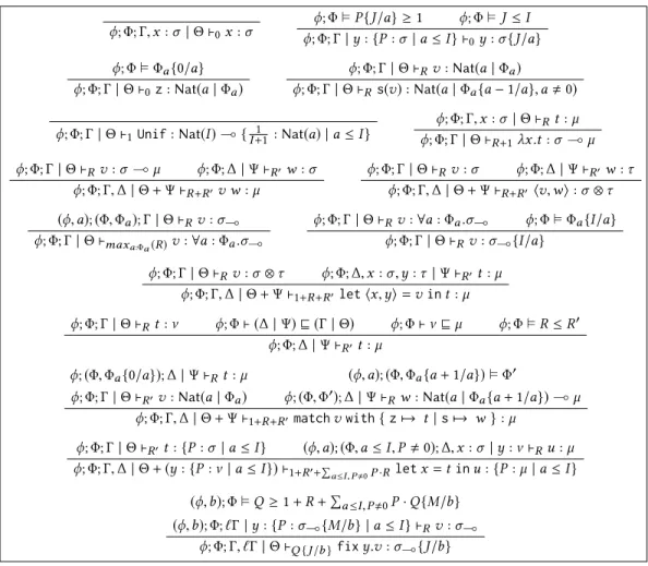
Typing judgments have the formϕ; Φ; Γ | Θ ⊢Rt : µ, with all types present in Γ, Θ and µ valid underϕ; Φ. Active terms are typed with a distribution type µ and values are typed with a linear dependent typeσ. The rational index R is called the weight. It is an indication of the expected runtime of a term and will be used for type soundness.
The type system is given in Figure 6. The axiom rule for recursion context follows the intuition given previously: if the expected number of call toy with type σ {J/a} is greater than 1, then y can be given the typeσ {J/a}. In the rule for the introduction of ∀, the maximum is well-defined and finite since all universal quantification are bounded, as expressed by the definition of validity. Another interesting rule is the one for pattern matching. The typing of the integer and the first case is quite intuitive, but for the second one, in the set of constraintsΦ′,a is not free in Φ′(Φ′ must be valid under(ϕ; Φ)). So, (ϕ, a); (Φ, Φa{a + 1/a}) ⊨ Φ′express thatΦ′is a set of constraint deduced form the fact that at least one integer different from 0 satisfiesΦa. A detailed example will be given later. Finally, in the rule for the fixpoint, the different recursive calls toy are expressed by the valuation type{P : σ⊸{M/b} | a ≤ I }, M being a natural index. And with this description of recursive calls, we ask for an indexQ that satisfies the recurrence relation derived from those recursive calls. This will also be explained in an example.
2.4 Example
We conclude this section with a simple example demonstrating the use of our type system. Let us consider again the term for biased random walk:
rwalk ≜ fix rw.λn.match n with { z 7→ z | s 7→ λn′.rw (s(s(n′))) ⊕2rw n′} . We show that we can give this termrwalk the following type : ⊢ rwalk : Nat(J) ⊸ Nat(0). For the sake of simplicity, we do not detail the weight of this proof, but we will talk briefly about it later. We define the functionBool such that Bool(0) = 0 and Bool(n + 1) = 1. This function is very useful to present index in a simpler form. The first important rule is the one for fixpoint.
b; ⊤; · | rw : {Bool(b)·(a+1)3 :Nat(b+ 1 − 2a) ⊸ Nat(0) | a ≤ 1} ⊢ λn . . . : Nat(b) ⊸ Nat(0)
⊢fix rw.λn . . . : (Nat(b) ⊸ Nat(0)){J/b}
Let us describe this valuation context. Whenb = 0, that is to say when we are in the case rwalk 0, this valuation context expresses that we never callrw. So it means that we stop the recursion. We can see here a reason why we consider valuation and not distribution. Otherwise, whenb , 0, (that is to say in the caserwalk n with n > 0) this valuation context represents the distribution rw : {1
3 :Nat(b+ 1) ⊸ Nat(0); 2
3 :Nat(b − 1) ⊸ Nat(0)}. So it expresses that with probability 1 3, rwalk will be called with the input n + 1 and with probability 2
3 it will be called with the input n − 1. One can remark that in this case, the index M used in the fixpoint describes the reachable states fromb in the Markov chain describing this random walk. From now on, let us call Θ the valuation contextrw : {Bool(b)·(a+1)
3 :Nat(b+ 1 − 2a) ⊸ Nat(0) | a ≤ 1}. We now give the typing for thematch rule:
b; (0 = b); · | Θ ⊢ z : Nat(0) b; ⊤; n : Nat(b) | · ⊢ n : Nat(a | a = b)
(b, a); (a + 1 = b) ⊨ (b ≥ 1)
b; (b ≥ 1); · | Θ ⊢ λn′· · · : Nat(a | a+ 1 = b) ⊸ Nat(0)
ϕ; Φ; Γ, x : σ | Θ ⊢0x : σ ϕ; Φ ⊨ P{J/a} ≥ 1 ϕ; Φ ⊨ J ≤ I ϕ; Φ; Γ | y : {P : σ | a ≤ I } ⊢0y : σ {J/a} ϕ; Φ ⊨ Φa{0/a} ϕ; Φ; Γ | Θ ⊢0z : Nat(a | Φa) ϕ; Φ; Γ | Θ ⊢Rv : Nat(a | Φa) ϕ; Φ; Γ | Θ ⊢Rs(v) : Nat(a | Φa{a − 1/a}, a , 0) ϕ; Φ; Γ | Θ ⊢1Unif : Nat(I) ⊸ { 1 I +1:Nat(a) | a ≤ I } ϕ; Φ; Γ, x : σ | Θ ⊢Rt : µ ϕ; Φ; Γ | Θ ⊢R+1λx.t : σ ⊸ µ ϕ; Φ; Γ | Θ ⊢Rv : σ ⊸ µ ϕ; Φ; ∆ | Ψ ⊢R′w : σ ϕ; Φ; Γ, ∆ | Θ + Ψ ⊢R+R′v w : µ ϕ; Φ; Γ | Θ ⊢Rv : σ ϕ; Φ; ∆ | Ψ ⊢R′w : τ ϕ; Φ; Γ, ∆ | Θ + Ψ ⊢R+R′⟨v, w⟩ : σ ⊗ τ (ϕ, a); (Φ, Φa);Γ | Θ ⊢Rv : σ⊸
ϕ; Φ; Γ | Θ ⊢maxa:Φa(R)v : ∀a : Φa.σ⊸
ϕ; Φ; Γ | Θ ⊢Rv : ∀a : Φa.σ⊸ ϕ; Φ ⊨ Φa{I/a} ϕ; Φ; Γ | Θ ⊢Rv : σ⊸{I/a} ϕ; Φ; Γ | Θ ⊢Rv : σ ⊗ τ ϕ; Φ; ∆, x : σ,y : τ | Ψ ⊢R′t : µ ϕ; Φ; Γ, ∆ | Θ + Ψ ⊢1+R+R′let ⟨x,y⟩ = v in t : µ ϕ; Φ; Γ | Θ ⊢Rt : ν ϕ; Φ ⊢ (∆ | Ψ) ⊑ (Γ | Θ) ϕ; Φ ⊢ ν ⊑ µ ϕ; Φ ⊨ R ≤ R′ ϕ; Φ; ∆ | Ψ ⊢R′t : µ ϕ; (Φ, Φa{0/a}); ∆ | Ψ ⊢Rt : µ ϕ; Φ; Γ | Θ ⊢R′v : Nat(a | Φa) (ϕ, a); (Φ, Φa{a + 1/a}) ⊨ Φ′ ϕ; (Φ, Φ′);∆ | Ψ ⊢ Rw : Nat(a | Φa{a + 1/a}) ⊸ µ ϕ; Φ; Γ, ∆ | Θ + Ψ ⊢1+R+R′match v with { z 7→ t | s 7→ w } : µ ϕ; Φ; Γ | Θ ⊢R′t : {P : σ | a ≤ I } (ϕ, a); (Φ, a ≤ I, P , 0); ∆, x : σ | y : ν ⊢Ru : µ ϕ; Φ; Γ, ∆ | Θ + (y : {P : ν | a ≤ I }) ⊢1+R′+Í a ≤I , P ,0P ·Rlet x = t in u : {P : µ | a ≤ I } (ϕ,b); Φ ⊨ Q ≥ 1 + R + Ía ≤I,P ,0P · Q{M/b} (ϕ,b); Φ; ℓΓ | y : {P : σ⊸{M/b} | a ≤ I } ⊢Rv : σ⊸ ϕ; Φ; Γ, ℓΓ | Θ ⊢Q {J /b }fix y.v : σ⊸{J/b}
Fig. 6. Type System for dℓRPCF
The variablen has type Nat(b). Thus, when we know that n is a successor, in the second branch of the match, we can prove thatb ≥ 1. This is expressed by (b, a); (a + 1 = b) ⊨ (b ≥ 1). So we can use this hypothesis(b ≥ 1) in the second branch of the match. Remark also that when b ≥ 1, the type Nat(a | a+ 1 = b) is equivalent to Nat(b − 1).
For the sake of simplicity, we now show informally how to use the probabilistic choice⊕2. This operator (or more precisely thelet operator) allow us to "split" the valuation context according to the probabilities of each branch of this probabilistic choice. Thus, the valuation contextΘ can be split into two valuation contextΨ1andΨ2ifΘ correspond to the convolution {1
3 :Ψ1; 2 3 :Ψ2}. AsΘ representsrw : {1 3 :Nat(b+ 1) ⊸ Nat(0); 2
3 :Nat(b − 1) ⊸ Nat(0)} we can take
Ψ1 = rw : {1 : Nat(b + 1) ⊸ Nat(0)} and Ψ2 = rw : {1 : Nat(b − 1) ⊸ Nat(0)} used to type rw (s(s(n′))) andrw n′
respectively. Formally, the intuition given above correspond to a subtyping rule for valuation context.
Finally, for the weight of this proof, the subterm
λn.match n with { z 7→ z | s 7→ λn′.rw (s(s(n′
can be typed with a constant weight equals to 7. Thus, the fixpoint rule gives us the inequation b; ⊤ ⊨ Q ≥ 8 + Ía ≤1Bool(b)·(a+1)3 ·Q{b + 1 − 2a/b}. That is to say,
⊨ Q {0/b} ≥ 8 and b; (b ≥ 1) ⊨ Q ≥ 8 +1
3·Q{b + 1/b} + 2
3·Q{b − 1/b}. This relation is thus very close to the expression of the expected time of a random walk. A solution of this inequation is Q = 8(3b + 1).
3 TYPE SOUNDNESS
We now show the type soundness of our calculus. For this, we show that the weight described in the type system in Figure 6 is a bound on the expected runtime of a term. As we proved that they are equivalent, we work with the alternative subtyping rule.
3.1 Weakening, Contraction and Index Substitution
We first present general proprieties on indexes, types and typing derivation. Especially, we show that the use of a set of index variableϕ and a set of constraint Φ corresponds intuitively to a universal quantification over all variableϕ that satisfies Φ.
Lemma 3.1 (Weakening). Letϕ; Φ be a set of index variables and constraints. Let ϕ′be a set of index variables disjoint fromϕ. Let Φ′be a set of constraint valid under (ϕ, ϕ′);Φ.
(1)Ifϕ; Φ ⊨ A R B then (ϕ, ϕ′); (Φ, Φ′) ⊨ A R B. (2)Ifϕ; Φ ⊢ ζ valid then (ϕ, ϕ′);Φ, Φ′⊢ζ valid. (3)Ifϕ; Φ ⊢ ζ ⊑ ξ then (ϕ, ϕ′); (Φ, Φ′) ⊢ζ ⊑ ξ .
(4)Ifϕ; Φ; Γ | Θ ⊢R t : µ then for all ϕ′, Φ′, Γ′such that the concatenation Γ, Γ′are defined, we have (ϕ, ϕ′); (Φ, Φ′);Γ, Γ′ | Θ ⊢R t : µ. Moreover, if Θ = ∅ then for any Θ′
we have (ϕ, ϕ′); (Φ, Φ′);Γ, Γ′|Θ′⊢
Rt : µ
The first point comes from the definition of⊨. Then, points 2,3 and 4 are proved by induction on the definition of validity, definition of subtyping and typing derivation. All cases are direct.
Lemma 3.2 (Constraint Contraction). Let (ϕ; Φ) be a set of index variables and constraints. Let C be a constraint on ϕ such that ϕ; Φ ⊨ C.
(1)Ifϕ; (Φ,C) ⊨ A R B then ϕ; Φ ⊨ A R B. (2)Ifϕ; (Φ,C) ⊢ ζ valid then ϕ; Φ ⊢ ζ valid. (3)Ifϕ; (Φ,C) ⊢ ζ ⊑ ξ then ϕ; Φ ⊢ ζ ⊑ ξ .
(4)Ifϕ; (Φ,C); Γ | Θ ⊢Rt : µ then ϕ; Φ; Γ | Θ ⊢Rt : µ.
Again, the first point comes from the definition of⊨ and the other ones are proved by induction. All cases are rather direct using the weakening lemma. This shows that set of constraints work as expected: if a constraint does not add any information, then it can be removed. Finally, we show that we can instantiate index variables inϕ.
Lemma 3.3 (Index Substitution). Let (ϕ, a); Φ be a set of index variables and constraints. Let K be a natural index with free variables inϕ.
(1)For a valuationρ : ϕ → N, we have for all index A with free variables in (ϕ, a), JA{K /a }Kρ =JAKρ[a7→JK Kρ]. Moreover,ρ ⊨ Φ{K/a} iff ρ[a 7→JK Kρ] ⊨ Φ. (2)If (ϕ, a); Φ ⊨ A R B then ϕ; Φ{K/a} ⊨ (A{K/a}) R (B{K/a}).
(3)If (ϕ, a); Φ ⊢ ζ valid then ϕ; Φ{K/a} ⊢ ζ {K/a} valid. (4)If (ϕ, a); Φ ⊢ ζ ⊑ ξ then ϕ; Φ{K/a} ⊢ ζ {K/a} ⊑ ξ {K/a}.
The first point comes from the definition of
J·Kρ. Then, the other points are proved by induction. This is rather direct using the fact that, for all indexI with free variables in (ϕ, a,b), J with free variable in(ϕ, a) and K with free variable in ϕ, we have I {J/b}{K/a} = I {K/a}{J {K/a}/b}. 3.2 Proprieties of Values and Substitution Lemmas
We now present the usual substitution lemmas in the case of our calculus. In order to do that, we show the rule of values in our calculus.
Lemma 3.4 (Progress). Letϕ; Φ; · | · ⊢Rt : µ. Then t is normal for → if and only if t is a value v. This is not surprising as it correspond exactly to the Lemma 1.1 in the simple type system. A particular kind of values that interest us are integers values and their type. We can show that the typeNat(a | Φa) is indeed the set of integersn such that Φa{n/a}.
Lemma 3.5 (Integers Values). Letv be a value such that ϕ; Φ; · | · ⊢Rv : Nat(a | Φa), thenv = n for some integern and ϕ; Φ ⊨ Φa{n/a}. Reciprocaly, for any n such that ϕ; Φ ⊨ Φa{n/a}, we can give the typingϕ; Φ; · | · ⊢0n : Nat(a | Φa).
This is proved by induction on the typing rule for the first proposition. The second proposition is rather direct. Then, we work on the definition ofelements. Intuitively, elements describe the elements of a type, and subtyping correspond to inclusion between types. Thus, we obtain the following lemma:
Lemma 3.6 (Subtyping and Elements). Letσ, τ be valid types under ϕ; Φ such that ϕ; Φ ⊢ σ ⊑ τ . Then, we haveelements(σ) = ϕ′;Φσ;σ′andelements(τ ) = ϕ′;Φτ;τ′such that (ϕ, ϕ′); (Φ, Φσ) ⊨ Φτ and (ϕ, ϕ′); (Φ, Φσ) ⊢σ′⊑τ′
.
The fact that we can give the same set of index variableϕ′for the twoelements is just a matter of renaming, asσ and τ have the same form by subtyping. We prove this by induction on σ (and τ ). Ifσ is an arrow type, this is direct by definition of elements. If σ is a tensor type, this is rather direct by induction hypothesis, by definition of subtyping for tensor and by weakening. Ifσ is Nat(a | Φa) for someΦa, then this is exactly the definition of subtyping of integers. We can now show the link betweenelements and typed values.
Lemma 3.7 (values and Elements). Letv be a value such that ϕ; Φ; · | · ⊢R v : σ. Suppose thatelements(σ) = a; Φa;τ . Then there exists an instantiation I of a valid under ϕ; Φ such that ϕ; Φ ⊨ Φa{I/a} and ϕ; Φ; · | · ⊢Rv : τ {I/a}.
We prove this by induction on the typeσ. If σ is an arrow type then this is direct by definition ofelements. Let us detail the two other cases.
• Nat: Ifσ = Nat(a | Φa). By definition,elements(σ) = a; Φa;Nat(a). By Lemma 3.5, v= n for some integern and ϕ; Φ ⊨ Φa{n/a}. Thus, we can take n for instantiation of a and again by Lemma 3.5, asϕ; Φ ⊨ (a′= n){n/a′}, we can give the typingϕ; Φ; · | · ⊢0n : Nat(a){n/a}. This concludes the case.
• Tensor: Ifσ = σ0⊗σ1, then the typingϕ; Φ; · | · ⊢Rv : σ0⊗σ1can be given a particular form. Indeed, by reflexivity and transitivity of subtyping, any chain of subtyping rule is equivalent to exactly one subtyping rule. Asσ is not an arrow type, subtyping is the only possible non syntax-directed rule, and the only way to give a value a tensor type is if this value is a tensor of value and by using a tensor introduction rule. Thus, we have the typing
ϕ; Φ; · | · ⊢R0v0:τ0 ϕ; Φ; · | · ⊢R1v1:τ1 ϕ; Φ; · | · ⊢R0+R1 ⟨v0,v1⟩ :τ0⊗τ1
ϕ; Φ ⊨ R0+ R1≤R
ϕ; Φ ⊢ τ0⊗τ1⊑σ0⊗σ1
Let us poseelements(τ0)= a0;Φ0;τ ′
0andelements(τ1)= a1;Φ1;τ ′
1. By induction hypothesis, there exists instantiationsI0ofa0andI1ofa1such thatϕ; Φ ⊨ Φ0{I0/a0} and
ϕ; Φ ⊨ Φ1{I1/a1} andϕ; Φ; · | · ⊢R0 v0 : τ
′
0{I0/a0} andϕ; Φ; · | · ⊢R1 v1 : τ
′
1{I1/a1}. By Lemma 3.6, we haveelements(σ0⊗σ1)= (a0, a1);Φσ;σ
′such that(ϕ, a 0, a1); (Φ, Φ0, Φ1) ⊨ Φσ and(ϕ, a0, a1); (Φ, Φ0, Φ1) ⊢τ ′ 0 ⊗τ ′ 1 ⊑σ
′. Thus, by Lemma 3.3 and Lemma 3.2, we obtain ϕ; Φ ⊨ Φσ{I0, I1/a0, a1} andϕ; Φ ⊢ (τ ′ 0 ⊗τ ′ 1){I0, I1/a0, a1} ⊑σ ′{I 0, I1/a0, a1}. By subtyping, from the proofϕ; Φ; · | · ⊢R
0+R1 ⟨v0,v1⟩ : (τ
′ 0⊗τ
′
1){I0, I1/a0, a1} we can obtain the proof ϕ; Φ; · | · ⊢R ⟨v0,v1⟩ :σ′{I0, I1/a0, a1}, and this concludes the case.
We can now present the substitution lemmas for our calculus. In our reduction rules, the only terms that are used in a substitution are values, thus we can restrict substitution lemmas to values. There are two kind of substitution in this calculus. First, a standard substitution corresponding to non-monadic types.
Lemma 3.8 (Substitution Lemma for Linear Contexts). Suppose that we have a proof ϕ; Φ; Γ, x : σ | Θ ⊢Rt : µ and a proof ϕ; Φ; · | · ⊢R′v : σ then we can derive the proof
ϕ; Φ; Γ | Θ ⊢R+R′t[x := v] : µ
The lemma is essentially a consequence of linearity of the type system. In order to prove this we distinguish two cases. Ifσ = Nat(a | Φa) for someΦa, thenx is duplicable. However, by the previous lemma,v = n for some n ∈ N. So we have a proof ϕ; Φ; · | · ⊢0v : Nat(a | Φa). This weight equals to 0 implies that we haveϕ; Φ; Γ | Θ ⊢Rt[x := v] : µ. Otherwise, x : σ appears in only one context in a concatenationΓ, ∆ and we can use the induction hypothesis on the branches where x appears.
The other substitution is the one for valuation contexts, in which variable are give a dynamic valuation type. For this let us first give a notation for indexes that we will use in the proof.
Definition 3.9 (Extract). Letϕ be a set of index variables, a < ϕ, and I an index with free variables inϕ and J an index with free variable in (ϕ, a). We define ext(a, I, J) as an index with free variables inϕ such that ϕ; Ía ≤I J , 0 ⊨ (ext(a, I, J) ≤ I) ∧ (J {ext(a, I, J)/a} , 0) and
(ϕ, a); (a ≤ I, J = 0) ⊨ ext(a, I, J) = 0. Intuitively, for ρ : ϕ → N, whenJÍ
a ≤I JKρ is non-null, then Jex t (a, I , J )Kρis an integern smaller thanJI Kρsuch thatJJ Kρ[a7→n]is non-null. Note that with this definition, there is not a unique choice for
Jex t (a, I , J )Kρ, but when we do not say otherwise, we just take the smaller integer verifying those conditions.
Lemma 3.10 (Substitution Lemma for Valuation Contexts). Suppose that
ϕ; Φ; Γ | y : {P : σ | a ≤ I } ⊢R′ t : µ and (ϕ, a); (Φ, a ≤ I, P , 0); · | · ⊢R v : σ. Then
ϕ; Φ; Γ | · ⊢R′+Í
a ≤I , P ,0P ·R t[y := v] : µ.
Proof. We prove this by induction on the typing oft. We detail some non-trivial cases. • Axiom: Suppose we have the typing :
ϕ; Φ ⊨ P{J/a} ≥ 1 ϕ; Φ ⊨ J ≤ I
ϕ; Φ; Γ | y : {P : σ | a ≤ I } ⊢0y : σ {J/a}
And suppose(ϕ, a); (Φ, a ≤ I, P , 0); · | · ⊢Rv : σ. By Lemma 3.3, we obtain
ϕ; (Φ, J ≤ I, P {J/a} , 0); · | · ⊢R {J /a }v : σ {J/a}. As ϕ; Φ ⊨ J ≤ I and ϕ; Φ ⊨ P{J/a} ≥ 1, by Lemma 3.2, we obtainϕ; Φ; · | · ⊢R {J /a }v : σ {J/a}. By weakening, we obtain
ϕ; Φ; Γ | · ⊢R {J /a }y[y := v] : σ {J/a}. As ϕ; Φ ⊨ 1 ≤ P{J/a} and ϕ; Φ ⊨ J ≤ I, we have ϕ; Φ ⊨ R{J/a} ≤ (P · R){J/a} ≤ Ía ≤I,P ,0P · R and we can conclude this case by subtyping. • Application: Suppose we have the typing :
ϕ; Φ; Γ | y : {P : σ | a ≤ I } ⊢R0w0
:σ ⊸ µ ϕ; Φ; ∆ | y : {Q : σ | a ≤ I } ⊢R
1w1 :σ ϕ; Φ; Γ, ∆ | y : {(P + Q) : σ | a ≤ I } ⊢R0+R1w0w1:µ
And suppose(ϕ, a); (Φ, a ≤ I, P + Q , 0); · | · ⊢Rv : σ. By weakening, we obtain (ϕ, a); (Φ, a ≤ I, P + Q , 0, P , 0); · | · ⊢Rv : σ, and then by contraction, we obtain (ϕ, a); (Φ, a ≤ I, P , 0); · | · ⊢Rv : σ. By induction hypothesis, we have
ϕ; Φ; Γ | · ⊢R0+Ía ≤I , P ,0P ·Rw0[y := v] : σ ⊸ µ. In the same way, we obtain
ϕ; Φ; ∆ | · ⊢R1+Ía ≤I , Q ,0Q ·R w1[y := v] : σ. Thus, by using the application rule, we obtain
ϕ; Φ; Γ, ∆ | · ⊢R0+R1+Ía ≤I , (P+Q),0(P +Q)·R(w0w1)[y := v] : µ. The same method can be used for
any rule that uses this concatenationΘ + Ψ such as tensor introduction, tensor elimination and pattern matching.
• Subtyping : Suppose we have the following derivation tree :
ϕ; Φ; ∆ | y : {Q : τ | b ≤ J } ⊢R0t : ν
ϕ; Φ ⊢ ν ⊑ µ, Γ ⊑ ∆ ϕ; Φ ⊨ R0≤R1
ϕ; Φ ⊢ {P : σ | a ≤ I } ⊑ {Q : τ | b ≤ J } ϕ; Φ; Γ | y : {P : σ | a ≤ I } ⊢R′t : µ
And we have(ϕ, a); (Φ, a ≤ I, P , 0); · | · ⊢Rv : σ. By definition of subtyping, there exists a rational indexS such that ϕ; Φ ⊢ S ◁⊑⟨{P : σ | a ≤ I }&{Q : τ | b ≤ J }⟩. By weakening, we obtain the proof(ϕ, a,b); (Φ, a ≤ I, P , 0,b ≤ J,Q , 0, S , 0); · | · ⊢Rv : σ. By subtyping, we have(ϕ, a,b); (Φ, a ≤ I, P , 0,b ≤ J,Q , 0, S , 0); · | · ⊢Rv : τ . Let us call H = ext(a, I, S), withH chosen such that R{H/a} is minimal. By lemma 3.3, we obtain :
(ϕ,b); (Φ, H ≤ I, P {H/a} , 0,b ≤ J,Q , 0, S{H/a} , 0); · | · ⊢R {H /a } v : τ . Moreover, by definition we have(ϕ,b); (Q , 0) ⊨ (H ≤ I) ∧ (S{H/a} , 0).
As(ϕ, a,b); (Φ, a ≤ I,b ≤ J, S , 0) ⊨ P , 0, we also have
(ϕ,b); (Φ, H ≤ I,b ≤ J, S{H/a} , 0) ⊨ P{H/a} , 0. Thus, by contraction, we obtain : (ϕ,b); (Φ,b ≤ J, Q , 0); · | · ⊢R {H /a }v : τ . Moreover,
(ϕ,b); (Φ,b ≤ J, Q , 0) ⊨ R{H/a} ≤ Ía ≤I,P ,0S ·RQ since(Φ,b); (Φ,b ≤ J) ⊨ Q = Ía ≤IS and by definition ofH, (ϕ,b, a); (Φ,b ≤ J, Q , 0, a ≤ I, S , 0) ⊨ R{H/a} ≤ R. Thus, we have(ϕ,b, a); (Φ,b ≤ J, Q , 0, a ≤ I) ⊨ S · R{H/a} ≤ S · R. So, in conclusion, we obtain(ϕ,b); (Φ,b ≤ J, Q , 0); · | · ⊢Í
a ≤I , P ,0S ·RQ v : τ . By induction hypothesis, we obtain
ϕ; Φ; ∆ | · ⊢R0+Íb ≤ J , a ≤I , P ,0,Q ,0S ·R t[y := v] : ν. Furthermore, we have ϕ; Φ ⊨ R0 ≤ R1
andϕ; Φ ⊨ Íb ≤J,a ≤I,Q,0,P,0S · R = Ía ≤I,P ,0P · R. So with a subtyping rule, we obtain ϕ; Φ; Γ | · ⊢R1+Ía ≤I , P ,0P ·R t[y := v] : µ, and this concludes this case.
• Let : Suppose we have the typing
ϕ; Φ; Γ | Θ ⊢S′t : {P : τ | a ≤ I } (ϕ, a); (Φ, a ≤ I, P , 0); ∆, x : τ | y : ν ⊢Su : µ ϕ; Φ; Γ, ∆ | Θ + (y : {P : ν | a ≤ I }) ⊢1+S′+Í
a ≤I , P ,0P ·S let x = t in u : {P : µ | a ≤ I }
We considerΘ = ∅. Let us note ν = {Q : σ | b ≤ J }. By definition of convolution, suppose given a proof(ϕ, c); (Φ, c ≤ Ía ≤I(J + 1), (P · Q){πa
1(I, J, c)/a}{π a 2(I, J, c)/b} , 0); · | · ⊢Rv : σ {πa 1(I, J, c)/a}{π a
2(I, J, c)/b}. By weakening and substitution we obtain (ϕ, a′,b′); (Φ, a′⋆a
I, Jb′ ≤ Ía ≤I(J + 1), a′ ≤ I,b′ ≤ J {a′/a}, (P · Q){a′/a}{b′/b} , 0); · | · ⊢R {a′⋆a
I , Jb′/c }v : σ {a
′/a}{b′/b}. Let us call J′= J {a′/a}. By renaming and contraction: (ϕ, a,b); (Φ, a ≤ I,b ≤ J, P , 0,Q , 0); · | · ⊢R {a⋆a′
I , J ′b/c }v : σ. By induction hypothesis, we
obtain(ϕ, a); (Φ, a ≤ I, P , 0); ∆, x : τ | · ⊢
S+Íb ≤ J , Q ,0Q ·R {a⋆a′I , J ′b/c }u[y := v] : µ. Then, using
the rule forlet, we obtain the proof ϕ; Φ; Γ, ∆ | · ⊢1+S′+Í
a ≤I , P ,0P (S+Íb ≤ J , Q ,0Q ·R {a⋆I , J ′a′ b/c })
(let x = t in u)[y := v] : {P : µ | a ≤ I }. Furthermore,
ϕ; Φ ⊨ Ía ≤I,(P ·Q),0,b ≤JP · Q · R{a ⋆a
′
I, J′b/c} = Íc ≤Í
a ≤I(J +1),(P ·Q){π1a(I, J,c)/a }{π a
2(I, J,c)/b },0R ·
(P ·Q){πa
1(I, J, c)/a}{π a
2(I, J, c)/b}, and this concludes the proof for this case. The case Θ , ∅ is similar.
3.3 Generation Lemma and Subject Reduction
Now, in order to give the subject reduction, we first need to consider the difficult case of values with an arrow type. Indeed, with the rule for introduction and elimination of quantification, a typing derivation for a value with an arrow type is not always a subtyping rule below a syntax-directed rule, such as theλ-abstraction rule, the fixpoint rule or the rule for Unif. Trying to explain what this possible chain of subtyping, introduction of quantification and elimination of quantification does is the goal of the following generation lemma.
Lemma 3.11 (Generation Lemma). Suppose given a proof
π
ϕ; Φ; · | · ⊢Rv : σ ⊸ µ ϕ; Φ; · | · ⊢R′w : σ
ϕ; Φ; · | · ⊢R+R′v w : µ
Then in the canonical representation ofπ, that is to say π in which before each non-subtyping rule we have exactly one subtyping rule, for any (ϕ,b); (Φ, Φb); · | · ⊢R0v : ∀a : Φa.σ0⊸ µ0, there exists
an instantiationIb, Ia ofb, a valid under ϕ; Φ such that ϕ; Φ ⊨ Φb{Ib/b}, ϕ; Φ ⊨ Φa{Ib, Ia/b, a}, ϕ; Φ ⊢ µ0{Ia, Ib/a,b} ⊑ µ and we have a proof ϕ; Φ; · | · ⊢R′ w : σ0{Ia, Ib/a,b}. Furthermore,
ϕ; Φ ⊨ R0{Ib/b} ≤ R.
Proof. We prove this lemma by induction, from bottom to top, on the canonical representation of π. We first show that any subproof in the canonical representation of π before the syntax-directed rule has indeed the form(ϕ, ϕ′); (Φ, Φ′); · | · ⊢R
0v : σ⊸for someϕ
′, Φ′, σ
⊸. Let us ignore the index R0for this first proposition as it does not matter here.
• Base case : The base case, as the induction goes from bottom to top, isϕ; Φ; · | · ⊢ v : σ ⊸ µ given in the previous typing. This has indeed to good form.
• Elimination of quantification. Let suppose that the bottom proof has indeed the form (ϕ, ϕ′); (Φ, Φ′); · | · ⊢
R0v : σ⊸. Thus we have the typing: (ϕ, ϕ′); (Φ, Φ′); · | · ⊢v : ∀a : Φa.τ⊸ (ϕ, ϕ′); (Φ, Φ′) ⊨ Φa{I/a}
(ϕ, ϕ′); (Φ, Φ′); · | · ⊢v : τ⊸{I/a} (ϕ, ϕ′); (Φ, Φ′) ⊢τ⊸{I/a} ⊑ σ⊸
(ϕ, ϕ′); (Φ, Φ′); · | · ⊢v : σ ⊸
So we have indeed only typing with the form(ϕ, ϕ′); (Φ, Φ′); · | · ⊢v : σ⊸for someϕ′, Φ′, σ⊸. • Other cases : Introduction of quantification works in the same way: it only add new variables and constraints so it does not contradict the form(ϕ, ϕ′); (Φ, Φ′); · | · ⊢v:σ⊸. The other cases are the syntax directed-rule. Note that for value with arrow types, there is exactly 3 possibilities :λ- abstraction, fixpoint and Unif, and again those this does not contradict the form given in the theorem.
Now that we know exactly the shape of those proofs. We can prove the proposition.
• Base case : The base case is direct, forϕ; Φ; · | · ⊢Rv : σ ⊸ µ, a = b = ∅ thus the instantiation is the null instantiation, and we have indeedϕ; Φ ⊢ µ ⊑ µ and a proof ϕ, Φ; · | · ⊢R′ w : σ.
Furthermore,ϕ, Φ ⊨ R ≤ R.
(ϕ,b); (Φ, Φb); · | · ⊢R0v : ∀c0:Φ0.(∀c : Φc.τ0⊸ ν0) (ϕ,b); (Φ, Φb) ⊨ Φ0{I/c0} (ϕ,b); (Φ, Φb); · | · ⊢R 0v : (∀c : Φc.τ0⊸ ν0){I/c0} (ϕ,b); (Φ, Φb) ⊢ (∀c : Φc.τ0⊸ ν0){I/c0} ⊑∀a : Φa.σ0⊸ µ0 (ϕ,b); (Φ, Φb); · | · ⊢R 1v : ∀a : Φa.σ0⊸ µ0
With(ϕ,b); (Φ, Φb) ⊨ R0≤R1. By induction hypothesis, there exists an instantiationIb, Iaof b, a such that ϕ; Φ ⊨ Φb{Ib/b}, ϕ; Φ ⊨ Φa{Ia, Ib/a,b}, ϕ; Φ ⊢ µ0{Ia, Ib/a,b} ⊑ µ and we have a proofϕ; Φ; · | · ⊢R′w : σ0{Ia, Ib/a,b}. Furthermore, ϕ; Φ ⊨ R1{Ib/b} ≤ R. By definition of subtyping, if we denoteelements(σ0)= d; Φd, σ1, then there existsIcsuch that
(ϕ,b, a,d); (Φ, Φb, Φa, Φd) ⊨ Φc{I/c0}{Ic/c} (ϕ,b, a,d); (Φ, Φb, Φa, Φd) ⊢σ1⊑τ0{I/c0}{Ic/c} (ϕ,b, a,d); (Φ, Φb, Φa, Φd) ⊢ν0{I/c0}{Ic/c} ⊑ µ0
Thus, by index substitution, contraction, and definition ofelements, we have elements(σ0{Ia, Ib/a,b}) = d; Φd{Ia, Ib/a,b}; σ1{Ia, Ib/a,b}
(ϕ,d); (Φ, Φd) ⊨ Φc{Ib/b}{I {Ib/b}/c0}{Ic{Ia, Ib/a,b}/c}
(ϕ,d); (Φ, Φd) ⊢σ1{Ia, Ib/a,b} ⊑ τ0{Ib/b}{I {Ib/b}/c0}{Ic{Ia, Ib/a,b}/c} (ϕ,d); (Φ, Φd) ⊢ν0{Ib/b}{I {Ib/b}/c0}{Ic{Ia, Ib/a,b}/c} ⊑ µ0{Ia, Ib/a,b}
By Lemma 3.7, there exists an instantiationIdofd such that ϕ; Φ ⊨ Φd{Ia, Ib/a,b}{Id/d} and we have a proofϕ; Φ; · | · ⊢R′w : σ1{Ia, Ib/a,b}{Id/d}. Let us give the following notation
Jc = Ic{Ia, Ib, Id/a,b,d} and J = I {Ib/b}. Again by index substitution and contraction : ϕ; Φ ⊨ Φ0{Ib/b}{J/c0}
ϕ; Φ ⊨ Φc{Ib/b}{J/c0}{Jc/c}
ϕ; Φ ⊢ σ1{Ia, Ib/a,b}{Id/d} ⊑ τ0{Ib/b}{J/c0}{Jc/c} ϕ; Φ ⊢ ν0{Ib/b}{J/c0}{Jc/c} ⊑ µ0{Ia, Ib/a,b} ⊑ µ
So, the instantiation ofb, c0, c is given by Ib, J, Jc, thenϕ; Φ ⊢ ν0{Ib/b}{J/c0}{Jc/c} ⊑ µ is given by transitivity of subtyping, and the proofϕ; Φ; · | · ⊢R′w : τ0{Ib/b}{J/c0}{Jc/c} is
given by subtyping. Finally,ϕ, Φ ⊨ R0{Ib/b} ≤ R by index substitution and transitivity of ≤. This concludes this case.
• Introduction of quantification : Suppose we have the typing
(ϕ,b, c0); (Φ, Φb, Φ0); · | · ⊢R 0v : ∀c : Φc.τ0⊸ ν0 (ϕ,b); (Φ, Φb); · | · ⊢max c0:Φ0(R0)v : ∀c0 :Φ0.(∀c : Φc.τ0⊸ ν0) (ϕ,b); (Φ, Φb) ⊢∀c0:Φ0.(∀c : Φc.τ0⊸ ν0) ⊑∀a : Φa.σ0⊸ µ0 (ϕ,b); (Φ, Φb); · | · ⊢R 1v : ∀a : Φa.σ0⊸ µ0 With(ϕ,b); (Φ, Φb) ⊨ maxc
0:Φ0(R0) ≤R1. By induction hypothesis, there exists an
instantia-tionIb, Iaofb, a such that ϕ; Φ ⊨ Φb{Ib/b}, ϕ; Φ ⊨ Φa{Ia, Ib/a,b}, ϕ; Φ ⊢ µ0{Ia, Ib/a,b} ⊑ µ and we have a proofϕ; Φ; · | · ⊢R′w : σ0{Ia, Ib/a,b}. Furthermore, ϕ; Φ ⊨ R1{Ib/b} ≤ R. By
definition of subtyping, if we denoteelements(σ0)= d; Φd, σ1, then there existsI, Icsuch that
(ϕ,b, a,d); (Φ, Φb, Φa, Φd) ⊨ Φ0{I/c0} (ϕ,b, a,d); (Φ, Φb, Φa, Φd) ⊨ Φc{I/c0}{Ic/c} (ϕ,b, a,d); (Φ, Φb, Φa, Φd) ⊢σ1⊑τ0{I/c0}{Ic/c} (ϕ,b, a,d); (Φ, Φb, Φa, Φd) ⊢ν0{I/c0}{Ic/c} ⊑ µ0
and we have a proofϕ; Φ; · | · ⊢R′w : σ1{Ia, Ib/a,b}{Id/d}. Let us give the following notation
Jc = Ic{Ia, Ib, Id/a,b,d} and J = I {Ia, Ib, Id/a,b,d}. We obtain : ϕ; Φ ⊨ Φ0{Ib/b}{J/c0}
ϕ; Φ ⊨ Φc{Ib/b}{J/c0}{Jc/c}
ϕ; Φ ⊢ σ1{Ia, Ib/a,b}{Id/d} ⊑ τ0{Ib/b}{J/c0}{Jc/c} ϕ; Φ ⊢ ν0{Ib/b}{J/c0}{Jc/c} ⊑ µ0{Ia, Ib/a,b} ⊑ µ
And we can concludes in the same way as the previous case. The only difference, is for the weight. We have(ϕ,b); (Φ, Φb) ⊨ maxc
0:Φ0(R0) ≤R1, and so, we have
ϕ; Φ ⊨ maxc
0:Φ0{Ib/b }(R0{Ib/b}) ≤ R1{Ib/b} ≤ R And by definition of maximum, we obtain
ϕ; Φ ⊨ R0{Ib/b}{J/c0} ≤maxc
0:Φ0{Ib/b }
(R0{Ib/b}) ≤ R1{Ib/b} ≤ R, and this concludes this case.
• Other cases : The other cases are for the syntax-directed rule, for exampleλ-abstraction. In this case, the typing would be :
(ϕ,b); (Φ, Φb);x : τ0| · ⊢R0t : ν0 (ϕ,b); (Φ, Φb); · | · ⊢R
0+1λx.t : τ0⊸ ν0 (ϕ,b); (Φ, Φb) ⊢τ0⊸ ν0⊑∀a : Φa.σ0⊸ µ0
(ϕ,b); (Φ, Φb); · | · ⊢R1v : ∀a : Φa.σ0⊸ µ0
And so we only need to prove our propriety for the subtyping rule. And this works in the same way as the previous cases, in which we considered subtyping and another rule. This is the same idea for all other syntax-directed rule.
This concludes the proof for the generation lemma. We can now give the main theorem of subject reduction.
Theorem 3.12 (Subject Reduction). Ifϕ; Φ; · | · ⊢Rt : {P : σ | a ≤ I } and t → {pi :ti |i ∈ I} (withpi > 0 for all i), then for all i ∈ I, there exists valid rational indexes PiandRi such that ϕ; Φ; · | · ⊢Ri ti :µi withϕ; Φ ⊢ µi ⊑ {Pi :σ | a ≤ I } and (ϕ, a); (Φ, a ≤ I) ⊨ P = Íi ∈Ipi ·Pi and ϕ; Φ ⊨ R ≥ 1 + Íi ∈Ipi ·Ri.
Proof. We prove this by induction on the reductiont → {pi :ti |i ∈ I}. First, we show that it is sufficient to prove the subject reduction for a typing derivation fort that does not start with a subtyping rule. Indeed, suppose the subject reduction proved for such typing derivations, and supposeϕ; Φ; · | · ⊢Rt : {P : σ | a ≤ I } with t → {pi :ti |i ∈ I}. Suppose the typing derivation has the form:
ϕ; Φ ⊢ R′≤R
ϕ; Φ; · | · ⊢R′t : {P′:σ′|a′≤I′} ϕ; Φ ⊢ {P′:σ′|a′≤I′} ⊑ {P : σ | a ≤ I } ϕ; Φ; · | · ⊢Rt : {P : σ | a ≤ I }
By subject reduction, we have for alli ∈ I, ϕ; Φ; · | · ⊢R′
i t : µ with ϕ; Φ ⊢ µ ⊑ {P
′
i :σ′|a′≤I′} and(ϕ, a′); (Φ, a′≤I′) ⊨ P′= Íi ∈Ipi·Pi′andϕ; Φ ⊨ R′≥ 1+ Íi ∈Ipi·Ri′. Let us callS the rational index in the coupling given in the proof. We define the rational indexSi by
Si = i f (P′= 0) then 0 else S ·Pi′
P′ and we definePi = Ía′≤I′Si. We have then easily ϕ; Φ ⊢ Si◁⊑⟨{Pi′:σ′|a′≤I′}&{Pi :σ | a ≤ I }⟩. Thus,
ϕ; Φ ⊢ µ ⊑ {P′
i :σ′|a′≤I′} ⊑ {Pi :σ | a ≤ I }. Moreover
(ϕ, a); (Φ, a ≤ I) ⊨ Íi ∈Ipi·Pi = P using the fact that (ϕ, a, a′); (Φ, a ≤ I, a′≤I′) ⊨Í
i ∈Ipi·Si = S. Moreover,ϕ; Φ ⊨ R ≥ R′≥ 1+ Íi ∈Ipi·Ri′. This concludes the subject reduction in the case of a subtyping rule. Thus, in the typingϕ; Φ; · | · ⊢Rt : {P : σ | a ≤ I }, we can now suppose that the first rule is not a subtyping rule.
π
ϕ; Φ; · | · ⊢Rλx.t : σ ⊸ µ ϕ; Φ; · | · ⊢R′v : σ
ϕ; Φ; · | · ⊢R+R′(λx.t) v : µ
Then, by lemma 3.11, for this subproof inπ :
(ϕ,b); (Φ, Φb);x : σ0| · ⊢R0t : µ0 (ϕ,b); (Φ, Φb); · | · ⊢R
0+1λx.t : σ0⊸ µ0
There exists an instantiationIbofb such that ϕ; Φ ⊨ Φb{Ib/b} and ϕ; Φ ⊢ µ0{Ib/b} ⊑ µ and we have a proofϕ; Φ; · | · ⊢R′ v : σ0{Ib/b}. Furthermore, ϕ; Φ ⊨ (R0+ 1){Ib/b} ≤ R. By Lemma 3.3 and 3.2, we have a proofϕ; Φ; x : σ0{Ib/b} | · ⊢
R0{Ib/b }t : µ0{Ib/b}. Then,
by Lemma 3.8, we obtain a proofϕ; Φ; · | · ⊢ R′+R
0{Ib/b } t[x := v] : µ0{Ib/b}.And we have
ϕ; Φ ⊨ R + R′≥ 1+ R′+ R0{I
b/b}. This concludes this case. • Tensor : The case for tensor is another application of Lemma 3.8. • Unif : If the term isUnif n, then we have the typing :
π
ϕ; Φ; · | · ⊢RUnif : σ ⊸ µ ϕ; Φ; · | · ⊢R′n : σ
ϕ; Φ; · | · ⊢R+R′Unif n : µ = {Q : τ | b ≤ J }
So, by lemma 3.11, for this subproof inπ :
(ϕ,b); (Φ, Φb); · | · ⊢1Unif : Nat(I) ⊸ { 1
I +1:Nat(a) | a ≤ I }
There exists an instantiationIbofb such that ϕ; Φ ⊨ Φb{Ib/b} and ϕ; Φ ⊢ { 1
I {Ib/b }+1
:Nat(a) | a ≤ I {Ib/b}} ⊑ µ and we have a proof
ϕ; Φ; · | · ⊢R′ n : Nat(I {Ib/b}). Furthermore, ϕ; Φ ⊨ 1 ≤ R. By Lemma 3.5, we obtain
ϕ; Φ ⊨ n = I {Ib/b}. We can then take the simpler hypothesis: ϕ; Φ ⊢ { 1
n+1 :Nat(a) | a ≤ n} ⊑ µ. Recall that the reduction gives us Unif n → { 1
n+1 :m | m ≤ n}. Let m be an integer such that m ≤ n. We have the typing ϕ; Φ; · | · ⊢0m : Nat(m). Let us call S the rational index such that
ϕ; Φ ⊢ S ◁⊑⟨{n+11 :Nat(a) | a ≤ n}&{Q : τ | b ≤ J }⟩. We define the rational index
Sm = S{m/a} · (n + 1). By index substitution and contraction (for a) and weakening (for c), we obtain thatSm is valid under(ϕ,b, c); (Φ,b ≤ J, c ≤ 0).
Let us defineQm = Sm. We have thatQm is valid under (ϕ,b); (Φ,b ≤ J). Moreover, (ϕ,b); (Φ,b ≤ J) ⊨ Íc ≤0Sm = Qm. We have also, using the couplingS,
(ϕ, c); (Φ, c ≤ 0) ⊨ Íb ≤JS{m/a} · (n + 1) = 1. Moreover,
(ϕ,b, c); (Φ,b ≤ J, c ≤ 0, S{m/a} , 0) ⊢ Nat(m) ⊑ τ . Finally, all this gives us ϕ; Φ ⊢ {1 : Nat(m) | c ≤ 0} ⊑ {Qm:τ | b ≤ J }. And we have
(ϕ,b); (Φ,b ≤ J) ⊨ Ím ≤n Qm
n+1 = Ím ≤nS{m/a} = Ía ≤nS = Q. We have also directly ϕ; Φ ⊢ R + R′≥ 1. This concludes the proof for this case.
• Let value: If the term islet x = v in t, we have the typing:
ϕ; Φ; · | · ⊢R′v : {1 : σ | c ≤ 0} (ϕ, c); (Φ, c ≤ 0, 1 , 0); x : σ | · ⊢Rt : µ ϕ; Φ; · | · ⊢1+R′+R {1/c }let x = v in t : µ{1/c}
By index substitution and contraction, we have a proofϕ; Φ; x : σ | · ⊢R {1/c }t : µ{1/c} and ϕ; Φ; · | · ⊢R′v : σ. By lemma 3.8, we have ϕ; Φ; · | · ⊢R′+R {1/c }t[x := v] : µ{1/c}. And this
concludes the case.
• Let active term: Suppose the term islet x = t in u, with t an active term such that t → {pi :ti |i ∈ I}, so let x = t in u → {pi :let x = ti in u | i ∈ I}. We have the typing
ϕ; Φ; · | · ⊢R′t : {P : σ | a ≤ I } (ϕ, a); (Φ, a ≤ I, P , 0); x : σ | · ⊢Ru : µ ϕ; Φ; · | · ⊢1+R′+Ía ≤I , P ,0P ·R let x = t in u : {P : µ | a ≤ I } And by induction hypothesis, for alli ∈ I we have a proof ϕ; Φ; · | · ⊢R′
i ti :νi with
ϕ; Φ ⊢ νi ⊑ {Pi :σ | a ≤ I } and (ϕ, a); (Φ, a ≤ I) ⊨ Íi ∈Ipi·Pi = P and ϕ; Φ ⊨ 1 + Íi ∈Ipi·R′i ≤R′. Note that the first equality show that
(ϕ, a); (Φ, a ≤ I, Pi , 0) ⊨ P , 0. With this, using weakening and contraction, we obtain the proof(ϕ, a); (Φ, a ≤ I, Pi , 0); x : σ | · ⊢Ru : µ. Using the subtyping rule for t, as t is an active term, we can derive the proofϕ; Φ; · | · ⊢R′
i ti :{Pi :σ | a ≤ I }. Thus, using the let
rule, we obtain the typingϕ; Φ; · | · ⊢1+R′
i+Ía ≤I , Pi ,0Pi·Rlet x = ti in u : {Pi :µ | a ≤ I }. It is
then easy to see by definition of convolution that the sum over alli ∈ I of the weight for the DDT ofu is equal to the original one in the previous typing. Now we only need to show the inequalityϕ; Φ ⊨ 1 + R′+ Ía ≤I,P ,0P · R ≥ 1 + Íi ∈Ipi · (1+ Ri′+ Ía ≤I,P
i,0Pi ·R). Again, this is rather direct using the previous hypothesis onR′andP and using the fact that Pi , 0 impliesP , 0. This concludes this case.
• Match zero: Suppose the term ismatch z with { z 7→ t | s 7→ w }. We have the typing :
ϕ; (Φ, Φa{0/a}); · | · ⊢Rt : µ ϕ; Φ; · | · ⊢R′z : Nat(a | Φa) (ϕ, a); (Φ, Φa{a + 1/a}) ⊨ Φ′ ϕ; (Φ, Φ′); · | · ⊢ Rw : Nat(a | Φa{a + 1/a}) ⊸ µ ϕ; Φ; · | · ⊢1+R′+Rmatch z with { z 7→ t | s 7→ w } : µ
By Lemma 3.5, the typingϕ; Φ; · | · ⊢R′ z : Nat(a | Φa) gives usϕ; Φ ⊨ Φa{0/a}. So, by
contraction, we have the proofϕ; Φ; · | · ⊢Rt : µ. As ϕ; Φ ⊨ 1 + R′+ R ≥ 1 + R, this concludes this case.
• Match successor: Suppose the term ismatch s(v) with { z 7→ t | s 7→ w }. We have the typing : ϕ; Φ; · | · ⊢R′s(v) : Nat(a | Φa) ϕ; (Φ, Φa{0/a}); · | · ⊢Rt : µ (ϕ, a); (Φ, Φa{a + 1/a}) ⊨ Φ′ ϕ; (Φ, Φ′); · | · ⊢ Rw : Nat(a | Φa{a + 1/a}) ⊸ µ ϕ; Φ; · | · ⊢1+R′+Rmatch s(v) with { z 7→ t | s 7→ w } : µ
By Lemma 3.5, the typingϕ; Φ; · | · ⊢R′ s(v) : Nat(a | Φa) show thats(v) = n + 1 for
some integern, and ϕ; Φ ⊨ Φa{n + 1/a}. So, we have ϕ; Φ ⊨ (Φa{a + 1/a}){n/a}. Again by Lemma 3.5, we haveϕ; Φ; · | · ⊢0v = n : Nat(a | Φa{a+1/a}). Moreover, by index substitution in the proof(ϕ, a); (Φ, Φa{a + 1/a}) ⊨ Φ′, we obtainϕ; (Φ, Φa{a + 1/a}{n/a}) ⊨ Φ′. Indeed, recall thata is not free in Φ and Φ′. Thus, by contraction we haveϕ; Φ ⊨ Φ′. And again by contraction, we obtain the proofϕ; Φ; · | · ⊢Rw : Nat(a | Φa{a + 1/a}) ⊸ µ. Then using the rule for application, we obtainϕ; Φ; · | · ⊢Rw v : µ, and this concludes the case.
• Fixpoint: Suppose the term is (fix x.v) w. We have the proof
π
ϕ; Φ; · | · ⊢Rfix x.v : σ ⊸ µ ϕ; Φ; · | · ⊢R′w : σ
ϕ; Φ· | · ⊢R+R′(fix x.v) w : µ
Inπ, consider the subproof :
(ϕ,b,b); (Φ, Φb) ⊨ Q ≥ 1 + R0+ Ía ≤I,P ,0P · Q{M/b}
(ϕ,b,b); (Φ, Φb); · |y : {P : τ {M/b} | a ≤ I } ⊢R 0v : τ
(ϕ,b); (Φ; Φb); · | · ⊢Q {J /b }fix y.v : (∀a : Φa.σ0⊸ µ0){J/b} = τ {J/b} By Lemma 3.11, there exists an instantiationIb, Iaofb, a valid under ϕ; Φ such that ϕ; Φ ⊨ Φb{Ib/b}
ϕ; Φ ⊨ Φa{J/b}{Ib, Ia/b, a} ϕ; Φ ⊢ µ0{J/b}{Ib, Ia/b, a} ⊑ µ