Extracting more than two orthogonal derivatives from a Shack-Hartmann wavefront sensor

HAL Id: hal-03135982

https://hal.archives-ouvertes.fr/hal-03135982

Submitted on 9 Feb 2021

HAL is a multi-disciplinary open access

archive for the deposit and dissemination of

sci-entific research documents, whether they are

pub-lished or not. The documents may come from

teaching and research institutions in France or

abroad, or from public or private research centers.

L’archive ouverte pluridisciplinaire HAL, est

destinée au dépôt et à la diffusion de documents

scientifiques de niveau recherche, publiés ou non,

émanant des établissements d’enseignement et de

recherche français ou étrangers, des laboratoires

publics ou privés.

Bastien Rouzé, Georges Giakoumakis, Adrien Stolidi, Julien Jaeck, Cindy

Bellanger, Jérôme Primot

To cite this version:

Bastien Rouzé, Georges Giakoumakis, Adrien Stolidi, Julien Jaeck, Cindy Bellanger, et al.. Extracting

more than two orthogonal derivatives from a Shack-Hartmann wavefront sensor. Optics Express,

Optical Society of America - OSA Publishing, 2021, 29 (4), pp.5193-5204. �10.1364/oe.413571�.

�hal-03135982�

Extracting more than two orthogonal derivatives

from a Shack-Hartmann wavefront sensor

B

R

,

G

G

,

A

S

,

J

J

,

C

B

,

J

P

1_{DOTA, ONERA, Université Paris-Saclay – 91123 Palaiseau, France} 2_{Université Paris-Saclay, CEA, LIST, F-91190 Palaiseau, France}

*_{bastien.rouze@onera.fr}

Abstract: The purpose of this paper is to show that the Shack-Hartmann wavefront sensor

(SHWFS) gives access to more derivatives than the two orthogonal derivatives classically extracted either by estimating the centroid or by taking into account the first two harmonics of the Fourier transform. The demonstration is based on a simple model of the SHWFS, taking into account the microlens array as a whole and linking the SHWFS to the multi-lateral shearing interferometry family. This allows for estimating the quality of these additional derivatives, paving the way to new reconstruction techniques involving more than two cross derivatives that should improve the signal-to-noise ratio.

© 2021 Optical Society of America under the terms of theOSA Open Access Publishing Agreement 1. Introduction

The Shack-Hartmann wavefront sensor (SHWFS) is one of the most widely used wavefront sensor in fields as varied as adaptive optics for astronomy, lasers, the measurement of eye aberrations or X-rays since decades [1–7]. Its main interest, which is moreover at the origin of its creation, is its very good energy rendering. Indeed, assuming that the microlens array has a transmission of 1, 100% of the photons received on the analyzer contribute to the measurement.

Usually, the SHWFS is mostly described from a simple geometrical model constantly improved. A single lens is used as the basis of the model, generating in the focal plane a single spot which is analyzed by centroid finding algorithms [8,9]. Replicated onto the pupil of the wavefront sensor, it generates an irradiance pattern made of multiple spots, and the centroids extraction allows wavefront derivatives (or gradients) estimations along the two directions (x, y) of the detector. Overall, these estimations have been studied with many different points of view [10–12].

However, the SHWFS, or more precisely its irradiance pattern, has also been studied using a whole, firstly by Dirac delta function and cosine approximations [12–15], then by a theoretical analysis [16,17]. This last brings the SHWFS in a similar description than the multi-lateral shearing interferometers [18]. Those less intuitive descriptions made it possible to apply the Fourier transform demodulation technique to the SHWFS images, ultimately extracting the (x, y) wavefront gradients. Moreover, it also allowed a better modelling of the couplings between the microlenses [19–21].

If the energy rendering of SHWFS is good enough, we propose here to revisit the treatments classically used to extract the wavefront gradients as well as the classical Fourier demodulation technique. To do so, we will use the particular modeling of the SHWFS as in [16] which will allow us to manipulate Shack-Hartmann irradiance pattern (I) for both centroids extraction and Fourier transformation. Moreover, we will illustrate the extraction of multiple gradients and discuss the potential gain obtained by taking into account more gradients than the two orthogonal ones classically extracted.

#413571 https://doi.org/10.1364/OE.413571

2. Model of SHWFS

In the following description, let’s suppose that the SHWFS is of infinite extension and is used in perfect operating conditions. The perfect microlenses of pitch pµLand focal length fµLare of infinite extension along x and y axis. The array is illuminated by a perfect monochromatic plane wave. The Shack-Hartmann irradiance pattern I will thus present a pµLperiodicity as each of the microlenses (of pµL· pµLsquare supports, ∏︁(x/pµL, y/pµL)) performs Fourier transform of the complex amplitude of the entrance wave at their focal plane. Those Fourier transforms periodically superimpose themselves, and we can write the Shack Hartmann complex amplitude Aas follow:

A(x, y) = [sinc(ax) · sinc(ay)] ∗ CombpµL,pµL(x, y), (1)

with a = pµL/(λfµL)(and λ the wavelength) given by Fraunhofer propagation through a lens to its focal plane and the 2D Dirac comb CombpµL,pµL convolution illustrates the periodic aspect of

the system. The irradiance pattern I is thus described by the square modulus of the amplitude:

I(x, y) = |A(x, y)|2, (2)

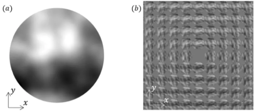
The Shack-Hartmann irradiance pattern is composed of the all microlenses irradiances and coupling between them. A generic pattern of finite extension is displayed in Fig.1(a) and highlights the periodic behavior of the wavefront sensor. Note that the irradiance pattern is split in cells in order to perform centroids extraction. In case of Fourier analysis, it is needed to take the Fourier transform of the irradiance (shown in Fig.1(b)) which is obtained by autocorrelation of the Fourier transform of the Shack-Hartmann complex amplitude (Eq. (1)). We calculate it (Fourier transform is noticed by the tilde hat):

˜A(u, v) ∝ ∏︂(︂u a, v a )︂ · Comb 1 pµL,pµL1 (u, v), (3)

with ∏︁(u/a, v/a) being a 2D door function. This one creates a frequency limit for the information, so the Fourier transform of the amplitude is made of K by K regularly spaced Dirac delta function, with K equals to:

K= 2 floor (︄ pµL2 2λ fµL )︄ + 1. (4)

Notice that the number K is always odd. The intensity recorded in the common focal plane is therefore similar to that obtained by the interference of K by K replicas of the impinging plane. This formula highlights a property of the microlens array. If one varies the focal length, pitch or wavelength, the recorded irradiance pattern still remains the same over large ranges. It corresponds to all widths of the door function which allow the selection of the same number of Dirac delta functions (Eq. (3)). Therefore, the model proposed here under monochromatic illumination is strictly valid for a significant spectral bandwidth ∆λ given by writing the wavelength interval defined for one K value of Eq. (4):

∆λ = p 2 µL f 2 K2−1. (5)

In the same logic of Ronchi [18], we propose to extend the description of the Shack-Hartmann, made here for a plan wave, to an aberrant one. Indeed, the analyzed waves are finally relatively plane and the assumption of an invariant plane wave decomposition is valid, regardless of the wave surface analyzed.

Now that the Fourier transform of the amplitude, ˜A (Eq. (3)) has been introduced, one can compute its autocorrelation to deduce the Fourier transform of the Shack-Hartmann irradiance

Fig. 1.a) The Shack-Hartmann irradiance pattern I(x, y) is presented, using a large array of

microlenses that mimic the infinite extension of the SHWFS. The microlens pitch periodicity is clearly discernable (the gold arrows and support on the inset). b) Zoom on the central part of the Fourier transform of I modulus for K = 5, which leads to get 2K − 1 = 9 harmonics in the Fourier plane, along both u and v directions. For convenience, the (0, 0) harmonic has been masked. Inverse pitch periodicity is also here visible (pink arrow).

pattern, ˜I. It is composed of 2K − 1 by 2K − 1 harmonics in both u and v directions of decreasing amplitudes. This linear decay is characteristic of the autocorrelation of the function, which is a 2D-triangle function. This description will be used as a basis for the rest of the paper; it is summarized in Fig.1(b).

Hence, we can define a generic writing for the Fourier transform of I(x, y), using ˜Hk,lwriting to define one of the (2K − 1)2_{harmonics (in Fourier space):}

˜I(u, v) ∝ K−∑︂1

k,l= −K+1

(K − |k|) · (K − |l|) · ˜Hk,l(u, v), (6)

with k and l indices allows to identify all of the harmonics. In the next section, we will inspect those harmonics.

3. Existence of multi-directional derivatives

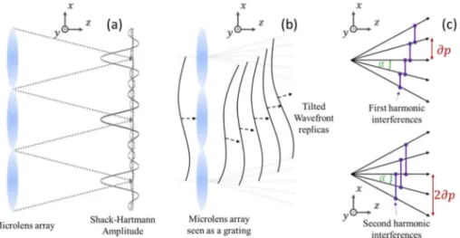
Let us now look at how the harmonics are generated in the Fourier plane, and what information do they content. The following Fig.2(a) shows the layout of the SHWFS, with a representation of its complex amplitude in the focal plane. Each point of the focal plane irradiance can be seen as the result of the interference between each of the sinc functions of the amplitude (see Eq. (1)). The irradiance will be periodic by construction of the Shack-Hartmann microlens array.

This periodicity is also to be remarked in the irradiance patterns of the lateral shearing interferometers, whose are generated by propagation of wavefront replicas created by a diffraction grating. Thus, it is possible to consider that the SHWFS irradiance pattern is generated by the propagation of the same wavefront replicas tilted by a multiple of a diffraction angle α = λ/pµL. This is equivalent to consider the microlens array as diffraction grating (Fig.2(b)) [22]. Similarly to lateral shearing interferometry, the propagation results in a shear of the wavefront replicas in the focal plane. They end up superimpose to form the complex amplitude described in Eq. (1).

Fig. 2. a) – Layout of a propagation through a SHWFS, with the complex amplitude

displayed to highlight interference effects. The gray arrows represent the focalization of the microlenses. b) – Lateral shearing-based description of the SHWFS, with the creation of multiple replicas of the impinging wavefront. Each arrow represents one of the K diffraction orders. c) – Explanation of the creation of the (1, 0) harmonic (top) and the (2, 0) harmonic (bottom). The purple lines are there to associate the interfering replicas of the propagated wavefront.

Moreover, as the Fourier transform of the amplitude (Eq. (3)) is made of K by K regularly spaced Dirac delta functions, we can finally link these functions to the K by K replicas generated by the SHWFS.

According to the SHWFS model, based on Ronchi comparison and Ref. [16], the (k, l) harmonic in the Fourier transform of the irradiance corresponds to the interferences of all wave pairs whose wave vectors are separated by kα along the x-axis and lα along the y-axis, where α is the separation angle of the microlens array seen as a lateral shearing interferometer (see Fig.2(c)). It will thus be deformed according to the local derivative in the kx + ly direction, with a shear directly proportional to the angle common to these wave pairs. At this stage of the description of the SHWFS, we can see that it measures the gradient in many directions and not only the two directions x and y considered classically.

By selecting the only harmonic (1, 0) (isolated into its 1/pµLFourier square support), re-centering it, and then performing an inverse Fourier Transform of ˜H1,0, the following expression can be derived, with the basis of [22–24] and calculus of [16,20]:

H_1,0(x, y) ∝ K−1 ∑︂ n=0 K ∑︂ m= 0 exp(i{φ[x + n∂p, y + m∂p] − φ[x + (n + 1)∂p, y + m∂p]}), (7) with the following shear:

∂p = fµL pµL

∼ pµL

K . (8)

The increment ∂p being small compared to the size of a microlens, and assuming that the phase evolves slightly and therefore linearly at the sub-pupil level, we can estimate the wavefront gradient from the expression (7) using Taylor approximation. Indeed, due to the fact that each couple of replicas generating the harmonic ˜H1,0 has the same shear ∂p (cf. Fig.2(c)), the phase difference between the n-th and the (n + 1)-th replicas remains constant, meaning that the problem is invariant along n. Therefore, for all m, n the phase difference is unchanged and can

be approximated by ∂p · ∂φ/∂x. Thus, by summation: H_1,0(x, y) = K(K − 1)exp [︃ −i ∂p ∂φ ∂x(x, y) ]︃ . (9)

Now considering the (2, 0) harmonic in Fourier space, the relevant wave pairs are shown in Fig.2(c). With the same assumption as for harmonic (1, 0), we obtain:

H_2,0(x, y) = K(K − 2)exp [︃ −i 2∂p ∂φ ∂x(x, y) ]︃ . (10)

We can see that this second harmonic measures the same x gradient as harmonic (1, 0), but with a double shear. We can also see that the amplitude of this harmonics is lower.

Finally, for the general case (k, l) harmonic inverse Fourier transform, we write: Hk,l(x, y) = (K − |k|)(K − |l|)exp [︃ −i√︁(k2+ l2)∂p ∂φ ∂xk,l(x, y) ]︃ , (11)

with xk,l, the unit vector in the direction kx + ly.

The SHWFS can therefore be described as a set of K by K mono-lateral shearing interferometers with different amplitudes, shears and shear directions. In a more general way, all the wavefront derivatives ∂φ/∂xk,lcan be deduced by this development.

4. Extraction of the derivatives

In this section, we will apply the development of sections2and3to extract the derivative of each harmonic from the Fourier plane (Fig.3(a) and3(b)). To illustrate this point, let’s consider a spherical aberration as input wavefront. This aberration, very well known by opticians has as a derivative along xk,la coma oriented in the xk,ldirection. This one is oriented and easy to recognize. We introduce a gradient matrix as a visual tool of the argument of each Hk,l (Eq. (11)),

in which hides the derivative of the wavefront along the xk,ldirection (Fig.3(c)). The shear variation√︁

(k2+ l2)∂p is discernable, increasing linearly the amplitude of the gradients.

Fig. 3.From left to right: a) Irradiance for a spherical aberration. b) Fourier Transform of

the I function. The white square delimits the extractable Fourier plane, while the yellow square represents the extraction window of the ˜H1,0harmonic. c) Matrix representation of

the comas extracted from the irradiance pattern for each harmonic of the Fourier plane. Note the orientations of the comas, all pointing towards the center of the picture. One can also note their linearly increasing amplitude.

Applying now the same process on a wave surface with more roughness than the spherical aberration, we can verify that the sensitivity of each phase derivative remains the same regardless of the harmonic chosen.

The new simulated wavefront is displayed in Fig. 4(a) and typically represents a residual optical default.

Fig. 4.a) Map of the optical default wavefront. b) Associated normalized gradients matrix,

now with shear compensation. Note that the gradients corresponding to the same orientation are almost identical.

For this Figure, compared to Fig.3, each plotted gradient was compensated by its level arm so only the term ∂φ/∂xk,lremains in the gradient matrix representation (Fig.4(b)).

As a first observation, the phase derivatives of the same orientation are almost identical, even if the new wavefront has a more roughness surface than the spherical aberration. In other words, all the harmonics of the Fourier plane preserve the same sensitivity to high variations of the wavefront and no loss of information is observed, as expected.

5. Involvement of the harmonics in the classical Fourier demodulation and the centroids extraction

We have seen, in the previous sections, that the Shack-Hartmann irradiance pattern I admits for Fourier transform a (2K − 1) · (2K − 1) harmonics array modulated by autocorrelation of the microlens individual support function ∏︁(x/pµL, y/pµL). Each of these harmonics presents a derivative of the impinging wavefront in a specific direction.

Fourier-based extraction: Classical Fourier demodulation processes, as to our knowledge, have been using only the (1, 0) and (0, 1) harmonics to compute the wavefront gradients. It is then straightforward to conclude that only the two main gradients are used to do phase retrieval.

Centroids-based extraction: We would question what information (in Fourier sense) is the Centroids extraction using, as this operation is not done in Fourier space. The complete demonstration is available to the reader in AppendixA, and we present here the main conclusions. The (p, q) centroid along x axis is typically obtained by the formula:

Cxp,q= ∫∫

Cell (p,q)x · I(x, y)dxdy ∫∫

Cell (p,q)I(x, y)dxdy

. (12)

It can also be written using Fourier derivation of the barycenter operations: Cx p,q∝ −_2iπ1 K−1 ∑︂ k=1 K − |k| k [Hk,0(p.pµL, q.pµL) − H−k,0(p.pµL, q.pµL)], (13) where we recall that Hk,0is the inverse Fourier transform of the harmonic ˜Hk,0. Unlike the classical Fourier method, the Cx _{centroids extraction only takes into account the harmonics in}

the u direction (k-summation). The same reasoning applies to the Cy _{centroids extraction and} leads to a consideration of the harmonics in the v direction only.

As a result, the centroids-based extraction is a multi-derivative process that can be seen with the Fourier formalism, however exploiting a subset of the whole information available in the Fourier plane.

To give a first indication of the potential loss related to this fact, we define here a figure of merit EX(k, l) called Excitability of harmonics which corresponds to the product of the amplitude of the harmonic with its shear.

EX(k, l) = (K − |k|)(K − |l|)√︁k2+ l2 . (14) High Excitability is suitable for performing better phase retrieval. Its representation is given in the Fig.5, with K = 5. Note that the first cross harmonics (−1, 1) and (1, 1) have values similar to those taken by the classical harmonics (1, 0) and (0, 1). More, the second and third ranks harmonics along any direction appear to have a more pronounced Excitability than the first ones. Only the harmonics very far from the center (last ring) seem to have a lower impact on the distribution of information.

Fig. 5.Excitability map of the harmonics (extractable Fourier plane) for K = 5. Note that

harmonics (2, 0) and (0, 2) seem carrying more constituent information than (1, 0) and (0, 1).

Investigating through the Excitability, we have seen that the derivatives not taken into account carry similar information than the axial ones. We now see that the weighting with the axial harmonics in the centroids extraction might be not optimal, and the same applies to the classical Fourier first harmonics demodulation. This observation paves the way for complementary studies for the development of reconstruction techniques taking into account all the harmonics and may weight them by the Excitability function, in a same logic of the work presented in the following Refs. [25,26]. By applying a similar formalism, based on a least-squares approach, and assuming a limitation by homogeneous white noise, the use of the four harmonics of the same excitability makes it possible to envisage a gain of 30% on the signal-to-noise of the reconstruction, compared to the sole use of the two classical harmonics.

6. Conclusion

The modeling presented in this paper discusses a process for the extraction of the phase derivatives along different directions of the two axes x and y. It shows that the SHWFS can be seen as a

colony of mono-lateral shearing interferometers, each related to a harmonic of the Fourier plane of the intensity recorded at the common foci of the microlenses.

Taking into account this new point of view for the SHWFS, two classical methods of phase retrieval have been revisited: the centroids extraction and the Fourier demodulation which have been correlated successfully even if their mechanism firstly seemed fundamentally different. Both methods, centroids extraction and all-harmonics Fourier formalism, highlight the redundancy of the information in the Fourier plane, which is often used for metrology purposes.

It should be noted that reconstruction on more than two derivatives, while allowing the hope of an increase in the quality of the wave surface estimate, will also result in a significant increase in processing time. This approach is rather reserved for applications that do not require real time: metrology, deconvolution from wavefront sensing [27,28]. It should also be noted that the gain in quality is all the more important as the number of harmonics is high, which corresponds to microlens matrices with the largest apertures.

The signal-to-noise gain for reconstruction will need to be further investigated for each area of SHWFS use. Indeed, the very different conditions of use between ophthalmology, astronomy, optical metrology or control of intense lasers always lead to particular limitations in terms of noise, aliasing or wrapping. Future work will focus on investigation of those different conditions, especially in regard with noise modeling.

Appendix A: demonstration of the involvement of the harmonics in the centroids extraction method

First of all, we define a Shack-Hartmann irradiance Pattern (I(x, y)) of infinite extension with the same notations as in the main corpus of the paper (see sections2and3). To calculate the (p, q) centroid in the SHWFS image, we need to apply three operations:

• Multiply by a periodic x-slope,

• Do the local average on each of the focal zone of the microlens array, • Select the central value which is the (p, q) centroid value.

Definition of the centroid operation

To define the periodic x-slope, we start defining an x-slope limited to the support of one of the microlens: r(x)= x · 1 p2_µL ∏︂(︃ x p_µL, y p_µL )︃ . (15)

This x-slope is then convoluted by a 2D Dirac comb to duplicate it onto the microlens array (we note that the function is y-invariant):

R(x, y) = r(x) ∗ CombpµL,pµL(x, y). (16)

We can write the sloped irradiance function:

I(x, y) · R(x, y) = I(x, y) · [r(x) ∗ CombpµL,pµL(x, y)]. (17)

Now, we need to average the sloped I function, this is done by convoluting the product of Iand R by a unit mean, positive, constant, weighting function, defined over the focal zone of the microlens array. It is again the support of the microlenses. To finally obtain the x-centroid

function, we need to normalize the convolution by one made with only the I function, in order to apply the same averaging process. We can write:

Cx(x′, y′)= [I(x, y) · R(x, y)] ∗ [︃ 1 p2_µL ∏︁(︂ x pµL, y pµL )︂]︃ [I(x, y)] ∗ [︃ 1 p2_µL ∏︁(︂ x pµL, y pµL )︂]︃ , (18)

with x′_{, y}′_{the variables of the convolution. It is now necessary to select the (p, q) centroid} by integrating with a delayed 2D Dirac delta function δ(x, y). This operation is again done by convolution by taking the value of the result at the (p, q) coordinates:

Cxp,q= [Cx∗δ(x − p · pµL, y − q · pµL)]. (19) This function is the classical definition of the barycenter centroid operation used in the most Shack-Hartmann applications. We want to know what Fourier information is used through these operations. So we will analyze each Fourier transform of the process.

Fourier transform analysis

The first Fourier transform (FT[.] replaces the tilde hat when the writing would be too long) is the one of the multiplication of I and R (Eq. (17)):

FT[I(x, y) · R(x, y)] = ˜I ∗ ˜R . (20) To be able to compute it, we need to calculate ˜R(u, v). We recall that the periodic x-slope function is a 2D x-sawtooth of period pµL, which admits a Fourier expansion:

R(x, y) = −1 π +∞ ∑︂ n=1 1 nsin 2πx pµL . (21)

It makes the calculation of the Fourier transform easier: ˜R(u, v) = − 1_2iπ ∑︂−1 n= −∞ 1 nδ (︃ u − n pµL, v )︃ − 1 2iπ +∞ ∑︂ n= 1 1 nδ (︃ u − n pµL, v )︃ . (22)

Now, we can fractionate the convolution in two terms (the ones of the Fourier transform of R) to facilitate the development of Eq. (20) (final frequency variables are introduced after the convolution operation to minimize the use of unnecessary letters):

˜I ∗ ˜R = − 1_2iπ [︄ −₁ ∑︂ n= −∞ 1 n˜I (︃ u − n p_µL, v )︃ +∑︂+∞ n= 1 1 n˜I (︃ u − n p_µL, v )︃]︄ . (23)

We have two separated terms that will make the rest of the demonstration easier. In term of direct space, we need now to compute the second point of the list written at the beginning of the appendix. In Fourier space, this convolution (by the microlens support anew), will be translated into a multiplication by a sinc function:

FT {︄ [I · R] ∗ [︄ 1 p2_µL ∏︂(︃ x pµL, y pµL )︃]︄ }︄ = {˜I ∗ ˜R} · 1 p2_µLsinc(pµLu) ·sinc(pµLv). (24) So, those sinc functions have an inverse pitch periodicity, which means their product is zero in each side of a square of a multiple of 1/pµLin the Fourier plane. As the SHWFS is of infinite

extension and the I irradiance pattern is pitch periodic, so those sinc functions will extinct a large number of harmonics (Eq. (24)), which we derive here for both terms:

⎧ ⎪ ⎪ ⎪ ⎪ ⎪ ⎪ ⎨ ⎪ ⎪ ⎪ ⎪ ⎪ ⎪ ⎩ −_2iπ1 −1 ∑︁ n= −∞ 1 n˜I (︂ u − _pn µL, v )︂ · 1 p2_µLsinc (︁pµLu)︁ ·sinc (︁pµLv )︁ −_2iπ1 ∞ ∑︁ n= 1 1 n˜I (︂ u −_pn µL, v )︂ · 1 p2_µLsinc (︁pµLu)︁ ·sinc (︁pµLv )︁ . (25)

All the harmonics in the v direction will be nulled due to the sinc product (period of 1/pµL). Let’s take the terms of the previous equation and we develop ˜I according to the formula of our paper (Eq. (5)): − 1 2iπ K−1 ∑︂ k= −K+1 (K − |k|) k · K · ˜Hk,0(u, v) · 1 p2_µLsinc(pµLu) ·sinc(pµLv). (26) The two terms of Eq. (25) have merged altogether. The l sum has disappeared as only the 0th term remains. Moreover, as the SHWFS is of infinite extension, the harmonics width is very thin. They only take their non-null values when n is equal to the right k.

To summarize, only the harmonics in the u-direction are saved through the averaging process. To obtain the centroid function of Eq. (18), we still need to calculate the Fourier equivalent of the quotient, which can be tedious. However, as the divider is the average irradiance over the Shack-Hartmann image, the averaged value over the support of a microlens is given by the same Dirac delta function selection process of Eq. (19). Hence, we will use it at the end of our development. It is more of a convenience, as we now know that the averaged irradiance Fourier transform has no harmonics of interest (Eq. (25) first line).

As the harmonics have a limited support, each term of Eq. (26) is only defined in the center of the Fourier plane. So the sinc product can be now omitted (i.e. = 1) to simplify the final writing of the inverse Fourier transform of the sum of the two terms in Eq. (26), to retrieve the numerator of Eq. (18): Cx(x, y) ∝ −_2iπ1 K−1 ∑︂ k=1 K − |k| k [Hk,0(x, y) − H−k,0(x, y)] , (27) Where we have reorganized Eq. (26) in order to make the inverse Fourier transform of the harmonics appear in Euler logic. Note that here, the general next step for the x-centroid extraction is to convolute with a selection by Dirac delta function for the (p, q) lens. The demonstration can be ended here, as one can see in Eq. (27), that no more v-direction nor linear combination of the Fourier harmonics, except for those on the u-direction, are involved in the information retrieval allowed by the barycenter operations (only inverse Fourier transforms Hk,0(x, y) remain in the writing).

To complete the demonstration, we are now using the knowledge of the Hk,0(x, y) value (see Eq. (11)) to simplify anew the expression:

Cx_{(x, y) ∝ +}1 π K−1 ∑︂ k=1 K − |k| k sin [︃ k∂p∂φ ∂x(x, y) ]︃ . (28)

Since the wavefront is slowly variable, we can approximate the sine, leading to: Cx_{(x, y) ∝ +}1 π∂p ∂φ ∂x(x, y) · K−1 ∑︂ k=1 (K − |k|). (29)

We now have a complete centroid function, from which we extract the value for the (p, q) microlens by convoluting with the correct Dirac delta function selector to obtain the following

equivalence:

Cx p,q∝

∂φ

∂x(p · pµL, q · pµL). (30) We recall that it is needed to normalize the result by the average value of the irradiance pattern of the Shack-Hartmann. The second one is to calibrate the SHWFS with a reference wavefront measurement, an operation which is always processed when dealing with practical applications. To conclude this appendix, we therefore conclude that the global centroids extraction only takes into account all the information of the u, v orthogonal harmonics and forsakes all other harmonics. The same reasoning applies to the y-centroid calculus.

Disclosures. The authors declare that there are no conflicts of interest related to this article. References

1. B. C. Platt and R. Shack, “History and principles of Shack-Hartmann wavefront sensing,”J. Refract Surg.17(5), S573–S577 (2001).

2. J. E. Harvey and R. B. Hooker, “Robert Shannon and Roland Shack: Legends in Applied Optics” (SPIE, 2005). 3. D. Dayton, B. Pierson, B. Spielbusch, and J. Gonglewski, “Atmospheric structure function measurements with a

Shack–Hartmann wave-front sensor,”Opt. Lett.17(24), 1737–1739 (1992).

4. L.-N. Thibos and X. Hong, “Clinical applications of the Shack-Hartmann aberrometer,”Optom Vis Sci.76(12), 817–825 (1999).

5. J. D. Mansell, J. Hennawi, E. K. Gustafson, M. M. Fejer, R. L. Byer, D. Clubley, S. Yoshida, and D. H. Reitze, “Evaluating the effect of transmissive optic thermal lensing on laser beam quality with a Shack–Hartmann wave-front sensor,”Appl. Opt.40(3), 366–374 (2001).

6. S. Le Pape, P. Zeitoun, M. Idir, P. Dhez, J. J. Rocca, and M. François, “Electromagnetic-field distribution measurements in the soft x-ray range: full characterization of a soft x-ray laser beam,”Phys. Rev. Lett.88(18), 183901 (2002). 7. M. Idir, G. Dovillaire, and P. Mercere, “Ex-and In-situ Metrology Based on the Shack-Hartmann Technique for

Sub-nanometric Metrology,”Synchrotron Radiat. News26(5), 23–29 (2013).

8. R. Irwan and R. G. Lane, “Analysis of optimal centroid estimation applied to Shack–Hartmann sensing,”Appl. Opt.

38(32), 6737–6743 (1999).

9. S. Thomas, T. Fusco, A. Tokovinin, M. Nicolle, V. Michau, and G. Rousset, “Comparison of centroid computation algorithms in a Shack–Hartmann sensor,”Mon. Not. R. Astron. Soc.371(1), 323–336 (2006).

10. D. R. Neal, J. Copland, and D. A. Neal, “Shack-Hartmann wavefront sensor precision and accuracy,” Proc. SPIE 4779, 2002.

11. N. Zon, O. Srour, and E. N. Ribak, “Hartmann-Shack analysis errors,”Opt. Express14(2), 635–643 (2006). 12. C. Canovas and E. N. Ribak, “Comparison of Hartmann analysis methods,”Appl. Opt.46(10), 1830–1835 (2007). 13. Y. Carmon and E. N. Ribak, “Phase retrieval by demodulation of a Hartmann–Shack sensor,”Opt. Commun.215(4-6),

285–288 (2003).

14. E. N. Ribak, Y. Carmon, A. Talmi, O. Glazer, O. Srour, and N. Zon, “Full wave front reconstruction in the Fourier domain,”Proc. SPIE6272, 627254 (2006).

15. Y. Mejía, “Noise reduction in the Fourier spectrum of Hartmann patterns for phase demodulation,”Opt. Commun.

281(5), 1047–1055 (2008).

16. J. Primot, “Theoretical description of Shack–Hartmann wave-front sensor,”Opt. Commun.222(1-6), 81–92 (2003). 17. F. Hénault and C. Pannetier, “Hartmann vs reverse Hartmann test: a Fourier optics point of view,” Proc. SPIE 11102,

111020C (2019).

18. V. Ronchi, “Forty years of history of a grating interferometer,”Appl. Opt.3(4), 437–451 (1964).

19. M. Lombardo and G. Lombardo, “New methods and techniques for sensing the wave aberrations of human eyes,” Aust. J. Optom.92(3), 176–186 (2009).

20. Y. Dai, F. Li, X. Cheng, Z. Jiang, and S. Gong, “Analysis on Shack–Hartmann wave-front sensor with fourier optics,” Opt. Laser Technol.39(7), 1374–1379 (2007).

21. M. A. Betanzos-Torres, J. Castillo-Mixcóatl, S. Muñoz-Aguirre, and G. Beltrán-Pérez, “Adaptive optics system simulator,”Opt. Laser Technol.105, 118–128 (2018).

22. F. Roddier, “Variations on a Hartmann theme,” Opt. Eng. 29(10) (1990).

23. M. Takeda, H. Ina, and S. Kobayashi, “Fourier-transform method of fringe-pattern analysis for computer-based topography and interferometry,”J. Opt. Soc. Am.72(1), 156–160 (1982).

24. C. Roddier and F. Roddier, “Interferogram analysis using Fourier transform techniques,”Appl. Opt.26(9), 1668–1673 (1987).

25. R. Legarda-Sáenz, M. Rivera, R. Rodríguez-Vera, and G. Trujillo-Schiaffino, “Robust wave-front estimation from multiple directional derivatives,”Opt. Lett.25(15), 1089–1091 (2000).

26. S. Velghe, J. Primot, N. Guérineau, M. Cohen, and B. Wattellier, “Wave-front reconstruction from multidirectional phase derivatives generated by multilateral shearing interferometers,”Opt. Lett.30(3), 245–247 (2005).

27. J. Primot, G. Rousset, and J.-C. Fontanella, “Deconvolution from wave-front sensing: a new technique for compensating turbulence-degraded images,”J. Opt. Soc. Am. A7(9), 1598–1608 (1990).

28. J. A. Koch, R. W. Presta, R. A. Sacks, R. A. Zacharias, E. S. Bliss, M. J. Dailey, M. Feldman, A. A. Grey, F. R. Holdener, J. T. Salmon, L. G. Seppala, J. S. Toeppen, L. Van Atta, B. M. Van Wonterghem, W. T. Whistler, S. E. Winters, and B. W. Woods, “Experimental comparison of a Shack–Hartmann sensor and a phase-shifting interferometer for large-optics metrology applications,”Appl. Opt.39(25), 4540–4546 (2000).