HAL Id: hal-03189295
https://hal-amu.archives-ouvertes.fr/hal-03189295
Submitted on 3 Apr 2021
HAL is a multi-disciplinary open access
archive for the deposit and dissemination of
sci-entific research documents, whether they are
pub-lished or not. The documents may come from
teaching and research institutions in France or
abroad, or from public or private research centers.
L’archive ouverte pluridisciplinaire HAL, est
destinée au dépôt et à la diffusion de documents
scientifiques de niveau recherche, publiés ou non,
émanant des établissements d’enseignement et de
recherche français ou étrangers, des laboratoires
publics ou privés.
Parametric measurements and analysis with MPAS
model
M Chiletti, J Duchateau, F Topin, B Turck, L Zani
To cite this version:
M Chiletti, J Duchateau, F Topin, B Turck, L Zani. Void fraction influence on CICCs coupling
losses: Parametric measurements and analysis with MPAS model. IEEE Transactions on Applied
Superconductivity, Institute of Electrical and Electronics Engineers, 2020. �hal-03189295�
Void fraction influence on CICCs coupling losses:
Parametric measurements and analysis with MPAS model
M. Chiletti, J.L. Duchateau, F. Topin, B. Turck, and L. Zani.
Abstract— Modelling by analytical approach the coupling losses
of CICCs used in tokamaks remains a challenge to be reliable. This is usually done using either CPU consuming numerical approaches or heuristic models such as MPAS now used for ITER. Experimental measurements of AC losses are performed at CEA using magnetization method on several JT-60SA TF type samples with various void fractions (25%-36%). Influence of void fraction on coupling losses is hard to heuristically model yet. We choose to develop an experimental protocol in order to measure coupling losses in a range of frequency relevant to fusion operation domain. AC losses model as MPAS is confronted to our JOSEFA experimental data. Conclusion and lessons will be taken into account for future work.
Index Terms— nuclear fusion, AC losses, superconducting
magnets, CICCs, void fraction.
I. INTRODUCTION
Experimental measurements of AC losses in the fusion community are mainly performed in SULTAN facility [1] [2] [3] [4]. All measurement performed on various geometry of CICC confers to the community a wide catalogue of the influence of parameters on coupling losses. These variations of parameters (void fraction, twist pitches, etc.) on a same cable is hard to set up either for technical reason (production, reproducibility) or for financial reason (cost). Using JOSEFA facility at CEA Cadarache, we perform AC losses measurements on several conductor samples of JT-60SA TF type (labelled MAG42-1 to 6) that were produced for hydraulic tests purposes [5] and show various void fractions, ranging from 25% to 36% and on a sample extracted from (DP4-UP corresponding to MAG42-3 in terms of geometry and void fraction). The influence of the void fraction parameter on the coupling losses can therefore be quantified and verified without risk of other parameters influence (strand type, twist pitch, cabling procedure, etc.) [6]. AC losses are generated by sinusoidal applied field (named 𝐵𝑎𝑝𝑝) in order to constitute an experimental database easy to directly confront with those led e.g. at SULTAN facility. On the other hand for exemple, the influence of the void fraction can also be investigated to get insights on the conductances to be used in COLISEUM [7]. Increase of the void fraction could be related to an increase in the inter stages transverse conductances. Model as MPAS [8] is confronted to these experimental measurements in order to give us a better description of AC losses (contribution of each stage) than the one time constant approach.
Manuscript submitted for review Sept 24, 2019. This work was supported in part by ASSYSTEM.
M. Chiletti (corresponding author phone: +33442254749; e-mail:
[email protected]), L. Zani, B. Turck and JL. Duchateau are with Commissariat à l’Energie Atomique et aux Energies Alternatives, CEA/DRF/IRFM, CEA Cadarache 13108 St Paul-Lez-Durance, France. M.Chiletti is also with Aix Marseille Université, CNRS, IUSTI UMR 7343, 13453, Marseille, France together with F. Topin.
II. EXPERIMENTAL FACILITY :JOSEFA
JOSEFA facility [9] is used to measured AC losses generated in large superconducting cables. The method is described below. Our superconducting samples are 𝐿 = 300 𝑚𝑚 long (JT-60SA TF last stage twist pitch) with an approximate cable cross section of 18 × 22 𝑚𝑚 depending on the compaction rate [10]. As the applied field is transverse to the larger side of the sample, pick-ups are wound longitudinally on the CICC (Cable In Conduit Conductor) and on an epoxy replica with same dimensions. Tests are conducted in a Helium bath at 4,2 𝐾. A superconducting dipole is used to generate the transverse magnetic field, uniform on the whole length of the CICC sample. We scan sinusoidal field frequencies ranging from 5 𝑚𝐻𝑧 (to get refined data for ntau determination) up to 4 𝐻𝑧 (to deeply investigate ranges where single constant model likely becomes invalid). Our power supply having operating limitations, amplitude of the input current decrease with frequency but in a reasonable range which does not affect the coupling losses while rescaling with 𝐵𝑖2[11]. 𝐵𝑖 being the internal field of the CICC in response to the applied external field.
The wound coils tensions generated by pulsed field are balanced with a Wheatstone bridge to isolate a tension 𝑉𝑚 produced by the magnetization of the sample. That magnetization 𝑀 is directly related to the total losses 𝑄 generated by the CICC.
𝑄 = ∫ 𝑀𝑑𝐵𝑎𝑝𝑝= −𝑓𝑔𝑒𝑜∫ (∫ 𝑉𝑚𝑑𝑡) 𝑑𝐵𝑎𝑝𝑝
with 𝑓𝑔𝑒𝑜 being the geometrical factor correction for these square samples. This geometrical factor is computed using analytical tools from [12]: 𝑓𝑔𝑒𝑜= 4𝑦𝑖 𝜇0𝑅𝑏𝑟𝑖𝑛2 𝑛𝑠𝐿𝑛𝑐(2 atan (𝑦𝑥𝑖 𝑖) − atan ( 𝑦𝑖+ 𝑦𝑒 𝑥𝑖 ) − atan ( 𝑦𝑖− 𝑦𝑒 𝑥𝑖 ))
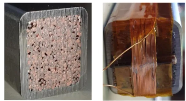
and verified using tomographic slices [13] plus step induced current simulation of our cables. 𝑛𝑠 and 𝑛𝑐 are respectively the strand number and the pick-up coil turn number. 𝑥 and 𝑦 are coordinate of the pick-up position in our experiment referential. Vid fraction of the six tested samples are gathered in table I and a picture of a sample is shown in Fig. 1.
Fig. 1. MAG42-2, cross section of tested samples. 486 strands of 0.81 mm of diameter, with 324 of superconducting strands. Without (left) and with (right) the wound measurement pick-up coil.
Table I Void Fraction of Samples.
MAG42 1 2 3 (DP4) 4 5 6
Void Fraction
(%) 35.6 33.2 31.6 31.5 30.2 28.1 25.9
Two components contribute to the total losses, the hysteresis losses 𝑄ℎ and the coupling losses 𝑄𝑐 .
III. HYSTERESIS LOSSES
The description of 𝑄ℎ will differ if the applied field 𝐵𝑎𝑝𝑝= 𝐵𝑚sin(𝜔𝑡) + 𝐵𝑜𝑓𝑓 is above or below the penetration field 𝐵𝑝 :
𝐵𝑝𝑡ℎ𝑒𝑜 =
2𝜇0𝑑𝑒𝑓𝑓𝐽𝑐∗(𝐵𝑖) 𝜋
where 𝑑𝑒𝑓𝑓 is the strand effective superconducting filament diameter, and 𝐽𝑐∗(𝐵𝑖) is the critical current density of the strand integrated over the internal field variation:
𝐽𝑐∗(𝐵𝑖) = 𝐽𝑐(𝐵𝑜𝑓𝑓) + ∫ 𝐽𝑐 𝑑𝐵 𝐵𝑜𝑓𝑓+𝐵𝑖
𝐵𝑜𝑓𝑓−𝐵𝑖 .
The value of 𝐽𝑐∗ is accurately calculated using past experimental measurement on the K006-01C strand using VSM technique [1]. 𝐵𝑝 is the field limit above which currents penetrate until the center of the superconducting filaments. In the following work we will principally use the partial penetration approach in which 𝛽 = 𝐵𝑖
𝐵𝑝𝑡ℎ𝑒𝑜≤ 1. On the other side, 𝑑𝑒𝑓𝑓 is initially taken at its nominal value: 18 𝜇𝑚, as defined by the manufacturer. In this case, the expression of hysteresis losses can be written:
𝑄ℎ𝑦𝑠𝑡= 2𝜋𝐵𝑖3 6𝜇02𝐽 𝑐∗(𝐵𝑖)𝑑𝑒𝑓𝑓(1 + 𝑥) (1 − 𝜋𝐵𝑖 4𝜇0𝐽𝑐∗(𝐵𝑖)𝑑𝑒𝑓𝑓 ) (1) in the few cases where 𝛽 > 1 the previous expression rewrites
𝑄ℎ𝑦𝑠𝑡= 4𝐽𝑐∗(𝐵𝑖)𝑑𝑒𝑓𝑓𝐵𝑖 3𝜋(1 + 𝑥) (13 − 𝜇0𝐽𝑐∗(𝐵𝑖)𝑑𝑒𝑓𝑓 𝜋𝐵𝑖 ) (2) both expressed in 𝐽. 𝑚−3. 𝑐𝑦𝑐𝑙𝑒−1 of composite strand with 𝑥 being the ratio of non-superconducting material over superconducting ones (𝑥 = 1.94 in JT-60SA CICC). Formulae elaborated by B.Turck gathered in [14]. It is referred to the surface of composite inside the CICC. The above formulae (1) and (2) agree with the two developed by M.Wilson [15] (with less than 5 % discrepancy) and will be used to discriminate hysteresis losses and coupling losses within the experimental data. We can also note that 𝐵𝑝𝑡ℎ𝑒𝑜= 0.169 𝑇.
Indication on the effective filament diameter 𝑑𝑒𝑓𝑓 will be given after a statistical study of the measured hysteresis losses data.
Fig. 2. Magnetization cycle with major hysteresis losses generated, at f=0.005 Hz with 𝐵𝑚= 0.2 𝑇 and 𝐵𝑜𝑓𝑓= 0.5 𝑇.
Firstly, we can see that the 𝐵𝑝𝑡ℎ𝑒𝑜≈ 𝐵𝑝𝑒𝑥𝑝 (within 2.4%). As
coupling losses are generated under field variation, when 𝑓 = 0 𝐻𝑧, only hysteresis losses remain. Thus, the ordinate at origin of total losses data curves provides us the experimental hysteresis losses. These hysteresis losses correspond nearly to the area of a cycle for 𝑓 → 0 as depicted below in Fig. 2. Area of the cycle in Fig. 2 (for 𝑓 = 5 𝑚𝐻𝑧) contains few coupling losses as the zoom in Fig. 3 confirms (around 1.5 𝑚𝐽. 𝑐𝑚−3. 𝑐𝑦𝑐𝑙𝑒−1). Measured 𝑄ℎ𝑒𝑥𝑝 are extracted using linear regressions in the 0.5 − 0.15 𝑚𝐻𝑧 range. They can be perfectly fitted adjusting the effective filament diameter of formulae (1) and (2). Using these methods on all our samples tests ( ~20 𝑄(𝑓) curves of 35 points each) allow us to gather a statistic of 20 value of 𝑑𝑒𝑓𝑓 which over all samples gives us a statistical value of 17,6 ± 1,0 𝜇𝑚. We can notice that this statistical study has been led for varying 𝐵𝑜𝑓𝑓, 𝐵𝑚 and void fractions and nevertheless was in very good agreement (within 2%) with the manufacturer data, consolidating our method. Our hysteresis losses modelling being reliable we can consider coupling losses from our post processing are robust.
IV. COUPLING LOSSES COMPARISON WITH SULTAN Coupling losses are generated by coupling current looping through resistive zone of the cable (copper, CuNi, etc.) and appears only when field varies.
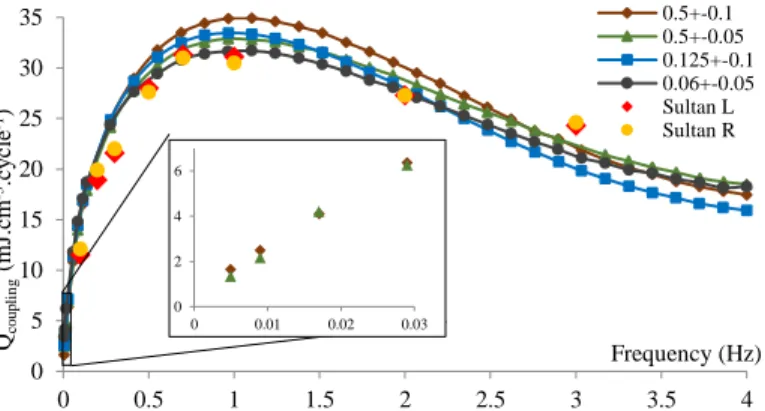
Fig. 3. Coupling losses on MAG42-3, similar to JT-60SA TF production cable. JOSEFA data comparison with SULTAN left and right leg. All curves are rescaled to 𝐵𝑚= 0,1𝑇, the amplitude of SULTAN measurements. Included curves zoom in to confirm the good extrapolation.
As we can see in the above Fig.
3
, our measurement using magnetization method agree very well with the calorimetric measurement led at SULTAN facility [1] in terms of slope at origin and position of the maximum of the curves. This consolidates our experimental process of AC losses measurement and our post processing, especially the rescaling with 𝐵𝑖2 of the different measurements done on each samples. However at 3 Hz some discrepancy seems to appear (within 14%). This discrepancy could be generated by the difference in our measurement and post processing methods: calorimetric for SULTAN and magnetization for JOSEFA. Post processing methods are also different and helium mass flow could have been badly interpreted in calorimetric measurement. We can also take into account the fact that our sample is 30 cm long while in SULTAN the length of the leg is about 2 meter. Considerations on the conductor length influence on AC losses (see Ries and Takacs in [16]) showed that such punctual differences could appear. We consider consequently that our results on JOSEFA are trustworthy to be for further study.0 5 10 15 20 25 30 35 0 0.5 1 1.5 2 2.5 3 3.5 4 Qco u p li n g (mJ.c m -3.c y cl e -1) Frequency (Hz) 0.5+-0.1 0.5+-0.05 0.125+-0.1 0.06+-0.05 Sultan L Sultan R 0 2 4 6 0 0.01 0.02 0.03 𝐵𝑝𝑒𝑥𝑝= 0.165 𝑇 𝐹𝑢𝑙𝑙𝑦 𝑝𝑒𝑛𝑒𝑡𝑟𝑎𝑡𝑒𝑑
We can also notice on a same sample that our different measurements changing either 𝐵𝑜𝑓𝑓 or Δ𝐵 are well agreed with each other when rescale to the same Δ𝐵. From the 𝑄(𝑓) slope at origin, we can extract the effective 𝑛𝜏, written 𝑛𝜏𝑒𝑓𝑓, of the cable in order to apply the single time constant model where 𝑃 = 𝑛𝜏𝑒𝑓𝑓𝐵̇𝑖2
𝜇0 . Applying this method on our 6 samples, we obtain the
variation of 𝑛𝜏𝑒𝑓𝑓 with respect to the void fraction of samples.
Fig. 4. Variation of 𝑛𝜏𝑒𝑓𝑓 with respect to the CICC void fraction. Error bars are standard deviation over each sample 𝑛𝜏𝑒𝑓𝑓 statistic.
DP4-UP and MAG42-3 very close to each other as their geometrical parameters are almost identical, except that DP4 is strictly part of the JT-60SA TF coil production whereas the MAG42-3 was manufactured separately. This consistency comforts us in our global methodology. Compacting the cable to go from 36% to 26% void fraction multiply the 𝑛𝜏𝑒𝑓𝑓 with a factor 3. As suspected, 𝑛𝜏𝑒𝑓𝑓 is increasing with the decreasing void fraction. This is related to the trustworthy hypothesis that interstages conductances increase with compaction rate [17], as a consequence of inter-strand surface growth. This hypothesis has already been confirmed using theoretical model as COLISEUM [7] where time constant and transverse conductances (𝜎′𝑠) are linearly related with homothetic transformation of 𝜎′𝑠. In order to obtain comparable 𝑛𝜏𝑒𝑓𝑓 with COLISEUM, 𝜎′𝑠 ranges are around 108 𝑆. 𝑚−1, confirmed with evaluation from Twente University [18]. This item is currently under further investigation using tomographic images of the samples and should be subject of a future publication.
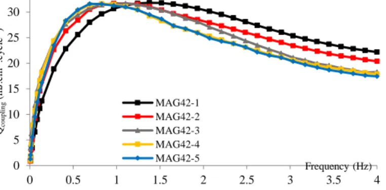
Apart from increasing the 𝑛𝜏𝑒𝑓𝑓, we can notice that increasing the compaction of MAG42 samples does modify the frequency where 𝑄(𝑓) curve reach its maximum (see Fig. 5 and reported in the TABLE below). Amplitudes and global curves shape is conserved with void fraction variation.
Fig. 5. Comparison of 𝑄(𝑓) curves for various void fractions for 𝐵𝑚= ±0.1 𝑇.
TABLE II
Position of the maximum of the 𝑄(𝑓) curves for MAG42 and DP4 samples.
MAG42- 1 2 3 DP4 4 5
Max. pos.
(Hz) 1.38 1.23 1.1 1.08 0.86 0.82
*MAG42-6 is not reported here due to the absence of data above 0.5 Hz.
This modification of 𝑛𝜏𝑒𝑓𝑓 and of the maximum position could be related with the redistribution of inter-stage conductances, modifying the contribution of each stage to the global losses. As six samples of 30 cm are compacted to different void fraction (MAG42), interstages effective conductances distribution can be different regarding the sample. At the end, data post processing is well established, results are consistent with previous tests (TFCS2 in SULTAN) and with each other’s (different series). MPAS will try to give us a description of the contribution of each stage to these measured data.
V. CONFRONTATION WITH MPAS
We can see in Fig. 6 that checking the single time constant model (usually applied in the fusion community) to our experimental data adjusting the 𝑛𝜏𝑒𝑓𝑓 shows overestimates coupling losses at low frequency (0.05-0.6 Hz) and then highly underestimates them on the rest of the range (at least 40% from 2Hz on). Same behaviour is observed, even more pronounced for some, with other MAG42 sample.
Fig. 6. Single time constant model versus experimental data issued from measurement on MAG42-3 for 𝐵𝑚= 0.1𝑇.
It confirms the necessity to use a more elaborated model to describe the coupling losses generated in a CICC. For this reason, we consider the model MPAS formerly developed at CEA [8] and confront it with the experimental data. In its initial development MPAS fits the whole coupling losses curve with a minimum degrees of freedom adjusting only the last stage features (time constant 𝜏 and shielding coefficient 𝑛𝜅). Then, geometrical constraints between the different stages (issued from cable physics) analytically couple the 𝜏 and 𝑛𝜅 from sub-stages to the ones of the last stage.
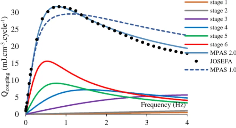
Recent MPAS enhancement includes the strand contribution in the coupling losses description and allows the last stage to be decoupled from sub-stages ones. This is due to the fact that last stage is a sextuplet, so the relation between the fourth and last stage are not driven the same way than the other stages are. It is thus the shielding coefficient and the time constant of the fourth stage that drives the other ones. We can see in the figure below (Fig. 7) the comparison between the original MPAS and the enhanced MPAS regarding the coupling losses issued from JOSEFA facility. Decoupled COLISEUM [7] gives us the relation between decoupled 𝜏 to tell that time constant of fifth
0 200 400 600 800 1000 0.25 0.27 0.29 0.31 0.33 0.35 n teff (ms) Void Fraction 0 5 10 15 20 25 30 0 0.5 1 1.5 2 2.5 3 3.5 4 Qco u p li n g (m J. cm -3.c y c le -1) Frequency (Hz) MAG42-1 MAG42-2 MAG42-3 MAG42-4 MAG42-5 0 5 10 15 20 25 30 35 0 0.5 1 1.5 2 2.5 3 3.5 4 Qco u p li n g (mJ.c m -3.c y cl e -1) Frequency (Hz) One time constant
and fourth stage are closer than the usual twist pitch ratio when going from a triplet to a sextuplet. This assertion gives us an interval to adjust our last stage time constant:
𝜏4= 𝜏5 [ 𝜎4𝛾4sin2(𝑁𝜋 4) 𝑙𝑝4 2 𝜎5𝛾5sin2( 𝜋 𝑁5) 𝑙𝑝5 2 ; ( 𝑙𝑝4 𝑙𝑝5 ) 2 ] (3). This confrontation shows the limit of the constraint applied to the original MPAS in fact, both low and high frequency cannot be fitted using the classical MPAS constraints (squared twist pitch ratio)
.
Fig. 7. Confrontation of both MPAS 1.0 (dashed) and MPAS 2.0 (plain) with experimental data from SULTAN and JOSEFA on MAG42-3.
In fact, last stage (5th) is decoupled from the four others and does
not affect their behaviour anymore but guided by the new constraint rule (3). Doing this splitting inside MPAS, allow us to fit both high and low frequency at the same time with a better agreement (Fig. 7) than with the fully coupled MPAS.
TABLE III
Time constants (bold) and shielding coefficients (normal) repartition using the model MPAS 1.0 and the MPAS 2.0 on MAG42-3 sample and SULTAN.
VI. DISCUSSION
We can see that new MPAS version can model the behaviour at low and high frequency of the experimental data giving approximately the same 𝑛𝜏𝑒𝑓𝑓 for JOSEFA and SULTAN. With a closer look, we can see that time constants and shielding coefficients (ponderation of each stage contribution) repartition among stages are slightly different regarding the chosen approach.
𝑛𝜏
𝑒𝑓𝑓(Table III)
are in good agreement but stagescontribution (𝑛𝜅) are slightly different for the three last stages that could be explained by the difference in the distribution of inter-stage conductances as explained before. Last stage contribution is more weighted in MAG42-3 sample than in TFCS2 one. We can also notice that other substage shielding
coefficient repartition is different in MAG sample than in SULTAN sample.
The results of measurements performed on the MAG42 samples are two-folded: first they confirm the experimental measurement led at SULTAN on the JT-60SA TF, and they give us the information needed concerning conductances ranges we have to put into COLISEUM to well fit the data without any electrical measurement of resistance using the CICC. On the other side we could reverse the process and use electrical measurement of inter stage conductances to predict coupling losses without any AC losses measurement.
Peculiar behavior noticed in Fig. 5 has already been observed in the two stage model only [7] modifying the set of conductances.
VII. CONCLUSION
In this complete study, we have used magnetization method to measure the total losses generated by CICC samples. Our hysteresis losses removal gives us a statistic on the effective diameter of the superconducting NbTi filaments in our samples. The manufacturer value for this diameter agrees well with the experimental filament diameter found. Globally, experimental methods viability is confirmed and allows us to perform a complete study of AC losses in superconducting samples. The variation of 𝑛𝜏𝑒𝑓𝑓 with void fraction is quantified, it can be related to the increasing compaction of the cable and thus to the increasing interstages effective transverses conductances. Amplitude of 𝑄𝑐𝑜𝑢𝑝𝑙𝑖𝑛𝑔 curves is conserved while the maximum of losses is moving toward low frequency while increasing the compaction of the cable. Coupling losses measurements are of good quality and well agree with each other when rescale to the same 𝐵𝑚 . This gives us a big statistical database for study. Unique time constant approach is inefficient to accurately describe the coupling losses generated by a CICC so we firstly use the original MPAS model developed at CEA. This does not give us an accurate description of the measured losses, we have to change the coupling rules of the last stage in order to give it more weight in the fit. Thus the MPAS 2.0 used in this paper contains the five stages contributions plus the strand one and well agree with experimental data.
Further enhancement will be led on MPAS using the recent implementation of COLISEUM to an N stage model, for example precise the new constraint rule to bond the fifth and fourth stage. At the end, the magnetic behavior of the CICC modelled using COLISEUM will help us unconstraint the MPAS model.
Also, new measurements and post processing might be led in JOSEFA facility using other CICC sample for example TFJS1 [18] or ITER correction coil for their full superconducting wiring. CEA models will be confronted to this new database to benchmark and confirm their robustness in their new version.
ACKNOWLEDGMENTS
I would like to thank M. Tena, D. Arranger, G. Jiolat, J. Llorens and D. Guibert for their technical support during the whole experimental campaign of AC losses measurement using JOSEFA facility at CEA Cadarache.
We also thank ASSYSTEM and S.Constant for their financial support during this work and the whole PhD.
0 5 10 15 20 25 30 0 1 2 3 4 Qco upl in g (m J.c m -3.c y cle -1) Frequency (Hz) stage 1 stage 2 stage 3 stage 4 stage 5 stage 6 MPAS 2.0 JOSEFA MPAS 1.0 MPAS 1.0 MAG42-3 MPAS 2.0 MAG42-3 MPAS 2.0 TFCS2 Stage n° 𝑛𝜅 𝜏 (𝑚𝑠) 𝑛𝜅 𝜏 (𝑚𝑠) 𝑛𝜅 𝜏 (𝑚𝑠) 0 (strand) 0.1 7 0.29 18.4 0.3 18.4 1 0.36 4.5 0.39 4.8 2 0.54 21.5 0.46 35.6 0.51 37.3 3 0.66 63.3 0.58 105 0.67 110 4 0.89 127 0.73 210 0.87 220 5 1.2 370 1.25 300 1.0 330 Overall (Σ𝑛𝜅𝜏) (ms) 613 611 621
REFERENCES
[1] L. Zani et al., "Experimental and Analytical Approaches on JT—60SA TF Strand and TF Conductor Quality Control During Qualification and Production Manufacture Stages" in IEEE Transactions on Applied Superconductivity, vol. 23, no. 3, pp. 4200504-4200504, June 2013, Art no.4200504.DOI: 10.1109/TASC.2012.2232951.
[2] Nijhuis, A., Ilyin, Y., & Abbas, W. (2006). “ Effect of void fraction and petal wraps on the AC loss, Rc and mechanical properties of ITER conductors.” Enschede: Final Report Contract No. EFDA-04/1136, UT-EFDA 2006-1.
[3] Breschi, Marco & Bianchi, Marco & Ricchiuto, Anna & Ribani, P.L. & Devred, Arnaud. (2017). “Analysis of AC losses in a CS conductor sample for the ITER Project”. IEEE Transactions on Applied Superconductivity. PP. 1-1. 10.1109/TASC.2017.2785404.
[4] D. Bessette, "Design of a Nb3Sn Cable-in-Conduit Conductor to Withstand the 60 000 Electromagnetic Cycles of the ITER Central Solenoid," in IEEE Transactions on Applied Superconductivity, vol. 24, no. 3, pp. 1-5, June 2014, Art no. 4200505. doi: 10.1109/TASC.2013.2282399.
[5] L. Zani, F. Bonne, D. Ciazynski, P. Decool, G. Gros, C. Hoa, P. Hertout, B. Lacroix, V. Lamaison, Q. Le Coz, N. Misiara, S. Nicollet, F. Nunio, J.-M. Poncet, R. Radhakrishnan, A. Torre and R. Vallcorba, “Progresses at CEA on EU demo reactor cryomagnetic system design activities and associated R&D”, Nuclear Fusion, Vol. 59 Art. 086033 (2019).
[6] Nijhuis, Arend & Kate, Herman & Bruzzone, Pierluigi & Bottura, Luca. (1996). “Parametric Study on Coupling Loss in Subsize ITER Nb3Sn Cabled Specimen.” Magnetics, IEEE Transactions on. 32. 2743 - 2746. 10.1109/20.511442.
[7] M. Chiletti, J. Duchateau, F. Topin, B. Turck and L. Zani, "Analytical Modelling of CICCs Coupling Losses: Broad Investigation of Two-Stage Model," in IEEE Transactions on Applied Superconductivity, vol. 29, no. 5, pp. 1-5, Aug. 2019, Art no. 4703005. DOI: 10.1109/TASC.2019.2907779. [8] B. Turck, L. Zani, “A macroscopic model for coupling current losses in
cables made of multistage of superconducting strands and its experimental validation.”, Cryogenics, Volume 50, Issue 8, 2010, Pages 443-449, ISSN 0011-2275.
[9] P. Decool et al., "The CEA JOSEFA test facility for subsize conductors and joints," in IEEE Transactions on Applied Superconductivity, vol. 14, no. 2, pp.1473-1476, June 2004. doi: 10.1109/TASC.2004.830657
[10] L. Zani, P. Barabaschi, M. Peyrot, “Starting EU production of strand and conductor for JT-60SA Toroidal Field coils”, IEEE Transactions on Applied Superconductivity Vol. 22 n°3, p.4801804 (2012).
[11] J. L. Duchateau, B. Turck, B. Lacroix, M. Schwarz, A. Torre and L. Zani, "Stability of a cable in conduit conductor under fast magnetic field variations," in IEEE Transactions on Applied Superconductivity, vol. 22, no. 3, pp. 4803205-4803205, June 2012, Art no. 4803205. DOI: 10.1109/TASC.2011.2181140.
[12] T.Schild. « Mesures de pertes par aimantation : Principe et Méthode d’analyse » CEA Internal Service Technical Note NT/EM/98/33.
[13] Ion Tiseanu, Louis Zani, Teddy Craciunescu, Florin Cotorobai, Cosmin Dobrea, Adrian Sima, “Characterization of superconducting wires and cables by X-ray micro-tomography”, Fusion Engineering and Design, Volume 88, Issues 9–10, 2013, Pages 1613-1618, ISSN 0920-3796, https://doi.org/10.1016/j.fusengdes.2013.03.065.
[14] B.Turck. CEA Internal Service Note TS41, Feb. 1985.
[15] M.N. Wilson, “Time-varying fields and AC losses”, Superconducting Magnets, Oxford, Oxford University Press, p.166-169.
[16] G. Ries and S. Takacs, "Coupling losses in finite length of superconducting cables and in long cables partially in magnetic field," in IEEE Transactions on Magnetics, vol. 17, no. 5, pp. 2281-2284, September 1981.DOI: 10.1109/TMAG.1981.1061354.
[17] Nijhuis, Arend & Ilyin, Yu & Abbas, Wasan & Kate, Herman & Ricci, M.V. & Corte, A.. (2005). “Impact of Void Fraction on Mechanical Properties and Evolution of Coupling Loss in ITER Nb3Sn Conductors under Cyclic Loading. Applied Superconductivity”, IEEE Transactions on. 15. 1633 - 1636. 10.1109/TASC.2005.849214.
[18] A. Nijhuis, Yu. Ilyin, W. Abbas, B. ten Haken, H.H.J. ten Kate, “Change of interstrand contact resistance and coupling loss in various prototype ITER NbTi conductors with transverse loading in the Twente Cryogenic Cable Press up to 40,000 cycles”, Cryogenics, Volume 44, Issue 5, 2004, Pages
319-339, ISSN 0011-2275,
https://doi.org/10.1016/j.cryogenics.2004.01.001.
[19] Zani, Louis et al. “Tests and Analyses of Two TF Conductor Prototypes for JT-60SA.” IEEE Transactions on Applied Superconductivity 20 (2010): 451-454.