Modèles de régression à inflation de zéro et données
censurées - application au recours aux soins de santé
Zero-inflated regression models for right-censored counts, with an
application to healthcare utilization
Van Trinh Nguyen1, Jean-François Dupuy2
1Univ Rennes, INSA Rennes, CNRS, IRMAR - UMR 6625, F-35000 Rennes, France, Van-Trinh.Nguyen@insa-rennes.fr 2Univ Rennes, INSA Rennes, CNRS, IRMAR - UMR 6625, F-35000 Rennes, France, Jean-Francois.Dupuy@insa-rennes.fr
RÉSUMÉ. Les modèles de régression à inflation de zéro ont été peu étudiés dans le cas où la variable réponse est censurée. Dans cet article, nous nous intéressons aux propriétés de l’estimateur du maximum de vraisemblance dans les modèles de régression à inflation de zéro de Poisson et négatif binomial, lorsque le comptage d’intérêt est censuré à droite. Ces propriétés sont évaluées au moyen de simulations. Nous discutons également la question de la sélection de variables dans ces modèles. Enfin, nous décrivons une application à un jeu de données relatif à la consommation de soins de santé.
ABSTRACT. Zero-inflated models for censored and overdispersed count data have received little attention so far, except for the zero-inflated Poisson (ZIP) model which assumes that overdispersion is entirely caused by zero-inflation. When additional overdispersion is present, useful alternatives to ZIP are given by the zero-inflated generalized Poisson (ZIGP) and zero-inflated negative binomial (ZINB) models. This paper investigates properties of the maximum likelihood estimator (MLE) in ZIGP and ZINB regression models when the count response is subject to right-censoring. Simulations are used to examine performance (bias, mean square error, coverage probabilities and standard error calculations) of the MLE. Results suggest that maximum likelihood yields accurate inference. A simple, efficient and easy-to-implement methodology for variable selection is also proposed. It is applicable even when the number of predictors is very large and yields interpretable and sound results. The proposed methods are applied to a dataset of healthcare demand.
MOTS-CLÉS. Excès de zéros, maximum de vraisemblance, simulations.
KEYWORDS. Excess of zeros, maximum likelihood, simulations.
1. Introduction
Healthcare utilization refers to the measure of a population’s use of available healthcare services. It is often reported as the number of healthcare services (e.g., hospital resources, physician resources) used over a period of time. Count-valued outcomes arising from healthcare utilization studies can be modeled using discrete distributions, such as Poisson or negative binomial. However, healthcare uti-lization data often contain large numbers of zeros, i.e. there is a large number of non-users of the corresponding healthcare service over the study period. When there are more zeros than expected un-der a standard count model, the data are said to be inflated, which is a particular cause of zero-inflation.
Various models have been developed to address zero-inflation, such as zero-inflated (ZI) models which mix a degenerate distribution at zero with a standard count model. If predictors are present (e.g., age, in-come, health satisfaction), ZI models can be extended to the regression setting by modeling zero-inflation and count sub-distributions as functions of the predictors. For example, zero-inflated Poisson (ZIP) re-gression model was proposed by LAMBERT (1992), and further developed to accommodate random effects (HALL, 2000 ; MIN AND AGRESTI, 2005 ; MONOD, 2014), non-linear covariate effects (LAM ET AL., 2006 ; HE ET AL., 2010 ; LU AND LI, 2016), longitudinal counts (FENG AND ZHU, 2011). The ZIP model assumes that overdispersion in the data is entirely caused by an excess of zeros. When
some additional overdispersion is present, useful alternatives to ZIP are the zero-inflated negative bi-nomial (ZINB) model (RIDOUT ET AL., 2001 ; MOGHIMBEIGI ET AL., 2008 ; MWALILI ET AL., 2008) and zero-inflated generalized Poisson (ZIGP) model (CZADO AND MIN, 2005 ; CZADO ET AL., 2007), which both contain an additional overdispersion parameter.
Count data can also be affected by censoring, the most common type being right-censoring (which oc-curs when it is only known that the true count is higher than the observed one). For example, consider a healthcare utilization study where patients report their number of visits to a doctor during a given period. If one possible answer is, say, “15 visits or more”, all visit counts greater than 15 are right-censored at 15. Ignoring censoring yields biased estimates and incorrect inference.
Count data analysis with censoring has been investigated by several authors, including cases of Poisson and generalized Poisson regressions (TERZA, 1985 ; CAUDILL AND MIXON, 1995 ; FAMOYE AND WANG, 2004 ; XIE AND WEI, 2007, MAHMOUD AND ALDERINY, 2010), zero-truncated Poisson regression (YEH ET AL., 2012) and finite mixtures of Poisson regressions (KARLIS ET AL., 2016). In contrast, much less work has been done for censored counts with zero-inflation. SAFFARI AND AD-NAN (2011) and NGUYEN AND DUPUY (2018) investigate ZIP regression with right-censored data. SAFFARI ET AL. (2012, 2013) address estimation in right-censored hurdle negative binomial and hurdle generalized Poisson regression models. But to date, applicability of ZIGP and ZINB regression models to censored data has not been evaluated. Our aim is to fill this gap. We conduct simulations to explore properties of the maximum likelihood estimator in right-censored ZIGP and ZINB models. We also in-vestigate the question of variable selection in these models.
Variable selection is a crucial issue in regression modeling. When many potential risk factors are avai-lable (which is usually the case in healthcare utilization studies), it is important to identify the predictors (and eventual interactions) which have a significant impact on the response, as parsimonious models offer easier interpretation and more accurate estimates. Several authors addressed variable selection in uncensored ZIP and ZINB models. For example, CZADO ET AL. (2007) use sequential elimination (ba-sed either on hypothesis testing or information criteria) to select significant predictors in an application dealing with patent outsourcing. BUU ET AL. (2011), WANG ET AL. (2014), WANG ET AL. (2015), ZENG ET AL. (2014) and CHATTERJEE ET AL. (2018) investigate penalized maximum likelihood estimation. This approach, however, requires specific computing algorithms and elaborated strategies for tuning parameter selection, which can discourage its use. Moreover, from our experience, penalized estimation in zero-inflated models can fail to converge when the number of predictors is too large (the problem may even arise with a moderate number of risk factors, if all second-order interactions are in-cluded in the model). Stepwise regression can avoid this problem (although the method also has its own disadvantages). Furthermore, in practice, stepwise regression often selects similar subsets of predictors as penalized methods, see for example WANG ET AL. (2014, 2015). Variable selection for right-censored zero-inflated counts has not been adressed. We discuss this issue here, with the objective of providing a simple methodology that can be applied with existing softwares.
This paper is organized as follows. In Section 2, we review the ZIGP and ZINB models and we des-cribe maximum likelihood estimation (MLE) with right-censored counts. In Section 3, we conduct a simulation study to assess performance of the MLE. Section 4 describes an application to a dataset of healthcare demand. We present a simple, efficient and easy-to-implement methodology for selecting pre-dictors and interactions in both zero-inflation and counts submodels. This approach is demonstrated on the healthcare demand data. Discussion and concluding remarks are presented in Section 5.
2. Censored ZIGP and ZINB models
2.1. Maximum likelihood estimation in censored ZIGP regression
Let Zi denote the count of some event (such as the number of doctor visits) for an individual i (i = 1, . . . , n) and Xi = (Xi1, Xi2, . . . , Xip)⊤ and Wi = (Wi1, Wi2, . . . , Wiq)⊤ be respectively p and q-dimensional vectors of risk factors for this individual. Both categorical and continuous variables are allowed. Moreover, Xi and Wi may share some common terms or be distinct. To include intercepts, we set Xi1 = 1 and Wi1 = 1.
A zero-inflated generalized Poisson model (CZADO AND MIN, 2005 ; CZADO ET AL., 2007) for Zi
is defined as Zi ∼ { 0 with probability ωi, GP(λi, φ) with probability 1− ωi, [1]
where 0 ≤ ωi ≤ 1 is the probability of zero-inflation and GP(λi, φ) is the generalized Poisson distribu-tion with parameters λi > 0 and φ (CONSUL AND FAMOYE, 1992). Both under- and overdispersion are allowed, depending on whether φ < 1 or φ > 1. However, in case of underdispersion, the support of
GP(λi, φ) depends on λi and φ, which makes them difficult to estimate. For this reason, the generalized Poisson is usually considered for modelling overdispersed data, which is also the most common case in practice. We also restrict to this case here and assume that φ > 1.
The probability density function of the ZIGP model is given by
P(Zi = z) = { ωi+ (1− ωi)e− λi φ for z = 0, (1− ωi)λi(λi+(φ−1)z) z−1φ−z z! e −(λi+(φ−1)z) φ for z = 1, 2, . . . [2]
From this, it is straightforward to see that the mean and variance of Zi are given byE(Zi) = (1− ωi)λi and var(Zi) = E(Zi)(φ2 + λiωi) respectively, where φ is called overdispersion parameter. Therefore, the ZIGP model can accommodate two different sources of overdispersion, namely zero-inflation and heterogeneity between individuals. The ZIGP model reduces to the usual ZIP when φ = 1. We refer the reader to CZADO ET AL. (2007) for an application of ZIGP model to uncensored counts.
When risk factors are available, the mixing probability ωi is usually modeled by a logistic regres-sion : logit(ωi(γ)) = γ⊤Wi and λi is classically modeled as λi(β) = exp(β⊤Xi). Vectors β = (β1, . . . , βp)⊤ ∈ Rpand γ = (γ1, . . . , γq)⊤ ∈ Rq are unknown regression parameters.
Assume now that the count response Zi can be right-censored. That is, for some individuals, we only observe a lower bound on Zi. This can be modeled by introducing a positive censoring value Ciand defi-ning the count data for the i-th individual as the pair (Zi∗, δi), where Zi∗ = min(Zi, Ci) and δi= 1{Zi<Ci}
(if Zi = Ci, we let Zi∗ = Ci and δi = 0). The censoring value can either be the same for all individuals (fixed threshold) or be specific to each observation. Let Ji = 1{Zi∗=0}and ¯Ji = 1−Ji. Let also ¯δi = 1−δi. Suppose that we observe n independent vectors (Zi∗, δi, Xi, Wi), i = 1, . . . , n. Let ψ := (β⊤, γ⊤, φ)⊤ denote the set of all unknown parameters. Then, the likelihood of ψ is :
Ln(ψ) = n ∏ i=1 P(Zi = Zi∗|Xi, Wi)δiP(Zi ≥ Zi∗|Xi, Wi) ¯ δi,
= n ∏ i=1 ( P(Zi = Zi∗|Xi, Wi) ¯ JiP(Z i= 0|Xi, Wi)Ji )δi P(Zi ≥ Zi∗|Xi, Wi) ¯ δiJ¯i, withP(Zi ≥ Zi∗|Xi, Wi) = 1− ∑Zi∗−1
k=0 P(Zi = k|Xi, Wi). Suppose that ωi and λi are given as above and let SGP(λi,φ) denote the survival function of the generalized PoissonGP(λi, φ) distribution, that is,
SGP(λi,φ)(z) = P(GP(λi, φ) ≥ z). Using [2] and some algebra, the loglikelihood ℓn(ψ) = log Ln(ψ) can be written as : ℓn(ψ) = n ∑ i=1 δi [ Jilog ( eγ⊤Wi + e−exp(β⊤Xi)φ ) + ¯Ji { β⊤Xi+ (Zi∗− 1) log ( eβ⊤Xi + (φ− 1)Z∗ i ) −Z∗ i log φ− 1 φ ( eβ⊤Xi + (φ− 1)Z∗ i ) − log(Z∗ i!) }] − n ∑ i=1 log ( 1 + eγ⊤Wi ) + n ∑ i=1 ¯ δiJ¯ilog SGP(λi,φ)(Z ∗ i), [3] with SGP(λi,φ)(Zi∗) = 1− Z∑i∗−1 z=0 eβ⊤Xi(eβ⊤Xi + (φ− 1)z)z−1φ−ze−(exp(β⊤Xi)+(φ−1)z)φ 1 z!.
If δi = 1 for every i = 1, . . . , n, [3] reduces to the loglikelihood given by CZADO AND MIN (2005) in the uncensored ZIGP model. If φ = 1, [3] reduces to the loglikelihood given by NGUYEN AND DUPUY (2018) in the censored ZIP model.
The MLE ˆψn := ( ˆβn⊤, ˆγn⊤, ˆφn)⊤ is obtained by solving the score equation ∂ℓn(ψ)/∂ψ = 0, which can be achieved by nonlinear optimization. In this paper, all estimates are obtained using the R function maxLik (HENNINGSEN AND TOOMET, 2011), which implements Newton-type algorithms. A sample code is provided in Appendix A. The function also provides the Hessian matrix of ℓn, which is needed for variance estimation of the MLE. Precisely, we estimate the variance-covariance matrix of ˆψn by ˆΣn = [−∂2ℓn( ˆψn)/∂ψ∂ψ⊤]−1. Standard errors of parameter estimates are obtained as the square roots of the diagonal terms of ˆΣn.
A rigorous assessment of asymptotic properties of ˆψn is likely to be challenging, in light of complicacy of the calculations in the censored ZIP model (NGUYEN AND DUPUY, 2018). In that paper, it is shown that the MLE in the censored ZIP model, which is a particular case of censored ZIGP, is consistent and asymptotically normal. Such properties can be expected in the ZIGP model also. However, leaving aside the distributional theory, we propose to investigate these properties by means of simulations.
2.2. Maximum likelihood estimation in censored ZINB regression
The zero-inflated negative binomial model can be defined similarly as the ZIGP model, by replacing the generalized Poisson distribution in [1] by a negative binomial distribution. The probability density
function of ZINB model is given by P(Zi = z) = ωi+ (1− ωi) ( 1 1+αµi )α−1 for z = 0, (1− ωi)Γ(z+α −1) Γ(α−1)z! ( αµi 1+αµi )z( 1 1+αµi )α−1 for z = 1, 2, . . . [4]
where 0 ≤ ωi ≤ 1, µi ≥ 0 and α is a positive overdispersion parameter. The mean and variance of Zi are (1− ωi)µiand (1− ωi)(µi+ αµ2i + ωiµ2i) respectively. From this, we note that the ZINB model also allows two sources of overdispersion, one coming from zero-inflation and the other from heterogeneity. When risk factors are available, ωi is usually modeled as logit(ωi(γ)) = γ⊤Wi and µi is taken as
µi(β) = exp(β⊤Xi), where β ∈ Rp and γ ∈ Rq are unknown parameters. If counts Zi are right-censored and if we observe n independent vectors (Zi∗, δi, Xi, Wi) (with same notations as above), the loglikelihood of θ := (β⊤, γ⊤, α)⊤ can be calculated as in the previous section and is given by :
ℓn(θ) = n ∑ i=1 δi [ Jilog ( eγ⊤Wi + 1 (1 + αeβ⊤Xi)α−1 ) + ¯Ji { Zi∗β⊤Xi+ Zi∗log α −(Zi∗ + α−1) log ( 1 + αeβ⊤Xi )
+ log Γ(Zi∗+ α−1)− log Γ(α−1)− log(Zi∗!) }] − n ∑ i=1 log ( 1 + eγ⊤Wi ) + n ∑ i=1 ¯ δiJ¯ilog SN B(µi,α)(Z ∗ i), [5] where SN B(µi,α)(Zi∗) = 1− Z∑i∗−1 z=0 Γ(z + α−1) Γ(α−1)z! ( αeβ⊤Xi 1 + αeβ⊤Xi )z( 1 1 + αeβ⊤Xi )α−1 .
The MLE ˆθn := ( ˆβn⊤, ˆγn⊤, ˆαn)⊤is obtained by solving the score equation ∂ℓn(ψ)/∂θ = 0, which again re-quires numerical optimization. Properties of this MLE are investigated by simulations in the next section. As for the ZIGP model, we obtain standard errors as
√
diag( ˆΣn), where ˆΣn = [−∂2ℓn(ˆθn)/∂θ∂θ⊤]−1.
3. A simulation study
In this section, we investigate properties of the MLE in censored ZIGP and ZINB models.
3.1. Simulation scenario
First, we simulate data from the ZIGP model [1], with :
log(λi(β)) = β1Xi1+ β2Xi2+ β3Xi3+ β4Xi4+ β5Xi5+ β6Xi6, and
where Xi1 = Wi1 = 1 and the Xi2, . . . , Xi6, Wi4, Wi5 are independently drawn from normalN (0, 1), BernoulliB(0.3), normal N (1, 2.25), exponential E(1), uniform U(2, 5), normal N (−1, 1) and Bernoulli
B(0.5) distributions respectively. Linear predictors in log(λi(β)) and logit(ωi(γ)) are allowed to share
two common terms, namely Wi2 = Xi2 and Wi3 = Xi3. Regression parameters β and γ are taken
as β = (0.7, 0.1, 0.4, 0.85,−0.5, 0)⊤ and γ = (−0.9, −0.65, −0.2, 0.65, 0)⊤. The proportion of zero-inflated data in the simulated sample is approximately equal to 0.2. The overdispersion parameter φ is taken as 2, which ensures some further overdispersion.
Censoring values Ci are simulated from a zero-truncated Poisson model with parameter µ, where µ is chosen to yield various average proportions of censored counts in the simulated data (here 0.15 and 0.3). For purpose of comparison, we also provide results that would be obtained if there were no censoring (these results will constitute a benchmark for assessing performance of the MLE when censoring is present).
The MLE of β, γ and φ are obtained by solving the score equation described in Section 2. Numerical optimization is carried out using the function maxLik (HENNINGSEN AND TOOMET, 2011) of R (a free software environment for statistical computing, R CORE TEAM, 2018). We need to provide initial estimates to maxLik. We propose to obtain initial values for β and γ by fitting an uncensored ZIP model to the data, using the R function zeroinfl from package pscl (JACKMAN, 2017). For φ, note that if Z follows the ZIGP model [1], we haveE(Z) = (1 − ω)λ and var(Z) = E(Z)(φ2+ λω), therefore,
φ = ( var(Z) E(Z) − E(Z) ω 1− ω )1/2 .
A reasonable starting value for φ can be obtained by estimatingE(Z) and var(Z) by the empirical mean and variance of the Zi, i = 1, . . . , n (denoted by ¯Zn and Sn2 respectively) and ω by the proportion ˆ
ω = n−1∑ni=11{Zi=0} of observations equal to 0 (note that ˆω is not an estimate of the probability of zero-inflation, since some observed zeros may arise from the generalized Poisson distribution ; however, our simulations suggest that this rough approximation is sufficient to ensure a reasonable initial value for
φ). Thus, we consider the following initial estimate for φ :
ˆ φinitn = ( Sn2 ¯ Zn − ¯Zn ˆ ω 1− ˆω )1/2 .
The simulation was performed 1000 times and several summary measures are obtained. Specifically, for a sample size of n = 1000, Table 5.1 presents the average bias, average relative bias (expressed as a per-centage), average standard error, empirical standard deviation, root mean square error and corresponding empirical coverage probability for each parameter in the model (we consider 95% Wald-type confidence intervals). We also report the average length of these intervals.
Simulation design for the censored ZINB model is similar. We simulate 1000 samples from model [4] with log(µi(β)) = β1Xi1+ β2Xi2+ β3Xi3+ β4Xi4+ β5Xi5+ β6Xi6, logit(ωi(γ)) = γ1Wi1+ γ2Wi2+
γ3Wi3+ γ4Wi4, +γ5Wi5 (we use the same values as above for β and γ) and α = 0.5. With these values, the average proportion of zero-inflated data in the simulated samples is 0.2. Numerical optimization is implemented via maxLik. Starting values for all model parameters are obtained by fitting an uncensored ZINB model to the data, with zeroinfl. Table 5.2 provides the same summary measures as for ZIGP model.
3.2. Results
From Table 5.1 and Table 5.2, we note that the MLE has generally low bias. Model-based standard errors and empirical standard deviations are close to each other for all parameters, suggesting that ˆΣn is an adequate estimate of estimates variance.
For every censoring fraction, Wald-type confidence intervals based on model standard errors have co-verage probabilities near the nominal confidence level (their aco-verage length increases with censoring, though, since standard errors increase with censoring). This correct coverage confirms that the model-based variance ˆΣn is an adequate estimate of MLEs variance, in both censored ZIGP and ZINB models. Unreported simulations show that as expected, bias, standard errors and average length of the confi-dence intervals decrease with increasing sample size, for all parameters, and that the MLE of β, φ and
α (respectively γ) perform better when the proportion of zero-inflated counts decreases (respectively
in-creases).
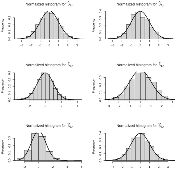
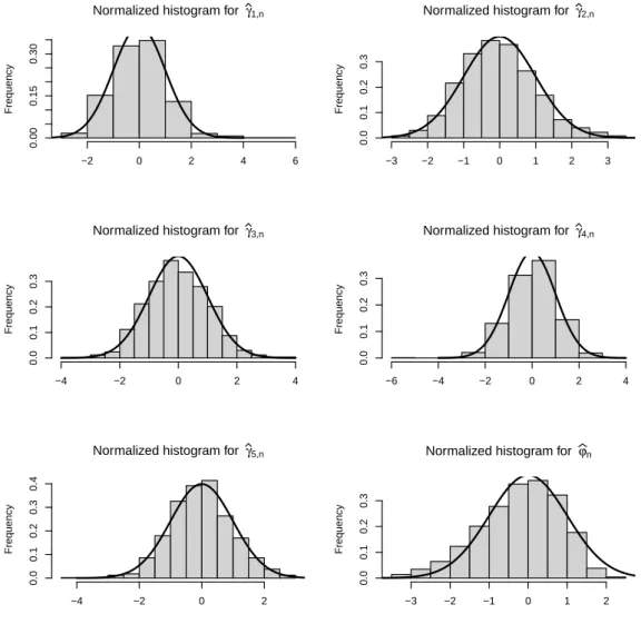
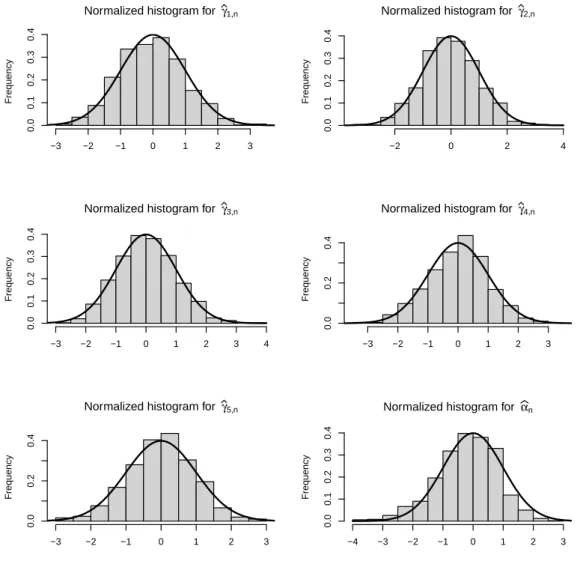
Wald-type confidence intervals are based on approximate normality of parameters estimates. To assess the finite-sample distribution of the MLE, we plot histograms of the normalized estimates ( bβj,n − βj)/ s.e.( bβj,n), j = 1, . . . , 6, (bγk,n− γk)/s.e.(bγk,n), k = 1, . . . , 5, (φbn− φ)/s.e.(bφn) and (bαn − α)/s.e.(bαn), where “s.e.” denotes model-based standard error of the corresponding parameter.
Graphs are provided for a censoring fraction equal to 0.3 (plots for 0.15 yield similar observations and are thus omitted). Histograms for ZIGP (respectively ZINB) model are given by Figures 1 and 2 (respec-tively Figures 3 and 4). On these graphs, the black curve represents the density function of the standard normal distribution. These graphs indicate that the distribution of the MLE can be reasonably approxi-mated by a normal distribution, for every parameter.
Overall, these results suggest that maximum likelihood estimation yields adequate inference on both regression and overdispersion parameters in ZIGP and ZINB models, when censoring is present.
4. Real data application
In this section, we illustrate the censored ZIGP and ZINB models on a real data set from the German Socioeconomic Panel (a survey aimed at investigating healthcare utilization by German households). We also describe a simple and efficient methodology for selecting predictors and interactions in zero-inflation and counts components. Finally, we compare the fitted models using Vuong’s test (a brief reminder of Vuong test is given in Appendix B).
The dataset considered here contains the number of doctor office visits (the response variable) for 1812 West German men aged 25-65 years, during the last three months of 1994. Several risk factors are avai-lable, including age, socio-economic variables : marital status (1 if married, 0 otherwise), educational level (number of years of schooling), household monthly net income (in German marks/1000) and com-position (coded as 1 if children under 16 live in the household, 0 otherwise), two binary variables indica-ting whether individual is covered by a public health insurance and by a supplemental private insurance (both are coded as 1 if yes and 0 otherwise), employment characteristics (coded as self : 1 if self em-ployed, 0 otherwise ; civil : 1 if civil servant ; bluec : 1 if blue collar employee ; employed : 1 if employed), various measures of health status : health satisfaction (health, coded as 0 if low to 10 if high), handicap status (handicap : 1 if handicapped, 0 otherwise) and degree of handicap in per-centage points (hdegree). Following JOCHMANN (2013), who first described these data, we study a
more complex effect of age by considering linear spline variables age30, age35, . . . , age60 (where ageXX is 1 if age ≥ XX and 0 otherwise). Therefore, a total of 20 candidate predictors are available. JOCHMANN (2013) also suggests to consider interactions between health satisfaction and age variables (i.e., age30×health, age35×health, . . . ). There is no reason, however, to limit ourselves to these interactions and one may wish to assess all possible second-order interactions (except for meaningless ones, such as interactions between ageXX variables).
In Figure 5, we plot the number of doctor office visits, censored at 15 visits for illustrative purpose. The plot strongly suggests that data are zero-inflated (41.2% of the observed counts are equal to 0). Thus, we fit the following three models : i) a censored ZIGP model, ii) a censored ZIP model (obtained by letting φ = 1 in [2]) and iii) a censored ZINB model, with all risk factors and second-order interactions, which results in a very large number of possible predictors. Several authors recently addressed variable selection in high-dimensional uncensored ZIP and ZINB models via penalized maximum likelihood, and various penalty functions are implemented in the R package mpath (WANG, 2019). Thus, in a first ap-proximation, we tried to fit penalized ZIP and ZINB models to the healthcare demand data, using all risk factors and interactions and ignoring censoring. None of the methods implemented in mpath converged. Therefore, we propose an alternative methodology for model fitting and variable selection in censored ZIGP and ZINB regressions :
1. First, we determine appropriate predictors for zero-inflation modelling. We fit a logistic regression model to the indicators 1{Zi=0}, i = 1, . . . , n, considered as the response variable. Note that this is not a model for zero-inflation since some of the 0 may arise from the count distribution. However, we may expect that this rough procedure will still identify a relevant subset of predictors, that will be used in a second step in the logistic model for ωi. Given the very large number of potential pre-dictors, we use stepwise logistic regression, starting from a model with no variables (null model). The largest possible model contain all risk factors and interactions. At each step, we use Bayesian information criterion (BIC) to select variables (we prefer BIC to AIC since BIC is generally more parsimonious). Based on this strategy, we select the following predictors : age50 and health. 2. In the second step, we select a preliminary set of predictors for modelling the count component of
the considered zero-inflated model (ZIP, ZIGP or ZINB).
The strategy is the same as above. For example, we use stepwise Poisson regression to select risk factors and interactions that will be used in the count component of the censored ZIP and ZIGP models. Again, variable selection is based on BIC. Starting from the null model, the chosen
predic-tors are age40, age50, handicap, hdegree, health, civil, self, health×hdegree,
civil×age40, self×age40.
We use the same strategy to select a preliminary set of predictors for the count component of ZINB model. The chosen variables are health, age50, self and civil.
3. In the third step, we estimate the censored ZIP, ZIGP and ZINB models defined by logit(ωi) =
γ1+ γ2× age50 + γ3× health and – for ZIP and ZIGP models :
λi = exp(β1+ β2age40+ β3age50+ β4handicap+ β5hdegree+ β6health
+β7civil+ β8self+ β9health×hdegree + β10civil×age40
+β11self×age40) – for ZINB model :
Then we use sequential elimination to obtain the final models. At each step, we remove the less significant predictor, based on Wald test at level 0.01 (if removal decreases the BIC).
Parameter estimates, standard errors and p-values of the corresponding Wald tests are given in Table 5.3. The final models are not nested, thus they are compared using Vuong test (VUONG, 1989). Results are given in Table 5.4.
We now discuss the results of our analysis. First, we observe that the decision of not seeking care is driven by age and health satisfaction. Men aged 50 years and over are less likely to waive doctor visits and the probability of renouncing doctor visits increases with health satisfaction, which is a natural finding. Then, we observe that adding a dispersion parameter has a strong beneficial impact on model fit : comparing censored ZIP and censored ZIGP (respectively ZIP and ZINB) models, Vuong statistic is -9.30 (respectively -9.59) with p-value less than 10−19(respectively 10−21). There is also a large difference between BIC values of final models (7843 for ZIP against 7031 for ZIGP and 7011 for ZINB), which again clearly indicates superiority of ZIGP and ZINB models over ZIP.
Except for handicap, ZIGP and ZINB models select the same risk factors in their count component. Both models indicate higher healthcare utilization by older men (aged 50 or more) and by those having low health satisfaction. Both models also suggest that self-employed (respectively civil servants) have lower healthcare demand than not self-employed (respectively not civil servants). In the German health insurance system, self-employed and civil servants can choose to remain uninsured. The lack of financial compensation may thus explain the fact that these individuals are less likely to visit a doctor. Vuong statistic for comparing ZIGP and ZINB models is -0.85 with p-value 0.40, which suggests that there is no statistically significant difference between the two models. Rather, it is interesting to consider their results jointly. These results confirm the presence of additional overdispersion that is not accounted for by a ZIP model, and give strong evidence of the impact of a few risk factors on healthcare demand.
5. Discussion
In this paper, we investigate MLEs properties in ZIGP and ZINB regression models with right-censored counts. Our simulations suggest that the MLE performs well and that reliable statistical inference on model parameters can be based on the normal approximation of MLEs distribution and on approximation of MLEs variance by Fisher information matrix derived from the censored likelihood.
Variable selection in zero-inflated models is a challenging issue. We observed that variable selection techniques based on penalized maximum likelihood can fail in the uncensored case when the number of possible predictors is too large. Moreover, penalized techniques are currently not available for censored ZI models. Thefore, we propose a simple and efficient strategy for variable selection. This strategy can be implemented using existing softwares.
Our results allow to extend the scope of ZI models to censored data. Now, several issues still deserve attention. For example, random right-censoring is only one of many possible censoring types. In practice, count data may also be left-censored or interval-censored. For now, statistical inference in ZI models in these contexts is an open question. Another question of interest relates to longitudinal data. Here, we are concerned with cross-sectional data but panel data often arise in applications. Extending the current work to the longitudinal setting is therefore of interest and constitutes a topic for our future work.
Appendix A : R code for fitting the censored ZINB model
The code below fits the censored ZINB model to a data set simulated as in Section 3. In this code, b, g and a represent β, γ and α respectively. Functions dnbinom and pnbinom from the R package stats calculate the density and distribution function of the negative binomial distribution (note that these functions use a sligtly different parameterization for the overdispersion parameter). Before running this code, the user needs to specify the design matrices X and W (where each row corresponds to a risk factor and the first rows are made of 1).
The following code builds the censored ZINB loglikelihood : loglikfunZINB=function(param){ b=param[1:p] g=param[(p+1):(p+q)] a=param[p+q+1] sum(delta*J*log(exp(t(g)%*%W)+(1+a*exp(t(b)%*%X))∧(-1/a))+delta*(1-J)* log(dnbinom(z,size=1/a,mu=exp(t(b)%*%X))))+sum((1-J)*(1-delta) *log(1-pnbinom(z-1,size=1/a,mu=exp(t(b)%*%X)))-log(1+exp(t(g)%*%W))) }
The code below determines the initial estimates of β1, . . . , β6, γ1, . . . , γ5 and α and calculates the MLE (intercepts are estimated by default by zeroinfl, thus it is not useful to specify X1 and W1 in the model formula) :
ZINB=zeroinfl(z∼X2+X3+X4+X5+X6|W2+W3+W4+W5,dist="negbin")
ZINBcensored=maxLik(logLik=loglikfunZINB,start=c(unlist(ZINB$coeff), 1/ZINB$theta))
Estimates, standard errors and several other summaries can be obtained using the R function summary.
Appendix B : Vuong test
The principle of the test is as follows. Let f0(·|·) be the true conditional density of Z given (X, W) and
f (·|·, ˆθ) be the estimated conditional density, where ˆθ is an estimate of θ (such as the MLE).
Kullback-Leibler divergence between f0(·|·) and f(·|·, ˆθ) is defined as E0[log f0(Z|X, W) − log f(Z|X, W, ˆθ)], whereE0denotes expectation under the true model.
If two competing models are present, one may choose the one with smallest divergence, since it is closer to the true model. For example, if model 1 is closer to the true model, we have :
where ˆθ(1) and ˆθ(2)are the MLE in models 1 and 2 respectively. Equivalently, E0 [ logf (Z|X, W, ˆθ (1)) f (Z|X, W, ˆθ(2) ] > 0. Let ui = log f (Zi|Xi,Wi,ˆθ(1))
f (Zi|Xi,Wi,ˆθ(2), i = 1, . . . , n. Vuong test statistic is defined as
Z = √n n −1∑n i=1ui √ n−1∑ni=1(ui− ¯un)2 .
Under the null hypothesis H0that models 1 and 2 are equally close to the true model,Z is asymptotically distributed as a standard normal variable. Thus, a decision rule at the asymptotic level α rejects H0 if
|Z| > z1−α2, where z1−α2 is the (1 − α2)-quantile of the standard normal distribution. If Z > z1−α2 (respectivelyZ < −z1−α2), the test chooses model 1 (respectively model 2).
Acknowledgements
Authors acknowledge financial support from the Ministry of Education and Training of the Republic of Vietnam and the French Embassy in Vietnam and logistical support from Campus France (French national agency for the promotion of higher education, international student services, and international mobility).
Bibliographie
BUUA., JOHNSONN. J., LIR., TANX., « New variable selection methods for zero-inflated count data with applications to the substance abuse field. » Statistics in Medicine, n◦30 (2011) : 2326-2340.
CAUDILL, S. B., MIXON, F. G., « Modeling household fertility decisions : Estimation and testing of censored regression models for count data. » Empirical Economics, n◦20 (1995) : 183-196.
CHATTERJEE, S., CHOWDHURY, S., MALLICK, H., BANERJEE, P., GARAI, B., « Group regularization for zero-inflated negative binomial regression models with an application to healthcare demand in Germany. » Statistics in Medicine, n◦37 (2018) : 3012-3026.
CONSUL, P. C., FAMOYE, F., « Generalized Poisson regression model. » Communications in Statistics - Theory and Methods, n◦21 (1992) : 89-109.
CZADO, C., ERHARDT, V., MIN, A., WAGNER, S., « Zero-inflated generalized Poisson models with regression effects on the mean, dispersion and zero-inflation level applied to patent outsourcing rates. » Statistical Modelling, n◦7 (2007) : 125-153.
CZADO, C., MIN, A., « Consistency and asymptotic normality of the maximum likelihood estimator in a zero-inflated generalized Poisson regression. » Collaborative Research Center 386, Discussion Paper 423 (2005) : Ludwig-Maximilians-Universität, München.
FAMOYE, F., WANG, W., « Censored generalized Poisson regression model. » Computational Statistics & Data Analysis, n◦46 (2004) : 547-560.
FENG, J., ZHU, Z., « Semiparametric analysis of longitudinal zero-inflated count data. » Journal of Multivariate Analysis, n◦102 (2011) : 61-72.
HALL, D. B., « Zero-inflated Poisson and binomial regression with random effects : a case study. » Biometrics, n◦ 56 (2000) : 1030-1039.
HE, X., XUE, H., SHI, N.-Z., « Sieve maximum likelihood estimation for doubly semiparametric zero-inflated Poisson models. » Journal of Multivariate Analysis, n◦101 (2010) : 2026-2038.
HENNINGSEN, A., TOOMET, O., « maxLik : A package for maximum likelihood estimation in R. » Computational Sta-tistics, n◦26 (2011) : 443-458.
JACKMAN, S., « pscl : classes and methods for R developed in the Political Science Computational Laboratory. » R package version 1.5.2 (2017) https ://github.com/atahk/pscl/
JOCHMANN, M., « What belongs where ? variable selection for zero-inflated count models with an application to the demand for health care. » Computational Statistics, n◦28 (2013) : 1947-1964.
KARLIS, D., PAPATLA, P., ROY, S., « Finite mixtures of censored Poisson regression models. » Statistica Neerlandica, n◦70 (2016) : 100-122.
LAM, K. F., XUE, H., CHEUNG, Y. B., « Semiparametric analysis of zero-inflated count data. » Biometrics, n◦62 (2006) : 996-1003.
LAMBERT, D., « Zero-inflated Poisson regression, with an application to defects in manufacturing. » Technometrics, n◦34 (1992) : 1-14.
LU, M., LI, C.-S., « Spline-based semiparametric estimation of a zero-inflated Poisson regression single-index model. » Annals of the Institute of Statistical Mathematics, n◦68 (2016) : 1111-1134.
MAHMOUD, M. M., ALDERINY, M. M., « On estimating parameters of censored generalized Poisson regression model. » Applied Mathematical Sciences, n◦4 (2010) : 623-635.
MIN, Y., AGRESTI, A., « Random effect models for repeated measures of zero-inflated count data. » Statistical Modelling, n◦5 (2005) : 1-19.
MOGHIMBEIGI, A., ESHRAGHIAN, M. R., MOHAMMAD, K., MCARDLE, B., « Multilevel zero-inflated negative bino-mial regression modeling for over-dispersed count data with extra zeros. » Journal of Applied Statistics, n◦ 35 (2008) : 1193-1202.
MONOD, A., « Random effects modeling and the zero-inflated Poisson distribution. » Communications in Statistics. Theory and Methods, n◦43 (2014) : 664-680.
MWALILI, S. M., LESAFFRE, E., DECLERCK, D., « The zero-inflated negative binomial regression model with correction for misclassification : an example in caries research. » Statistical Methods in Medical Research 17 (2008) : 123-139. NGUYEN, V. T., DUPUY, J.-F., « Asymptotic results in censored zero-inflated Poisson regression. » Submitted (2018). R CORETEAM, « R : A Language and Environment for Statistical Computing. » R Foundation for Statistical Computing Vienna, Austria (2018) https ://www.R-project.org/
RIDOUT, M., HINDE, J., DEMETRIO, C. G. B., « A score test for testing a zero-inflated Poisson regression model against zero-inflated negative binomial alternatives. » Biometrics, n◦57 (2001) : 219-223.
SAFFARI, S. E., ADNAN, R., « Zero-inflated Poisson regression models with right censored count data. » Matematika, n◦27 (2011) : 21-29.
SAFFARI, S. E., ADNAN, R., GREENE, W., « Hurdle negative binomial regression model with right censored count data. » Statistics and Operations Research Transactions, n◦36 (2012) : 181-194.
SAFFARI, S. E., ADNAN, R., GREENE, W., « Investigating the impact of excess zeros on hurdle-generalized Poisson regression model with right censored count data. » Statistica neerlandica, n◦67 (2013) : 67-80.
TERZA, J. V., « A Tobit-type estimator for the censored Poisson regression model. » Economics Letters, n◦ 18 (1985) : 361-365.
VUONG, Q. H., « Likelihood Ratio Tests for Model Selection and Non-Nested Hypotheses. » Econometrica, n◦57 (1989) : 307-333.
WANG, Z., « mpath : Regularized Linear Models, R package version 0.3-7. » (2019) https ://CRAN.R-project.org/package=mpath
WANG, Z., SHUANGGE, M., WANG, C.-Y., ZAPPITELLI, M., DEVARAJAN, P., PARIKH, C., « EM for regularized zero inflated regression models with applications to postoperative morbidity after cardiac surgery in children. » Statistics in Medicine, n◦33 (2014) : 5192-5208.
WANG, Z., SHUANGGE, M., WANG, C.-Y., « Variable selection for zero-inflated and overdispersed data with application to health care demand in Germany. » Biometrical Journal, n◦57 (2015) : 867-884.
XIE, F.-C., WEI, B.-C., « Diagnostics analysis in censored generalized Poisson regression model. » Journal of Statistical Computation and Simulation, n◦77 (2007) : 695-708.
YEH, H. W., GAJEWSKI, B., MUKHOPADHYAY, P., BEHBOD, F., « The Zero-truncated Poisson with right censoring : an application to translational breast cancer research. » Statistics in Biopharmaceutical Research, n◦4 (2012) : 252-263. ZENG, P., WEI, Y., ZHAO, Y., LIU, J., LIU, L., ZHANG, R., GOU, J., HUANG, S., CHEN, F., « Variable selection approach for zero-inflated count data via adaptive lasso. » Journal of Applied Statistics, n◦41 (2014) : 879-894.
b βn bγn φbn average proportion of censoring βb1,n βb2,n βb3,n βb4,n βb5,n βb6,n bγ1,n bγ2,n bγ3,n bγ4,n bγ5,n 0 bias -0.0114 -0.0002 -0.0001 0.0021 -0.0018 0.0013 -0.0018 -0.0050 -0.0145 0.0104 -0.0019 -0.0257 rel. bias -1.6245 -0.2287 -0.0361 0.2461 0.3685 - 0.2036 0.7627 7.2651 1.5946 - -1.2875 SD 0.1199 0.0256 0.0496 0.0188 0.0365 0.0273 0.2125 0.1320 0.2768 0.1339 0.2377 0.0889 SE 0.1162 0.0251 0.0497 0.0171 0.0352 0.0277 0.2104 0.1311 0.2654 0.1306 0.2399 0.0746 RMSE 0.1673 0.0358 0.0702 0.0255 0.0508 0.0389 0.2990 0.1861 0.3836 0.1873 0.3376 0.1188 CP 0.9470 0.9430 0.9470 0.9390 0.9440 0.9530 0.9530 0.9460 0.9530 0.9440 0.9520 0.9140 ℓ 0.4544 0.0980 0.1946 0.0665 0.1377 0.1085 0.8225 0.5122 1.0362 0.5099 0.9382 0.2916 0.15 bias -0.0107 -0.0010 0.0001 0.0039 -0.0035 0.0012 -0.0121 -0.0099 -0.0144 0.0144 -0.0014 -0.0123 rel. bias -1.5314 -1.0238 0.0172 0.4557 0.6930 - 1.3493 1.5292 7.1805 2.2170 - -0.6169 SD 0.1554 0.0365 0.0717 0.0321 0.0447 0.0378 0.2114 0.1324 0.2826 0.1325 0.2383 0.1034 SE 0.1561 0.0352 0.0719 0.0321 0.0436 0.0381 0.2126 0.1329 0.2670 0.1311 0.2394 0.1024 RMSE 0.2205 0.0507 0.1015 0.0455 0.0626 0.0537 0.3000 0.1878 0.3890 0.1869 0.3377 0.1460 CP 0.9540 0.9410 0.9480 0.9460 0.9410 0.9490 0.9570 0.9460 0.9530 0.9510 0.9520 0.9420 ℓ 0.6114 0.1376 0.2817 0.1259 0.1707 0.1494 0.8315 0.5194 1.0439 0.5123 0.9370 0.3995 0.30 bias -0.0085 -0.0018 -0.0007 0.0059 -0.0029 0.0005 -0.0108 -0.0108 -0.0188 0.0149 -0.0009 -0.0100 rel. bias -1.2103 -1.7514 -0.1696 0.6893 0.5822 - 1.1946 1.6578 9.4151 2.2988 - -0.4993 SD 0.1936 0.0451 0.0956 0.0427 0.0510 0.0477 0.2141 0.1356 0.2875 0.1338 0.2372 0.1581 SE 0.1908 0.0442 0.0915 0.0410 0.0508 0.0471 0.2141 0.1349 0.2717 0.1315 0.2395 0.1546 RMSE 0.2719 0.0632 0.1323 0.0594 0.0720 0.0670 0.3029 0.1915 0.3959 0.1881 0.3370 0.2213 CP 0.9480 0.9490 0.9370 0.9450 0.9450 0.9470 0.9570 0.9450 0.9530 0.9510 0.9520 0.9360 ℓ 0.7465 0.1730 0.3583 0.1603 0.1987 0.1843 0.8373 0.5271 1.0617 0.5134 0.9372 0.5975
Tableau 5.1.:Simulation results for ZIGP model. SD : empirical standard deviation. SE : average standard error. RMSE : empirical root mean square error. CP : empirical coverage probability of 95%-level confidence intervals. ℓ : average length of the confidence intervals.
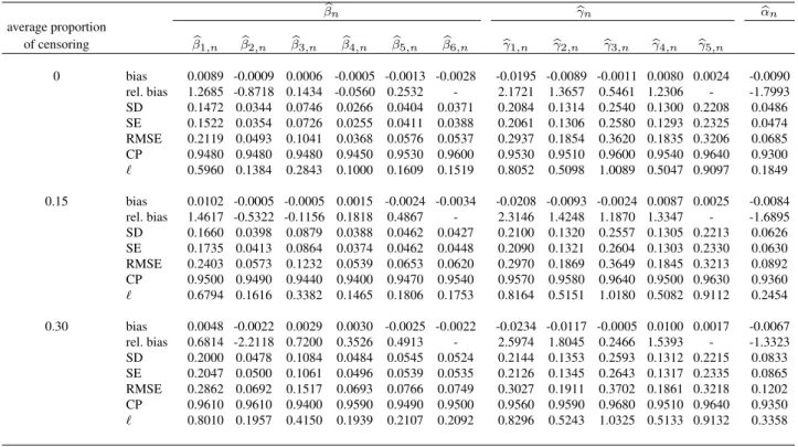
b βn bγn αbn average proportion of censoring βb1,n βb2,n βb3,n βb4,n βb5,n βb6,n bγ1,n bγ2,n bγ3,n bγ4,n bγ5,n 0 bias 0.0089 -0.0009 0.0006 -0.0005 -0.0013 -0.0028 -0.0195 -0.0089 -0.0011 0.0080 0.0024 -0.0090 rel. bias 1.2685 -0.8718 0.1434 -0.0560 0.2532 - 2.1721 1.3657 0.5461 1.2306 - -1.7993 SD 0.1472 0.0344 0.0746 0.0266 0.0404 0.0371 0.2084 0.1314 0.2540 0.1300 0.2208 0.0486 SE 0.1522 0.0354 0.0726 0.0255 0.0411 0.0388 0.2061 0.1306 0.2580 0.1293 0.2325 0.0474 RMSE 0.2119 0.0493 0.1041 0.0368 0.0576 0.0537 0.2937 0.1854 0.3620 0.1835 0.3206 0.0685 CP 0.9480 0.9480 0.9480 0.9450 0.9530 0.9600 0.9530 0.9510 0.9600 0.9540 0.9640 0.9300 ℓ 0.5960 0.1384 0.2843 0.1000 0.1609 0.1519 0.8052 0.5098 1.0089 0.5047 0.9097 0.1849 0.15 bias 0.0102 -0.0005 -0.0005 0.0015 -0.0024 -0.0034 -0.0208 -0.0093 -0.0024 0.0087 0.0025 -0.0084 rel. bias 1.4617 -0.5322 -0.1156 0.1818 0.4867 - 2.3146 1.4248 1.1870 1.3347 - -1.6895 SD 0.1660 0.0398 0.0879 0.0388 0.0462 0.0427 0.2100 0.1320 0.2557 0.1305 0.2213 0.0626 SE 0.1735 0.0413 0.0864 0.0374 0.0462 0.0448 0.2090 0.1321 0.2604 0.1303 0.2330 0.0630 RMSE 0.2403 0.0573 0.1232 0.0539 0.0653 0.0620 0.2970 0.1869 0.3649 0.1845 0.3213 0.0892 CP 0.9500 0.9490 0.9440 0.9400 0.9470 0.9540 0.9570 0.9580 0.9640 0.9500 0.9630 0.9360 ℓ 0.6794 0.1616 0.3382 0.1465 0.1806 0.1753 0.8164 0.5151 1.0180 0.5082 0.9112 0.2454 0.30 bias 0.0048 -0.0022 0.0029 0.0030 -0.0025 -0.0022 -0.0234 -0.0117 -0.0005 0.0100 0.0017 -0.0067 rel. bias 0.6814 -2.2118 0.7200 0.3526 0.4913 - 2.5974 1.8045 0.2466 1.5393 - -1.3323 SD 0.2000 0.0478 0.1084 0.0484 0.0545 0.0524 0.2144 0.1353 0.2593 0.1312 0.2215 0.0833 SE 0.2047 0.0500 0.1061 0.0496 0.0539 0.0535 0.2126 0.1345 0.2643 0.1317 0.2335 0.0865 RMSE 0.2862 0.0692 0.1517 0.0693 0.0766 0.0749 0.3027 0.1911 0.3702 0.1861 0.3218 0.1202 CP 0.9610 0.9610 0.9400 0.9590 0.9490 0.9500 0.9560 0.9590 0.9680 0.9510 0.9640 0.9350 ℓ 0.8010 0.1957 0.4150 0.1939 0.2107 0.2092 0.8296 0.5243 1.0325 0.5133 0.9132 0.3358
Tableau 5.2.:Simulation results for ZINB model. SD : empirical standard deviation. SE : average standard error. RMSE : empirical root mean square error. CP : empirical coverage probability of 95%-level confidence intervals. ℓ : average length of the confidence intervals.
ZIP ZIGP ZINB
parameter estimate std. error p-value estimate std. error p-value estimate std. error p-value Zero-inflation submodel
intercept -2.408137 0.216428 < 2e-16 -2.61000 0.32792 1.73e-15 -2.98345 0.35760 < 2e-16 health 0.300900 0.028496 < 2e-16 0.24136 0.04360 3.11e-08 0.30594 0.04356 2.16e-12 age50 -0.550811 0.122265 6.64e-06 -0.60107 0.22778 0.00832 -0.65075 0.20204 0.001278
Count submodel
intercept 2.286474 0.047607 < 2e-16 2.25776 0.08888 < 2e-16 2.47741 0.09967 < 2e-16 health -0.140050 0.006565 < 2e-16 -0.16361 0.01346 < 2e-16 -0.19345 0.01439 < 2e-16 age40 -0.083821 0.045467 0.065248†
age50 0.234934 0.043893 8.68e-08 0.19988 0.07002 0.00431 0.26571 0.06734 7.94e-05 handicap 0.436929 0.084145 2.07e-07 0.23111 0.07416 0.00183 self -0.233767 0.068345 0.000625 -0.31783 0.11808 0.00711 -0.36536 0.11685 0.001768 civil -0.553545 0.118488 2.99e-06 -0.27089 0.09936 0.00640 -0.38925 0.10194 0.000134 hdegree -0.005052 0.001423 0.000386 civil :age40 0.377772 0.135995 0.005472 φ — — — 1.98527 0.07430 < 2e-16 — — — α — — — — — — 0.68102 0.06884 < 2e-16 BIC 7843.302 7031.811 7011.671
Tableau 5.3.:Summary of final censored ZIP, ZIGP and ZINB models († although not significant, age40 remains in the model because of a significant interaction).
ZIP vs ZIGP ZIP vs ZINB ZIGP vs ZINB
Vuong test -9.30 -9.59 -0.85
p-value < 10−19 < 10−21 0.40
decision ZIGP ZINB equal fit
Tableau 5.4.:Model comparison using Vuong test : Vuong statistic, p-value and test decision (i.e., the best model according to Vuong test).
Normalized histogram for β1,n Frequency −3 −2 −1 0 1 2 3 0.0 0.1 0.2 0.3
Normalized histogram for β2,n
Frequency −3 −2 −1 0 1 2 3 0.0 0.1 0.2 0.3 0.4
Normalized histogram for β3,n
Frequency −2 0 2 4 0.0 0.1 0.2 0.3 0.4
Normalized histogram for β4,n
Frequency −3 −2 −1 0 1 2 3 0.0 0.1 0.2 0.3
Normalized histogram for β5,n
Frequency −2 0 2 4 6 0.0 0.1 0.2 0.3
Normalized histogram for β6,n
Frequency −3 −2 −1 0 1 2 3 0.0 0.1 0.2 0.3 0.4
Figure 1.: Histograms of the normalized estimates ( bβj,n− βj)/s.e.( bβj,n), j = 1, . . . , 6 in censored ZIGP model (30% censoring).
Normalized histogram for γ1,n Frequency −2 0 2 4 6 0.00 0.15 0.30
Normalized histogram for γ2,n
Frequency −3 −2 −1 0 1 2 3 0.0 0.1 0.2 0.3
Normalized histogram for γ3,n
Frequency −4 −2 0 2 4 0.0 0.1 0.2 0.3
Normalized histogram for γ4,n
Frequency −6 −4 −2 0 2 4 0.0 0.1 0.2 0.3
Normalized histogram for γ5,n
Frequency −4 −2 0 2 0.0 0.1 0.2 0.3 0.4
Normalized histogram for ϕn
Frequency −3 −2 −1 0 1 2 0.0 0.1 0.2 0.3
Figure2.:Histograms of the normalized estimates (bγj,n− γj)/s.e.(bγj,n), j = 1, . . . , 5 and (φbn− φ)/s.e.( bφn) in censored ZIGP model (30% censoring).
Normalized histogram for β1,n Frequency −3 −2 −1 0 1 2 3 0.0 0.2 0.4
Normalized histogram for β2,n
Frequency −3 −2 −1 0 1 2 3 0.0 0.1 0.2 0.3 0.4
Normalized histogram for β3,n
Frequency −3 −2 −1 0 1 2 3 0.0 0.1 0.2 0.3 0.4
Normalized histogram for β4,n
Frequency
−3 −2 −1 0 1 2 3
0.0
0.2
0.4
Normalized histogram for β5,n
Frequency
−3 −2 −1 0 1 2 3
0.00
0.15
0.30
Normalized histogram for β6,n
Frequency −3 −2 −1 0 1 2 3 0.0 0.1 0.2 0.3 0.4
Figure 3.: Histograms of the normalized estimates ( bβj,n− βj)/s.e.( bβj,n), j = 1, . . . , 6 in censored ZINB model (30% censoring).
Normalized histogram for γ1,n Frequency −3 −2 −1 0 1 2 3 0.0 0.1 0.2 0.3 0.4
Normalized histogram for γ2,n
Frequency −2 0 2 4 0.0 0.1 0.2 0.3 0.4
Normalized histogram for γ3,n
Frequency −3 −2 −1 0 1 2 3 4 0.0 0.1 0.2 0.3 0.4
Normalized histogram for γ4,n
Frequency
−3 −2 −1 0 1 2 3
0.0
0.2
0.4
Normalized histogram for γ5,n
Frequency
−3 −2 −1 0 1 2 3
0.0
0.2
0.4
Normalized histogram for αn
Frequency −4 −3 −2 −1 0 1 2 3 0.0 0.1 0.2 0.3 0.4
Figure4.:Histograms of the normalized estimates (bγj,n− γj)/s.e.(bγj,n), j = 1, . . . , 5 and (bαn− α)/s.e.(bαn) in censored ZINB model (30% censoring).
0 1 2 3 4 5 6 7 8 9 10 11 12 13 14 15+
Number of doctor office visits
Frequency 0 100 200 300 400 500 600 700