The impact of short selling ban on the CAC40

The impact of short selling ban on

the CAC40

Thesis presented in order to obtain the Bachelor’s degree HES

by :

Fabrice MUDRY

Supervisor :

Geneva, May 31, 2013

Geneva School of Business Administration (HEG-GE)

Business Administration in Banking and Finance

Declaration

This Bachelor’s project has been realized in the framework of the final exam of the Geneva School of Business Administration (HEG) in order to obtain the degree of Bachelor of Sciences in Business Administration with major in Banking and Finance. The student accepts the confidentiality agreement. The author, the Bachelor’s project Supervisor, the juror, and the HEG, without compromising their worth, exclude any responsibility concerning the use of the conclusions and recommendations made.

« I declare that I wrote this thesis myself using the referenced sources.»

Geneva, May 31, 2013 Fabrice Mudry

Acknowledgements

I would like to thank my supervisor François Duc for assisting me in writing this bachelor’s thesis. He has always been available and shared of lot of suggestions. Thanks to his advices and our discursions, I’ve always been expected to go to the next level and progress and as a result I was finally delivering what I consider to be one of my best accomplishments so far.

Executive Summary

This thesis is presented in order to obtain the Bachelor’s degree HES.

The aim of this current thesis is to answer the following question: What are the consequences of the short selling ban enacted from the 12th _{of August 2011 until the}

12th of February 2012 on the CAC40?

In the first part, we define in what consists short selling and describe when it is used. We learn that it is used as a speculative tool when a company is overpriced, it is also used as a hedging technique and it is especially a useful tool to reduce the volatility in a portfolio.

Later we learn about the political context as well as the stock market situation that led the French regulator AMF to the introduction of the short selling ban. The three key moments that triggered the introduction of the short selling ban are the downgrade of America’s AAA credit rating to an AA, the doubt about France’s AAA credit rating and mainly the risk of contagion of the European debt crisis to the countries Spain and Italy. In the second part we make a quantitative analysis with the use of multiple regression analysis to determine the impact on the short selling ban on the stock returns, the volatility, the skewness and the kurtosis.

First we learn that the ban failed to support prices and increased volatility on the restricted stocks. Finally, it deteriorated the price discovery, as the skewness was less negative during the short selling ban. No conclusion can be drawn from our results concerning the occurrence of extreme outcomes because the analysis on the kurtosis were not significant.

Table of contents

Declaration ... i

Acknowledgements ... ii

Executive Summary ... iii

Table of contents ... iv

List of Tables ... vi

List of Figures ... vii

Introduction ... 1

First Part ... 2

1.

  Definition ... 2  

1.1

1.2

2.

  Context of August 2011 ... 6  

2.1

2.2

3.

  Decision of the short selling ban ... 12  

4.

  Literature Review ... 14  

Second Part ... 16

5.

  Methodology ... 16  

5.1

5.2

5.3

5.4

5.4.1   Dependant Variables ... 17   5.4.1.1

5.4.3   Multiple Regression features ... 21  

5.4.3.1

5.4.3.2

6.

  Analysis ... 23  

6.1

6.2

6.3

stocks and of the market ... 29

6.4

7.

  Summary of Results ... 36  

Conclusion ... 38

References ... 39

Annexes ... 40

List of Tables

Table 1: Snapshot of the situation before the introduction of the ban ... 6

Table 2: Retrospective of events before the ban ... 11

Table 3: Geometric Mean of the daily return ... 23

Table 4: Multiple Regression on the return ... 24

Table 5: Annualized Volatility ... 25

Table 6: Multiple Regression on the volatility ... 27

Table 7: Skewness ... 29

Table 8: Multiple Regression on the skewness ... 31

Table 9: Kurtosis ... 33

Table 10: Multiple Regression on the Kurtosis ... 34

Table 11: Arithmetic Average ... 40

Table 12: Robust Multiple Regression on the Return ... 41

Table 13: Robust Multiple Regression on the volatility ... 42

Table 14: Robust Multiple Regression on the volatility with exponential volatility ... 43

Table 15: Robust Multiple Regression on the skewness ... 44

List of Figures

Figure 1: Process of Short selling ... 3

Figure 2: Sharpe Ratio with and without short selling ... 5

Figure 3: Gross Government Debt ... 7

Figure 4: Gross Government Debt ... 8

Figure 5: European Yields go Vertical in 2011 ... 10

Figure 6: Multiple Regression Formula ... 17

Figure 7: Standard Deviation ... 18

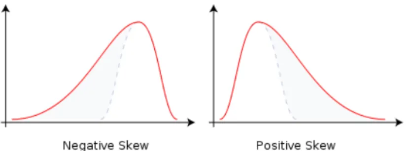
Figure 8: Positive and Negative Skewness ... 18

Figure 9: Formula of Skewness ... 19

Figure 10: Formula of Kurtosis ... 19

Introduction

Short selling has always been portrayed in bad light by the press and has always been criticized when stock prices fall. During the recent crisis we’ve seen a lot of regulatory authorities introducing short selling bans when the prices decrease dramatically.

Yet, there is a lack of theoretical foundation to support this view. On the contrary many research papers tend to confirm that short selling has many benefits. Short selling improves the price discovery, in other words it helps prices reflect more accurately the fundamentals of the company1_{. Ernan Haruvy and Charles Noussair went even further and}

explained in their research2 that “a sufficiently large short selling capacity results in a substantial reduction in the magnitude and duration of bubbles”.

However, the French regulatory body (AMF) decided to introduce a short selling ban in August 2011 as the European crisis became more intense. Unfortunately, regulatory authorities made no comments regarding the expected goal of their action. They have always been vague about the reasons why they put the ban in place. But it seems logical that what the regulatory authorities wished to achieve was primarily an increase of the return of the stock with a decrease of volatility. The previous crisis in 2008 has been analysed and the effectiveness of the ban has already received criticism.

The new short selling ban period offers a new opportunity to analyse the effect of these measures on the stock markets and especially on the restricted stocks. Therefore, the aim of this research paper is to evaluate if this ban has improved or deteriorated the stock market conditions.

1

_{Short Sale Constraints And Stock Returns: Charles M. Jones and Owen A. Lamont (August 2011)}

First Part

1. Definition

1.1 What is short selling?

There is no precise and legal definition of short selling, however, the FSA said that “there is a general understanding in the marketplace that a short sale is a sale of a security that the seller does not own” (FSA, 2002, p.9)3

To further define short selling, there is the first classification made of “explicit” and “implicit” short selling. The implicit short selling is made of the possibility to speculate on the downturn of a stock by the mean of futures, forwards, CDS, options and other derivatives.4

The explicit short selling is the process of selling short the stock directly. We can further classify the explicit short selling into “cover short-selling” and “naked short-selling” 5_.

1. Covered short selling is when the seller has borrowed the securities, or made arrangements to ensure they can be borrowed, before the short sale.

2. Naked or uncovered short selling is when the seller has not borrowed the securities at the time of the short sale, or ensured they can be borrowed.

The problem is that often it is unclear whether the short-selling operation is covered or naked.

According to the press release of the 29 June 2012 of the European Commission, the definition of naked short selling and covered short selling is now more precise. Regulation (EU) No 236/2012 states that short selling of shares can only happen if sellers have either borrowed the shares, have a binding agreement to borrow the shares, or have an arrangement with a third party meaning they can reasonably expect to deliver the shares they are selling.6

4_{http://www.professionsfinancieres.com/docs/2012102306_174_vn_m_short-selling.-need-or-fear.pdf (page3)} 5 _{http://europa.eu/rapid/press-release_MEMO-12-508_en.htm}

In the context of my paper, only the covered explicit short selling is considered. All other types of classifications have only been mentioned as to contextualize and define the scope of the subject of enquiry.

Cover short selling:

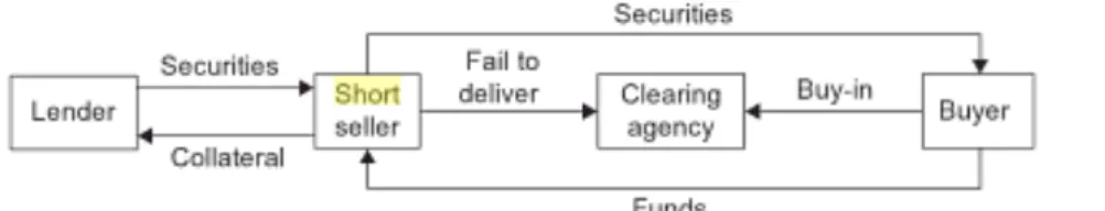
The process of cover short selling means that a broker company will lend a stock to us that we will have to give back in the future. Meanwhile, the borrowed stock is sold and bought back at a certain time later. The investor hopes that the price goes down during the time of the holding. Finally, the stock has to be given back to the brokerage firm. Figure 1 shows the process in detail.

Because the short seller borrows the stock, he has to pay back all dividends or rights declared during the time of the holding. The short-seller borrows the stock; therefore a short interest has to be paid.

Figure 1: Process of Short selling

7

1.2 What is short selling used for?

Because using short-selling means speculating on the fall of the underlying stock price, it might seem counterintuitive to use it. However the use of short selling in a portfolio has many advantages. The mere fact that many governments banned its use during the crises is a proof that it is a common tool used by investors. Below are the three main advantages of short selling and the answer to the question “what is short selling used for?”

Use of short selling:

• As a speculative tool when a company is overpriced

7

• For hedging techniques

• To lower the volatility of a portfolio

1. Speculative tool when a company is overpriced

If you identify that a company is overpriced, you can use the short-selling technique by being short instead of being long. That way, you will profit if the market value of the underlying stock converges to its intrinsic value. During the financial turmoil, all the traders who shorted UBS stocks were expecting to buy it back at a lower price in the future. And so short selling offers opportunity for generating returns even if the market is bearish. 2. Hedging techniques

Short selling allows to hedge against the market risk (beta risk). Considering a portfolio with a massive exposure on the CAC40 market through long positions in the underlying stocks, the portfolio can be hedged in many ways. It can be simply hedged by shorting all the stocks that are contained in the portfolio (partially or totally depending on our view in the evolution of the stocks). Or it can be shorted differently, for instance the investor can short the benchmark index (CAC40 in our example) using exchange traded funds (ETF) or futures. This is an example of how hedge funds managers use a long/short strategy in order to reduce the portfolio’s net market exposure.8

3. To lower the volatility of a portfolio:

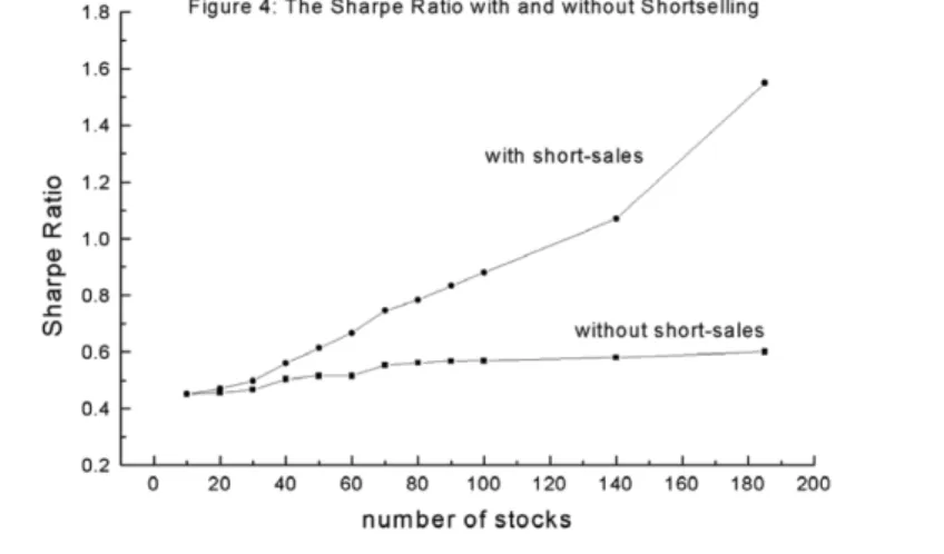
But the most advantageous element of short selling in the management of a portfolio is the risk reduction for each unit of return. Or inversely, short selling allows for a better return for each unit of risk. In other words, short selling allows an optimization of the Sharpe ratio. Short selling is one of the hypotheses of the CAPM theory that draws the efficient frontier line on which lies the portfolio with the highest level of return for its level of risk. In his study “Portfolio Optimization with Many Assets: The Importance of Short-Selling”, Levy and Moshe found out that the proportion of assets held short in mean-variance efficient portfolios converges to 50% as the number of assets increases. So the short selling is a very important part of the portfolio optimization process. In addition, Levy and Moshe

found out that with the constraint of short selling, the cost in terms of risk reduction would be extremely high. For large portfolios, relaxing the constraint can more than double the Sharpe ratio.9 The comparative chart below which contrasts the Sharpe ratio with and without the short-selling constraint illustrates this.

Figure 2: Sharpe Ratio with and without short selling

2. Context of August 2011

2.1 Stock market situation

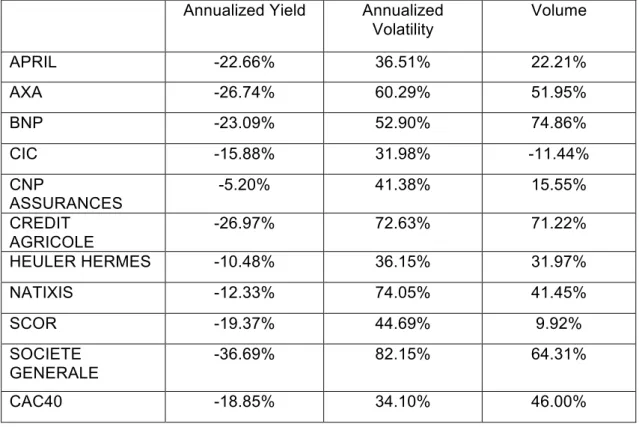
The following table shows the annualized return the month before the ban, the annualized daily volatility of the month before the ban and the increase in the average monthly volume compared to the average volume six months before.

Table 1: Snapshot of the market situations the month before the ban

In August 2011 the 11th, the CAC40 closed at 3149.38 euros. This is more than a 20% decrease in less than a month. The French index had not seen that level since 2009 during the financial turmoil. The daily annualized volatility of the last month approaches 34.10%.

Axa drops 26.74% in less than a month with an annualized daily volatility of 36.51% of the last month. Crédit Agricole drops 26.97% with an annualized daily volatility of 72.63% over the last month. Société Générale drops 36.69% with an annualized daily volatility over 82.15% of the last month.

Annualized Yield Annualized Volatility Volume APRIL -22.66% 36.51% 22.21% AXA -26.74% 60.29% 51.95% BNP -23.09% 52.90% 74.86% CIC -15.88% 31.98% -11.44% CNP ASSURANCES -5.20% 41.38% 15.55% CREDIT AGRICOLE -26.97% 72.63% 71.22% HEULER HERMES -10.48% 36.15% 31.97% NATIXIS -12.33% 74.05% 41.45% SCOR -19.37% 44.69% 9.92% SOCIETE GENERALE -36.69% 82.15% 64.31% CAC40 -18.85% 34.10% 46.00%

In terms of volume the situation increased by more than 46% of trading volume on the CAC40 in comparison to the 6 months before.

2.2 Reasons for the turmoil of 2011

Here are some reasons for the turmoil of 2011:

• Standard & Poor's downgraded America's credit rating from AAA to AA+ on 6th of August 2011 for the first time10_{. The US had an AAA rating since 1941}11_.

• Concerns over France's current AAA rating12.

• Fears of contagion of the European sovereign debt crisis to Spain and Italy.

1. S&P announced on August 5th _{that it would strip the country of its AAA for the first time}

since 1941. Even though rating agencies have lost credibility due to the overstating of the mortgage-backed bonds, the announcement had a huge effect. Indeed, on August 8th_{, the}

first trading day following the announcement, the Dow Jones dropped by 5.5%.

In terms of the timing, the removal of the AAA was odd because in the meantime the Obama administration had to negotiate the increase in the debt ceiling. The explanation of S&P was that in comparison with other AAA countries like Germany or Great Britain, American’s debt, as percentage of annual GDP, was rising unsustainably. As we can see from the picture below, USA’s debt/GDP ratio is much higher and will still be much higher in the future in comparison with the two others countries.

Figure 3: Gross Government Debt

13

2. France’s debt stood at 82% of GDP at that time. This is one of the highest of any AAA-rated country. The market participants were afraid that after the downgrade of the USA by the S&P rating agency on August 5th, it was now France’s turn to suffer a downgrade. Therefore on August 10th _{rumours and panic invaded the market places. French President}

Nicolas Sarkozy rushed back from his holiday to defend the country from financial attack. On the same day Société Générale fell by almost a fifth before recovering some ground to close down 15%. BNP Paribas fell by 9.5% whereas Crédit Agricole fell by 12%. The reasons why French banks reacted so intensely are that they had exposure to Greece, Italy and of course France. So it became very dangerous to hold French financial stocks in a portfolio.

3. According to the Maastricht criteria, the ratio of the annual government deficit to GDP must not exceed 3% at the end of any given year. And the debt to GDP ratio must not exceed 60% at the end of the preceding fiscal year. But as we can see in the following graphic, none of the major European countries respected it.

Figure 4: Gross Government Debt

The 17 Euro-zone countries have in common the use of the Euro currency, however they do not share any fiscal policy integration. This is the major difference between the USA and the Euro-zone. This is problematic when the countries inside the same currency areas grow at different levels, as it was the case in Europe.

Greece and Ireland that are much smaller countries already had difficulties and needed the help of the European Union. The problem worsened when the financial difficulties

impacted Spain and Italy which are much bigger countries. As a consequence those governments bonds yields near 6% to 7% which is simply unsustainable. The ECB didn’t want to intervene, as it is not coherent with inflation stability which is the first priority of the ECB. Meanwhile the politicians couldn’t come up with a solution.

Finally, politicians put enough pressure on the ECB to make them intervene. For the first time in the history of the ECB, the Central Bank began buying Italian and Spanish bonds in an effort to stop the sovereign-debt crisis on the August 8th.

The initial reaction was positive and the CAC40 rose 1.1% on August 8th _{(previous trading}

day on August 5th_{: -8%). That reaction of the European Central Bank brought each}

country’s ten-year yields down by around a percentage point on August 8th over Germany. But this was only temporary; indeed the stock market dropped again the following day by almost 4%.

Figure 5 shows the evolution of the European Yields on the main countries in Europe. Since the introduction of the Euro as a currency, the interest rates converged to reach a common line between 2001 and 2009. After the Lehman Bankruptcy, the rate of Germany and France decreased whereas the rate of all the other countries increased. This graph also shows the reaction of the interest rate as of August 2011 when the ECB intervened. All the interest rates dropped.

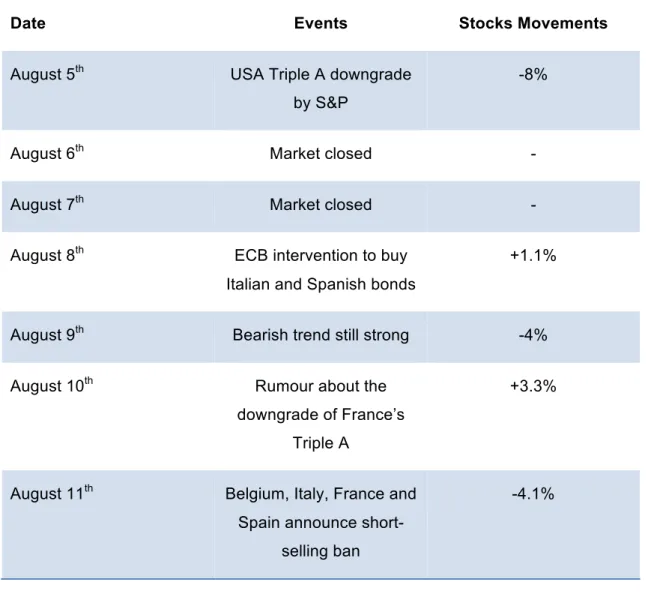
Table 2 provides a reconstitution of the main events that took place the week before the short selling ban.

Table 2: Retrospective of events before the ban

Date Events Stocks Movements

August 5th USA Triple A downgrade

by S&P

-8%

August 6th _{Market closed -}

August 7th _{Market closed -}

August 8th _{ECB intervention to buy}

Italian and Spanish bonds

+1.1%

August 9th _{Bearish trend still strong -4%}

August 10th Rumour about the

downgrade of France’s Triple A

+3.3%

August 11th _{Belgium, Italy, France and}

Spain announce short-selling ban

3. Decision of the short selling ban

This is in the context where four European countries announced a short-selling ban on August 11th. Belgium, France, Italy and Spain announced a short-selling ban on a total of 59 stocks14_{. Ireland still had a short-selling ban on the financial stocks since September}

200815. Turkey and Greece16 imposed a short-selling ban on August 8th. These measures were lifted first by the French government on the 11th _{of February 2012 (six month later)}

and last by the Italian government on the 24th _{February 2012.}

In this paper we study the case of France and the 10 stocks that were concerned by the short-selling ban. Initially, the AMF (Autorité Française des Marchés) imposed a ban only during 2 weeks that lasted until the 25th _{of August, it was then prolonged until the 29}th _of

September, and again until the 11th _{of November and was finally lifted on the 11}th _of

February 2012. The short-selling ban in France concerns the following ten stocks: • April Group • AXA • BNP Paribas • CIC • CNP Assurances • Crédit Agricole • Euler Hermès • Natixis • Scor • Société Générale

Those four countries have put this measure in place after a very turbulent week on the market place. However not all the European countries saw the benefit in the introduction of a short-selling ban. Britain, the Netherlands and Austria said they saw no need for action,

while Germany said it would instead\rather push for a Europe-wide ban on a so-called naked short selling17.

Such measures were already taken in 2008 during the Lehman Brother collapse. 799 American institutions were banned from short selling and most of the countries with a solid financial system followed the move by instating a short-selling ban. During that time lots of researches have been written about the effect of short selling on the stocks markets. Now we will review the literature that has been written and what we have learned from the 2008 short-selling ban.

4. Literature Review

The crisis of 2008 has been the foundation for a lot of research related to the short selling ban. The kind of research that have been performed are diverse. Most research seeks to analyse the impact of short selling ban on the return, the price discovery (or the process used in determining spot prices through supply and demand), the volatility or the distribution characteristics of the stocks. There are also many studies which focused on the market liquidity but this is not the object of our studies.

LISA A. SCHWARTZ and KATI D. NORRIS made a comparison between the restricted financial stocks and the non-restricted financial stocks during the short selling ban period of 2008. In addition it divided into small, medium and large market capitalization firms to analyse the effects of size. Restricted and non-restricted firms suffer declines in returns during the ban and an increase in their volatility level. The restricted firms saw their skewness increase in positive territory. In terms of the volatility, ABRAHAM LIOUI (2009) shows that the short-selling ban was followed by a rise in the volatility of the markets and that the risk/reward had worsened18.

The work of PEDRO A. C. SAFFI AND KARI SIGURDSSON is very interesting because they reached the same conclusion, but starting from another perspective. They used the annual average lending supply and loan fees to measure the degree of short-sale constraint. They found that firms with higher lending supply and lower short-selling constraints have a higher degree of negative skewness and lower levels of volatility.19 They also found that the price efficiency is affected by a high short-sale constraint, since limited lending supply are associated with lower efficiency. One of the major studies that has been made is the one from BEBER AND PAGANO (2010). They also analysed the data of 16491 stocks in 30 countries from January 2008 to June 2009 and found that the bans were detrimental for liquidity, (ii) slowed down price discovery, especially in bear market phases, and especially (iii) failed to support stock prices, except possibly for U.S. financial stocks.20

18  http://msc-­‐financial-­‐markets.edhec.com/servlet/com.univ.collaboratif.utils.LectureFichiergw?ID_FICHIER=1328885973188 19  http://papers.ssrn.com/sol3/papers.cfm?abstract_id=949027

20

BAI, CHANG AND WANG (2006) show that constraining short sales reduces markets allocation and informational efficiency by limiting trades for risk-sharing and private information. These two effects drive market prices in opposite directions but if the information effect is significant, short-sale constraints can actually cause prices to decrease and to be more volatile.21 _{COPELAND explains that a short-selling ban worsens}

the price discovery by hindering the negative opinion to be reflected in the price. In others words, the « no voters » are not in the currently quoted price. ARTURO BRIS, WILLIAM N. GOETZMANN, AND NING ZHU found some evidence that prices incorporate negative information faster in countries where short sales are allowed and practiced, so that the price efficiency is better without short-selling ban. They found strong evidence that in markets where short selling is either prohibited or not practiced, market returns display significantly less negative skewness.22

BOEHMER, JONES AND ZHANG (2009) made a research on the September 2008 short-selling ban on the US market and concluded that the shorting activity drops by 77% in large-cap stocks, stocks prices appear unaffected by the ban and that most of the firms suffer a severe degradation in market quality, as measured by quoted spreads, effective spreads and volatility.23 ARTURO BRIS (2008) found that the market quality, measured through the quoted spread, relative spread and the price range is significantly worse for the stocks that were affected by the short-selling ban compared to other comparable stocks.24

csefwp/241.html.

21 _{http://web.mit.edu/wangj/www/pap/BCW_061112.pdf} 22

http://www.arturobris.com/index_files/bear.pdf 23

Boehmer,  E.,  Jones,  C.,  &  Zhang,  X.  (2009).  Shackling  short  sellers:  The  2008  shorting  ban.  Working   Paper,  Cornell  University,  Ithaca,  NY.  Retrieved  from  http://papers.ssrn.com/sol3/papers  

.cfm?abstract_id=1412844.

Second Part

5. Methodology

In this section, I will explain the model I used to measure the impact of short-selling ban on the stocks markets. My model is inspired by the model of Abraham Lioui in his research paper called « The Undesirable Effects of Banning Short Sales » of April 2009. It shows how the markets responded negatively to the short-selling ban on the restricted stocks in France in the period of the short-selling ban in 2008.

5.1 Description of the time frame

The data has been downloaded from Yahoo Finance. Yahoo Finance is considered one of the best free data supplier on the market. All the collected data are adjusted for dividends payment and any splits that could have happened. My research covers the time period between May 25th 2010 until February 12th 2012. The study has three distinct time frames. First there is the pre-crisis period that goes from May 25th 2010 until February 18th 2011. Then the crisis period that goes from February 18th 2011 until September 22th 2011. Finally, the short-selling ban goes from August 12th 2011 until February 2012. The sample size for each stock and index is 418 trading days. The number of observations is important to take into consideration because we used multiple regression analysis with three explanatory variables. It is commonly said that for each explanatory variable we should have twenty observations so in our case, it is respected.

The short-selling ban period is simply the official period in which the ban was active under the governance of the AMF. To help define the better pre-crisis and crisis period, we first pre-define a time horizon identical with the short-selling ban period. We then tested, by iterative search some specific key points to find where we had the more consistent and clear results.

5.2 Description of the data set

The short-selling ban was effective for 10 stocks on the French indexes; we thus made the same calculations on all these stocks. All the stocks are traded on the CAC Family but not

all are traded in the CAC40. To make a comparison we use five indexes: CAC40, DAX, FTSE, NASDAQ and the S&P500.

The CAC40 is the only index where some stocks were prohibited from short selling. We can thus make a comparison between the stocks that were prohibited from short selling and the benchmark CAC40. In addition we can also make a comparison with other indexes where no short selling ban had been active during this time. These comparisons help draw some conclusions concerning reasons for the changes.

5.3 Description of the equipment

Finally to help us make all the calculations we used the two programs Excel and SPSS. Excel is easy to use, customizable and especially, it is compatible with other financial and data manipulation and was thus used for many calculations. It has been used among others to transfer the raw data from Yahoo Finance to an Excel sheet. Excel was used to make all the basic calculations.

SPSS on the other hand offers a more effective way to manage data, it offers a wider range of options and above all shows a better output organization. That is very advantageous in the context of our research paper because a massive amount of data is being used, transformed and analysed. So in this context, SPSS was of great utility and was used among others for the computation of the multiple regression analysis. SPSS offers to choose many optional statistics tests (for example the collinearity test) and offers more customizable features for our test such as the possibility of removing the constant.

5.4 Multiple Regression Analysis

The multiple regression analysis is a statistical measure that attempts to determine the strength of the relationship between one dependent variable (usually denoted by Y) and a series of other changing variables (known as independent variables).

Figure 6: Multiple Regression Formula

Multiple Regression: Y = a + b1X1 +b2X2 + B3X3 + ... + BtXt + u

5.4.1 Dependant Variables

We have run multiple regressions on the performance, the volatility, the skewness and the kurtosis.

5.4.1.1 Performance

The performance is measured as the average return of the last sixty days.

5.4.1.2 Volatility

The volatility is measured as the standard deviation of the returns. Volatility is a measure of dispersion. In statistical terms, the standard deviation is the squared root of the average squared deviations from the random variable’s expected value.

Figure 7: Standard Deviation

Where σ is the standard deviation, xk represents each value in the data set, µ is the mean

of all the observation and n is the number of observations.

Volatility is the most common risk measure despite its imperfection. The two most important imperfection of the volatility as a measure of the risk are:

• Upside price movement are considered as risky as the downside price movement • Volatility is estimated with past price movement

For the multiple regression analysis, we computed the volatility as the average daily volatility of the last sixty days.

5.4.1.3 Skewness

In finance, skewness is the measure of the symmetry of the return distribution. Skewness can be “positive” or “negative”. A “positive” skewness is skewed to the right whereas a “negative” skewness is skewed to the left. Skewness is a measure of downside risk.

Statistically, skewness of a random variable X is the standardized third moment. If the result of the computation is greater than zero, the distribution is positively skewed. If it's less than zero, it's negatively skewed. A normal distribution has a skewness of zero.

Figure 9: Formula of Skewness

Where µ is the mean, σ is the standard deviation, X is a random variable and E is the expectation operator.

Skewness informs us about the spreading out of the distributions. A negative skewness means that the spread between all the data in the negative territory is wider than in the positive. The same goes for the positive skewness but on the positive territory.

For our multiple regression analysis, the skewness is computed as the average daily skewness of the last sixty days.

5.4.1.4 Kurtosis

The kurtosis analyses the occurrence of extreme movements. It is a measure of the “peakedness” of the probability distribution and helps describe the shape of a probability distribution. Statistically kurtosis is the standardized fourth moment.

Figure 10: Formula of Kurtosis

Where µ is the mean, σ is the standard deviation, X is a random variable and E is the expectation operator. As we could expect, the kurtosis rose during the crisis.

Figure 11: General Form of Kurtosis

The mesokurtic distribution has a kurtosis of three (or an excess kurtosis of zero). The most common example of a mesokurtic distribution is the normal distribution. The leptokurtic distribution has a kurtosis more than 3 (or an excess kurtosis more than 0) a more acute peak around the mean and fatter tails; it has thus more probability of extreme movements. The platykurtic has a kurtosis smaller than three (or negative excess kurtosis) and has a lower, wider peak around the mean and thinner tails.

For our multiple regression analysis, the kurtosis is computed as the average kurtosis of the last sixty days.

5.4.2 Independant Variable

5.4.2.1 Dummy variables

The aim of our multiple regression analysis is to differentiate the effect of the short selling ban from those of the financial crisis. To capture the effect of the financial crisis and the short selling ban we use two dummy variables.

5.4.2.2 Lag volatility

In time series analysis, lag volatility is often used to avoid bias. This allows varying amounts of recent history to be brought into the forecast. We are aware that adding a lagged variable can damage the results of the multiple regression by dominating the others explanatory variables. However our independent variables do not exhibit a high serial correlation and a heavy trending in exogenous variables so our result should not suffer. The use of a lagged variable as an explanatory variable makes our results very persistent and lead to an R^2 close to 1. This is the reason why we do not show it.

5.4.2.3 Market Fluctuations

To capture the market fluctuation, we added the benchmark return as an explanatory variable. For all the banned stocks, we added the CAC40 index return which can be considered as the benchmark, since every stock is part of the CAC Family. For each index, we add their own return as the benchmark.

5.4.3 Multiple Regression features

5.4.3.1 Intercept:

Our model does not contain any intercept. The dummy variables are explicitly explained in the equation and therefore the risk of collinearity may appear.

5.4.3.2 Robustness

For each of our multiple regression analysis, we computed a robust model that we put at the end. The goal of the calculation of the robust model is to capture two additional economic environments.

We added a TED Spread which is aimed to capture liquidity issues. The TED Spread is the spread between the LIBOR rate and the T-bill rate. The T-bill rates are considered risk-free whereas the LIBOR is the interest rate paid on interbank deposits in the international money markets commonly used as a benchmark for short-term interest rates. The data was collected from the official Internet website of the FED.

We added the CREDIT Spread that measures the default premium. The Credit Spread is defined as the difference in yield between an AAA-rated company and a BAA-rated company. As for the TED Spread, the Credit Spread data were collected on the Fed’s official website.

Abbreviations of variables:

Coeff lag: Coefficient of the lag variable.

Coeff index: Coefficient of the CAC40 for the restricted stock. Coeff Crisis: Coefficient of the crisis (dummy variable).

Coeff Short: Coefficient of the short selling ban (dummy variable). T-stat lag: T-statistic of the lag variable.

T-stat index: T-statistic of the CAC40 for the restricted stock. T-stat Crisis: T-statistic of the crisis (dummy variable).

6. Analysis

6.1 The impact of the short selling ban on the performance of the

banned stocks and of the market

Table 3: Geometric Mean of the daily return

This table is very clear as we notice that during the period of the pre-crisis, the indexes as well as the stocks all show positive results. This confirms that this period was an uptrend on the stock markets. During the crisis, we see again that the stocks and the indexes are negative, however it is interesting to point out that the stocks dropped a lot more than the indexes. What the indexes tell us is that the DAX and the CAC40 dropped two to three times as much as the American indexes, this is the result of the European crisis that made the stock indexes of Europe suffer more. Finally, during the short-selling ban, all indexes switched trends by increasing again even though we notice a weak trend for the CAC40 with only 0.04% increase. Whereas all indexes switched sign during the period of the

Pre-crisis Crisis Short selling ban

CAC 0.09% -0.26% 0.04% DAX 0.13% -0.24% 0.09% FTSE 0.08% -0.13% 0.08% NASDAQ 0.10% -0.08% 0.12% S&P500 0.09% -0.10% 0.10% APRIL 0.01% -0.39% 0.01% AXA 0.08% -0.38% 0.10% BNP 0.12% -0.58% -0.05% CIC 0.14% -0.24% -0.17% CNP ASSURANCES 0.05% -0.20% -0.23% CREDIT AGRICOLE 0.17% -0.67% -0.17% HEULER HERMES 0.18% -0.28% -0.05% NATIXIS 0.08% -0.46% -0.25% SCOR 0.17% -0.17% 0.19% SOCIETE GENERALE 0.21% -0.77% -0.04%

short-selling ban, suggesting that the introduction of the short selling ban has been effective, the situation is different with the stocks. Indeed, seven out of ten stocks further decreased during the period with sometimes even very large losses. Natixis, CNP Assurance and Credit Agricole dropped respectively -0.25%, -0.23% and -0.17% on a daily average during that period. It is an interesting picture because Europe was in crisis, the indexes increased after the introduction of the short selling ban but not the restricted stocks. The downtrend seemed however to have slowed down. By mean of comparison, we computed the arithmetic mean of the daily return that we put in the appendix25. We cannot however draw a definitive conclusion out of this Table

.

Table 4: Multiple Regression on the return

The Coefficient of the crisis and the short selling ban confirm the trend what we have on the last table. The stocks went down during the crisis and still went further down during the

25

See annex Table 11

COEFF LAG COEFF INDEX COEFF CRISIS COEFF SHORT T-STAT LAG T-STAT INDEX T-STAT CRISIS T-STAT SHORT CAC 0.97 0.01 -0.00 0.00 89.07 16.44 -1.46 0.27 DAX 0.97 0.01 -0.00 0.00 113.14 16.95 -1.41 0.53 FTSE 0.97 0.02 -0.00 0.00 98.92 16.79 -1.12 0.51 NASDAQ 0.97 0.02 0.00 0.00 105.79 18.30 -1.04 0.46 S&P500 0.97 0.02 -0.00 0.00 107.02 18.06 -1.21 0.59 APRIL 0.97 0.01 -0.01 0.00 91.29 7.02 -2.47 0.57 AXA 0.97 0.02 -0.01 0.00 81.90 13.75 -0.88 0.12 BNP 0.96 0.02 -0.01 -0.01 73.95 12.75 -1.11 -0.77 CIC 0.98 0.01 -0.00 -0.00 99.69 5.29 -1.35 -0.42 CREDIT AGRICOLE 0.98 0.02 -0.01 -0.00 92.74 12.37 -1.29 -0.42 EULER HERMES 0.96 0.01 -0.01 -0.00 70.86 7.90 -1.50 -0.72 NATIXIS 0.96 0.02 -0.01 -0.01 72.45 11.86 -0.98 -1.30 SCOR 0.96 0.01 -0.01 0.01 81.19 9.88 -1.33 1.48 SOCGENERALE 0.97 0.02 -0.01 -0.00 84.27 11.90 -1.55 -0.03 CNPASSURANCES 0.97 0.01 -0.01 -0.00 77.97 10.42 -1.29 -0.79

short selling ban. As we can see, no result is significant during the short selling ban. Thus, we fail to reject the null hypothesis that “the short selling ban has an impact” on the return of the restricted stocks. However, we observe that the trend is very clear on the last table and it is confirmed by the coefficient on the multiple regressions. All in all this is a strong indication of a relationship even though the results are not significant.

6.2 The impact of the short selling ban on the volatility of the

banned stocks and of the market

Table 5: Annualized Volatility

The five indexes that we measured increased their volatility during the crisis whereas eight

out of ten stocks increased their volatility during that time. During the short-selling ban the volatility of all indexes still increased further but it is interesting to note how volatile the CAC40 and the DAX indexes were. The CAC40 has an annualized volatility of 28.07% and the DAX has a volatility of 28.97%. It is probably related to the European crisis which affected the EU more than the other countries. The volatility of the stocks increased for all of them without exception and it is important to emphasize that some stocks have known

Pre-crisis

Crisis

Short selling ban

CAC 19.92% 28.075 35.42% DAX 15.61% 28.97% 36.04% FTSE 15.99% 21.64% 24.37% NASDAQ 18.68% 26.28% 27.25% S&P500 16.75% 23.91% 25.24% APRIL 32.20% 31.24% 36.99% AXA 35.04% 48.63% 71.49% BNP 35.67% 53.40% 58.29% CIC 19.21% 21.75% 29.31% CNP ASSURANCES 28.19% 34.27% 45.67% CREDIT AGRICOLE 42.35% 54.79% 80.26% HEULER HERMES 32.42% 27.25% 39.50% NATIXIS 37.24% 49.03% 74.42% SCOR 21.17% 34.35% 41.88% SOCIETE GENERALE 44.52% 59.79% 93.81%

some period of great volatility. Five of them even had an annualized volatility above 45%. Even though every stock experienced a systematic increase in volatility, the increase was not the same for all. Some stocks increased dramatically, for example, BNP Paribas rose from 35.67% during the crisis to 53.40% during the short-selling ban, and Societe Generale rose from 44.52% during the crisis to 59.79% during the short selling ban. On the other hand April only rose from 32.20% to 31.24% whereas CIC only rose from 19.21% to 21.75%.

We see that the volatility increased during the pre-crisis period, it increased even more during the short selling ban period. We also notice that the increase was more powerful for the restricted stocks than the indexes. Because the volatility of the indexes also rose, it shows that it is not only because of the short selling ban but also probably because of market wide factors.

Table 6: Multiple Regression on the volatility

This multiple regression analysis is very interesting as it shows how important and linked the increase in volatility and the crisis were. During the crisis, all indexes and eight out of ten stocks have positive and significant results. Euler Hermès is not significant and this confirms the previous result because it is the only stock whose volatility decreased during the crisis time period. Very oddly we noticed that the effect of the crisis was stronger on the indexes than on the stocks.

But what is very interesting to look at is the effect of the short-selling ban on the volatility. What this table shows is that for the indexes, the short selling ban is not significant. This means that the volatility didn’t decrease significantly in the markets with the introduction on the short-selling ban. To further analyse the case of the indexes, we see a large difference between the two American indexes NASDAQ and the S&P500 which illustrates a negative relationship with the volatility during the time of the short selling ban. It is consistent with the past result of the historical volatility where we can see that for these two indexes, there were almost no changes during the crisis and the short-selling period. This again demonstrates that the crisis was a European one and that the USA did not suffer too much collateral damage. COEFF LAG COEFF INDEX COEFF CRISIS COEFF SHORT T-STAT LAG T-STAT INDEX T-STAT CRISIS T-STAT SHORT CAC40 0.99 0.00 0.02 0.00 625.03 -0.55 4.82 1.32 DAX 0.99 0.00 0.02 0.00 597.04 -0.63 6.71 1.19 FTSE 0.99 0.00 0.01 0.00 697.04 -0.53 5.36 0.26 NASDAQ 0.99 0.00 0.02 -0.01 598.66 -2.00 4.83 -1.59 S&P 0.99 0.00 0.01 -0.01 566.17 -2.47 4.92 -1.62 APRIL 0.99 0.00 0.01 0.00 647.42 -0.35 2.14 0.54 AXA 0.99 0.00 0.03 0.02 585.47 0.58 4.26 1.79 BNP 0.99 0.00 0.03 0.03 505.71 0.84 4.38 2.34 CIC 0.99 0.00 0.00 0.00 491.34 -0.12 2.04 1.34 CREDIT AGRICOLE 0.99 0.00 0.02 0.01 515.56 1.44 3.39 0.91 EULER HERMES 0.99 0.00 0.00 0.01 690.32 0.04 0.89 2.15 NATIXIS 0.99 0.00 0.03 0.02 502.00 0.07 3.92 1.83 SCOR 0.99 0.00 0.03 0.02 489.57 -0.02 3.59 1.29 SOCGENERALE 0.99 0.00 0.03 0.04 114.55 -0.04 3.15 1.93 CNPASSURANCE 1.00 0.00 0.00 0.01 602.08 1.43 0.95 1.50

Concerning the stocks, the situation is even worse as the results of four stocks out of ten are still significant during the short selling ban. As a result, we can reject the null hypothesis that “the short selling ban had no impact on the volatility”. This signifies that the introduction of the short-selling ban increased with great significance the volatility on the restricted stocks. The results are consistent with the past results. We see that the stocks whose results are significant for the short selling ban period, are those who see their annualized volatility increase the most in the past results.

In order to capture two additional economic environments, we computed a robust multiple regression analysis26_{. We found similar results with the robust form. We notice that the}

results of the restricted are even more significant when we consider other variables. It is also interesting to notice that the CREDIT Spread is significant five times out of ten. The CREDIT Spread measures the probability of default and thus it is consistent with our result because there was a high probability of default on some financial institutions.

The above results are very interesting because they show how the regulatory authorities failed to reduce the volatility on the markets. The volatility increased significantly during the crisis and the short selling ban for almost all the stocks. Fear could be an explanation for the market behaviour, but I think that above all this shows that the markets participants did not trust the regulatory authorities’ interventions.

We also made the same calculation with an added explanatory variable in the form of exponential variability27_{. The results are completely different and not very consistent with}

the past results. One reason for that might be the fact that the lagged variable and the exponential variable are too dominant in comparison with all the others variables. These results might be biased and this is the reason we don’t analyse further here.

The t-stat result of the lagged volatility is highly significant as it is often the case with lagged variables.

See Figure 13 in the annex

27

6.3 The impact of the short selling ban on the skewness of the

banned stocks and of the market

Table 7: Skewness

The previous results informed us of the increase in volatility of the indexes and the stocks during the financial crisis and the short selling ban. Now the study of the skewness aims to inform us on the direction of this movement.

Skewness informs us about the spreading out of the distributions. As such, the skewness is a measure of the downside risk. These results will inform us if the skewness is positive or negative and thus, on what side our distribution of returns “leans”.

Table 7 shows very clear and distinct results. During the crisis the skewness dropped for the indexes and the stocks. Indeed the only exception to this decrease is Natixis. It rose from -0.68 to 0.18. During the short selling ban period, every index increased its skewness

Pre-crisis

Crisis

Short selling ban

CAC -0.03 -0.63 -0.05 DAX 0.04 -0.51 -0.05 FTSE 0.03 -0.44 -0.13 NASDAQ -0.22 -0.41 -0.07 S&P500 -0.02 -0.63 -0.16 APRIL 0.01 -0.30 -0.57 AXA 0.26 -0.50 0.23 BNP 0.14 0.07 0.37 CIC 0.77 -0.78 0.53 CNP ASSURANCES 0.37 -0.07 0.39 CREDIT AGRICOLE 0.38 -0.74 0.53 HEULER HERMES 0.35 -0.78 0.46 NATIXIS -0.68 0.18 0.33 SCOR 0.37 -0.35 -0.01 SOCIETE GENERALE 0.47 -0.87 0.32

whereas only one stock decreased. Indeed only April decreased from -0.30 to -0.57. This result confirms the research paper of Lisa A. Schwartz and Kati D. Norris28. They found out that during the short selling ban of 2008, “the restricted firms showed an increase of the skewness in the positive direction”.

During the short- selling ban only April is negatively skewed and Scor is symmetrical with a value of zero. Every other stock is showing a positive skewness. All in all, when we consider the situation in the pre-crisis period and during the short selling ban period, the situation is more ambiguous. Indeed four indexes out of five have dropped but their value is very similar. Five stocks out of ten decreased whereas four stocks out of ten rose. From these results we see a very consistent trend with skewness leaning to the left (on the negative territory) during the financial crisis and then switching sign during the short selling ban to lean on the right. This has always been seen better in the view of the investor to have a skewness leaning to the right than to the left. To confirm this positive outcome we run a multiple regression on the skewness on the next table.

28 _{The Impact of Temporary Short Selling Restrictions on the} Volatility of Financial Stock Prices: Does Firm Size Matter?

Table 8: Multiple Regression on the skewness

This table confirms the trend from the last results. The coefficients of the financial crisis are almost all negative for the indexes and the restricted stocks with the exception of two stocks (Natixis shows a positive coefficient and confirms the last result with an increase of the skewness during the financial crisis). The coefficients of the short selling ban are all positive except for APRIL which also precedently exhibits a decrease of the skewness. We see that the effects of the short selling ban seemed to have been stronger on the restricted stocks. No index has significant results whereas AXA, CREDIT AGRICOLE and CNP ASSURANCES have significant results with respectively 2.29, 2.03 and 1.97. These three stocks also had the biggest swing in their skewness in the past results. Among the stocks that had bigger swings in their skewness there was also EULER HERMES and SOCIETE GENERALE and based on the multiple regressions, we see that their results are almost significant with 1.84 T-STAT each. This means that we can reject the null hypothesis that “the short selling ban had no impact on the skewness”.

COEFF LAG COEFF INDEX COEFF CRISIS COEFF SHORT T-STAT LAG T-STAT INDEX T-STAT CRISIS T-STAT SHORT CAC40 0.96 0.00 -0.01 0.01 94.01 1.06 -1.15 1.16 DAX 0.95 0.01 -0.01 0.01 62.37 3.33 -1.22 1.62 FTSE 0.95 0.00 -0.01 0.01 68.84 1.23 -1.44 0.83 NASDAQ 0.97 0.01 -0.01 0.01 69.71 4.22 -0.85 0.87 S&P 0.93 0.02 -0.04 0.00 44.60 5.03 -2.59 0.73 APRIL 0.95 0.01 -0.01 -0.01 71.13 1.63 -0.98 -0.93 AXA 0.97 0.01 -0.02 0.02 102.35 1.65 -1.73 2.29 BNP 0.96 0.00 -0.00 0.02 91.19 2.50 -0.83 1.81 CIC 0.98 0.01 0.01 0.00 112.23 3.49 0.96 -0.07 CREDIT AGRICOLE 0.97 0.01 -0.01 0.02 95.33 2.42 -1.22 2.03 EULER HERMES 0.96 0.00 -0.04 0.03 73.30 -0.01 -2.28 1.84 NATIXIS 0.97 0.01 0.00 0.01 95.23 1.31 0.02 0.66 SCOR 0.98 0.00 -0.01 0.01 119.01 1.59 -0.63 1.17 SOCGENERALE 0.97 0.01 -0.01 0.02 106.53 3.12 -1.35 1.84 CNP ASSURANCES 0.97 0.00 -0.01 0.02 85.89 2.35 -0.89 1.97

We have also run a robust multiple regressions on the skewness with the two additional variables, the TED Spread and the CREDIT Spread. These variables did not seem to have influenced the swing because they are never significant. If the robust multiple regressions show consistency with the coefficient, very oddly, no restricted stock is significant when we add these two variables.

The conclusion that can be drawn from the above results is that it seems clear that the skewness switched sign from the financial crisis to the short selling ban period. The impact of the short selling ban is stronger on some stocks than others. It is interesting to notice that the more volatile stocks tend to be the same that switched sign significantly during the short selling ban period. SOCIETE GENERALE, AXA and CREDIT AGRICOLE already were among the stocks with the highest volatility and here they seemed to have benefited from the short selling ban to switch their sign.

A positive skewness or a less negative skewness often refers to a deterioration of the price discovery. It means that the negative information on a stock needs more time to be incorporated in its price, so it takes more time for prices to decrease when negative information affects it. As such we can consider that this short selling ban deteriorates the price discovery of the restricted stocks.

6.4 The impact of the short selling ban on the kurtosis of the

banned stocks and of the market

Table 9: Kurtosis

Because the kurtosis measures the probability of occurrence of extreme movements, its change informs us if the decision of the regulatory authorities to introduce a short selling ban helped reduce this occurrence.

Through the analysis of the kurtosis, we can observe that all indexes rose during the crisis and oddly the two American indexes NASDAQ and S&P500 were more affected than the other three. It is odd since it was primarily a European crisis. The same trend has been observed for the restricted stocks during the crisis with an increase in the kurtosis level. These results are very intuitive because during a financial crisis, the occurrences of extreme movements tend to increase.

Pre-crisis Crisis Short selling ban

CAC 0.73 1.13 0.55 DAX 1.05 1.15 0.29 FTSE 0.77 1.00 0.74 NASDAQ 1.57 3.11 0.44 S&P500 1.86 3.78 0.28 APRIL 1.35 1.60 1.79 AXA 0.24 1.71 0.78 BNP 0.42 7.01 1.02 CIC 1.22 3.63 6.11 CNP ASSURANCES 1.35 1.90 0.77 CREDIT AGRICOLE 0.81 1.72 2.44 HEULER HERMES 2.15 2.58 0.61 NATIXIS 3.83 2.87 0.31 SCOR 1.47 2.41 1.22 SOCIETE GENERALE 0.73 3.17 1.48

The results for the short selling ban period are very clear for the indexes. All dropped dramatically, this would signify that the probability of occurrence of extreme movements has almost disappeared. In addition seven stocks out of ten dropped, leading to the same conclusion as for the indexes. Only CIC, CREDIT AGRICOLE and APRIL still saw their kurtosis increase during the short selling ban period. From this basic research we see that the kurtosis tends to decrease during the short selling ban even though it is not the case for all the stocks.

Table 10: Multiple Regression on the Kurtosis

COEFF LAG COEFF INDEX COEFF CRISIS COEFF SHORT T-STAT LAG T-STAT INDEX T-STAT CRISIS T-STAT SHORT CAC40 0.97 -0.01 -0.01 0.01 139.76 -1.56 -0.46 0.44 DAX 0.96 -0.01 0.00 0.00 88.67 -1.99 0.46 0.08 FTSE 0.97 -0.02 -0.01 0.01 129.40 -3.22 -0.97 0.79 NASDAQ 0.98 -0.03 0.00 0.00 94.30 -4.09 0.18 0.09 S&P 0.97 -0.05 0.01 0.01 81.49 -4.88 0.31 0.41 APRIL 0.96 0.01 0.00 0.04 94.00 1.61 0.32 1.77 AXA 0.97 -0.02 0.00 0.02 137.05 -2.10 0.02 0.79 BNP 0.96 -0.02 0.02 0.02 141.44 -2.21 0.72 0.60 CIC 0.97 0.00 0.05 0.12 87.59 0.12 1.46 1.96 CREDIT AGRICOLE 0.96 0.00 -0.01 0.05 71.98 0.43 -0.40 1.42 EULER HERMES 0.98 0.01 0.07 -0.02 114.06 0.55 1.12 -0.40 NATIXIS 0.97 -0.02 0.00 0.00 120.55 -0.92 0.03 -0.01 SCOR 0.99 -0.01 0.00 0.02 167.95 -0.99 0.10 0.76 SOCGENERALE 0.96 -0.01 0.01 0.03 97.54 -0.80 0.18 0.94 CNP ASSURANCES 0.97 0.00 0.01 0.02 89.46 0.57 0.51 1.01

The results of the multiple regression however are very ambiguous. First the coefficients do not confirm the trend that has been seen in the past results. Indeed only EULER HERMES has a negative coefficient for the short selling ban whereas almost all the stocks decrease their kurtosis in the last results. In addition, no result is significant.

We ran a robust multiple regression on the kurtosis where we added the two additional variables, the TED Spread and the CREDIT Spread29_{. The results are even less}

conclusive. The sign of the coefficient are consistent neither with our past results nor with the last multiple regression. And we don’t have significant results for our restricted stocks either (with the exception of two). The two additional variables aren’t significant either. With these results, we failed to reject the null hypothesis that “the short selling had no impact on the kurtosis”.

Finally, concerning kurtosis we cannot draw a definitive conclusions because of the mixed signals. We do not have consistent results between the simple estimation of the kurtosis and the two multiple regressions. In addition we do not have significant results. So if the kurtosis seemed to decrease during the short selling ban, the introduction of the ban probably did not have a big impact.

7. Summary of Results

7.1 Performance

Whereas all indexes switched sign during the short selling ban, most of the stocks still experienced some losses. But the results were not significant and thus, the impact of the short selling ban was probably not so important. On the contrary all the T-STAT from the index were highly significant leading to the conclusion that the downtrend was probably due to the market environment instead of the exclusivity of the short selling ban.

7.2 Volatility

The volatility and the skewness are the core of our results. We see that the restricted stocks experienced a first round of increase during the financial crisis and a second round of increase during the short selling ban. The coefficient confirms the trend of the simple estimate of the volatility and more importantly we see that the effect of the short selling ban were stronger on the restricted stocks than on the market. This leads to the conclusion that the short selling ban had an impact on the level of volatility and contributed to its increase. This supports the conclusion of the Research Paper from Abraham Lioui30. This is a sign of the failure of the regulatory authorities to reduce the fluctuation on the stocks markets by its intervention.

7.3 Skewness

The simple estimation of the skewness highlights the fact that the skewness was negative during the financial crisis and positive during the short selling ban. The coefficient of the multiple regression analysis confirmed the trends perfectly and more importantly we saw that the impact was stronger on the restricted stocks than on the stock markets. Very interestingly we saw that the impact was not similar for all stocks. The stocks which highlighted high volatility tended to have benefited more from the switch of sign of the

skewness with significant results. The current results supports and confirm those found by Lisa A. Schwartz and Kati D. Norris31. This increase in the skewness during the short selling ban deteriorates the price discovery while not allowing negative information to impact the stock prices fast enough.

7.4 Kurtosis

The kurtosis increased during the crisis leading to an increase in the occurrence of extreme movements whereas it tended to be lower during the short selling ban without being a general move. Unfortunately our results from the multiple regressions did not help us draw any conclusion on the impact of the short selling ban in this decrease. The coefficient did not confirm the trend of the simple estimate of the kurtosis and the results were not significant, nor were those of the robust multiple regression. The conclusion to be drawn is that the impact of short selling on the level of kurtosis is probably not so important. The move of the kurtosis is probably drawn by other variable not present in our model.

The Impact of Temporary Short Selling Restrictions on the Volatility of Financial Stock Prices: Does Firm Size Matter?

Conclusion

In this paper, we analysed the ten restricted stocks on the CAC40 during the ban of August 11th 2011 to February 12th 2012 using a multiple regression analysis. The objective of this research paper was to inform us whether the decisions of the regulators to introduce a ban on the stocks markets of the CAC40 had more positive than negative effects.

We found out that the banned failed to support stock returns and the analysis is consistent with previous studies (LISA A. SCHWARTZ and KATI D. NORRIS as well as the work of BEBER AND PAGANO (2010)) who found similar results. In addition, this research shows that the volatility increased during the ban and this confirms the work of ABRAHAM LIOUI (2009). Finally this research also found out that the introduction of the ban was followed by an increase of the skewness, suggesting that the imposition of constraints reduces the price efficiency and this supports the work of GOETZMANN, AND NING ZHU.

These results do not support the view expressed by regulators that short-sale constraints can stabilize prices nor decrease the volatility. On the other hand, the reduction of the price efficiency tells us that the negative information needed more time to be included in the price of the stocks. This might be the only achievement of the regulators with their intervention. They only allowed to slow down the downside movements when there was a negative information on a company.

Regarding the negative results on the price return and the volatility, the costs appear to outweigh the benefits. Finally, we can only hope that in the view of these results, the regulators will now consider them before intervening in the markets.

References

PEDRO A. C. SAFFI AND KARI SIGURDSSON: Price Efficiency and Short Selling. Available at: http://papers.ssrn.com/sol3/papers.cfm?abstract_id=949027

ARTURO BRIS, WILLIAM N. GOETZMANN, AND NING ZHU: Efficiency and the Bear:

Short Sales and Markets Around the World. Available at:

http://www.arturobris.com/index_files/bear.pdf

BEBER AND PAGANO (2010): Short-Selling Bans around the World: Evidence from the 2007-09 Crisis. Available at: http://ideas.repec.org/p/sef/csefwp/241.html

BOEHMER, JONES AND ZHANG (2009): Shackling Short Sellers: The 2008 Shorting Ban. Available at: http://papers.ssrn.com/sol3/papers.cfm?abstract_id=1412844

ABRAHAM LIOUI(2009): The Undesirable Effects of Banning Short Sales. Available at:

http://msc-financial-markets.edhec.com/servlet/com.univ.collaboratif.utils.LectureFichiergw?ID_FICHIER=132 8885973188

BAI, CHANG AND WANG (2006): Asset Prices Under Short-Sale Constraints. Available at: http://web.mit.edu/wangj/www/pap/BCW_061112.pdf

ARTURO BRIS (2008): Short Selling Activity in Financial Stocks and the SEC July 15th Emergency Order

LISA A. SCHWARTZ and KATI D. NORRIS: The Impact of Temporary Short Selling Restrictions on the Volatility of Financial Stock Prices: Does Firm Size Matter? Available at: http://abeweb.org/proceedings/proceedings09/schwartz.pdf