HAL Id: hal-00863958
https://hal.archives-ouvertes.fr/hal-00863958
Submitted on 20 Sep 2013
HAL is a multi-disciplinary open access
archive for the deposit and dissemination of sci-entific research documents, whether they are pub-lished or not. The documents may come from teaching and research institutions in France or abroad, or from public or private research centers.
L’archive ouverte pluridisciplinaire HAL, est destinée au dépôt et à la diffusion de documents scientifiques de niveau recherche, publiés ou non, émanant des établissements d’enseignement et de recherche français ou étrangers, des laboratoires publics ou privés.
Adaptive estimation for Hawkes processes; application
to genome analysis
Patricia Reynaud-Bouret, Sophie Schbath
To cite this version:
Patricia Reynaud-Bouret, Sophie Schbath. Adaptive estimation for Hawkes processes; application to genome analysis. Annals of Statistics, Institute of Mathematical Statistics, 2010, 38 (5), pp.2781-2822. �10.1214/10-AOS806�. �hal-00863958�
a
rX
iv:
0903.2919v4 [m
a
th.S
T
] 10 N
ov 2010
c!Institute of Mathematical Statistics, 2010
ADAPTIVE ESTIMATION FOR HAWKES PROCESSES; APPLICATION TO GENOME ANALYSIS1
By Patricia Reynaud-Bouret and Sophie Schbath2
CNRS, Universit´e de Nice Sophia-Antipolis and Institut National de la Recherche Agronomique
The aim of this paper is to provide a new method for the detection of either favored or avoided distances between genomic events along DNA sequences. These events are modeled by a Hawkes process. The biological problem is actually complex enough to need a nonasymp-totic penalized model selection approach. We provide a theoretical penalty that satisfies an oracle inequality even for quite complex fam-ilies of models. The consecutive theoretical estimator is shown to be adaptive minimax for H¨olderian functions with regularity in (1/2, 1]: those aspects have not yet been studied for the Hawkes’ process. Moreover, we introduce an efficient strategy, named Islands, which is not classically used in model selection, but that happens to be par-ticularly relevant to the biological question we want to answer. Since a multiplicative constant in the theoretical penalty is not computable in practice, we provide extensive simulations to find a data-driven cal-ibration of this constant. The results obtained on real genomic data are coherent with biological knowledge and eventually refine them.
1. Introduction. Modeling the arrival times of a particular event on the real line is a common problem in time series theory. In this paper, we deal with a very similar but rarely addressed problem: modeling the process of the occurrences of a particular event along a discrete sequence, namely a DNA sequence. Such events could be, for instance, any given DNA patterns, any genes or any other biological signals occurring along genomes. A huge litera-ture exists on the statistical properties of pattern occurrences along random
Received March 2009; revised December 2009.
1Supported by the French Agence Nationale de la Recherche (ANR), under Grant
AT-LAS (JCJC06 137446) “From Applications to Theory in Learning and Adaptive Statis-tics.”
2Most of this work has been done while P. Reynaud-Bouret was working at the Ecole
Normale Sup´erieure de Paris (DMA, UMR 8553).
AMS 2000 subject classifications.Primary 62G05, 62G20; secondary 46N60, 65C60. Key words and phrases. Hawkes process, model selection, oracle inequalities, data-driven penalty, minimax risk, adaptive estimation, unknown support, genome analysis.
This is an electronic reprint of the original article published by the
Institute of Mathematical StatisticsinThe Annals of Statistics,
2010, Vol. 38, No. 5, 2781–2822. This reprint differs from the original in pagination and typographic detail.
sequences [18] but our current approach is different. It consists in directly modeling the point process of the occurrences of any kind of events and it is not restricted to pattern occurrences. Our aim is to characterize the depen-dence, if any, between the event occurrences by pointing out either favored or avoided distances between them, those distances being significantly larger than the classical memory used in the quite popular Markov chain model for instance. At this scale, it is more interesting to use a continuous framework and see occurrences as points. A very interesting model for this purpose is the Hawkes process [12].
In the most basic self-exciting model, the Hawkes process (Nt)t∈R is de-fined by its intensity, which satisfies
λ(t) = ν + ! t−
−∞
h(t− u) dNu, (1.1)
where ν is a positive parameter, h a nonnegative function with support on R+ and " h < 1 and where dNu is the point measure associated to the process. The interested reader shall find in Daley and Vere-Jones’ book [9] the main definitions, constructions and models related to point processes in general and Hawkes processes in particular [see, e.g., Examples 6.3(c) and 7.2(b) therein].
The intensity λ(t) represents the probability to have an occurrence at position t given all the past. In this sense, (1.1) basically means that there is a constant rate ν to have a spontaneous occurrence at t but that also all the previous occurrences influence the apparition of an occurrence at t. For instance, an occurrence at u increases the intensity by h(t− u). If the distance d = t− u is favored, it means that h(d) is really large: having an occurrence at u significantly increases the chance of having an occurrence at t. The intensity given by (1.1) is the most basic case, but variations of it enable us to model self-inhibition, which happens when one allows h to take negative values (see Section 2.4) and, in the most general case, to model interaction with another type of event. The drawback is that, by definition, the Hawkes process is defined on an ordered real line (there is a past, a present and a future). But a strand of DNA itself has a direction, a fact that makes our approach quite sensible.
The Hawkes model has been widely used to model the occurrences of earthquake [24]. In this set-up and even for more general counting processes, the statistical inference usually deals with maximum likelihood estimation [16,17]. This approach has been applied to genome analysis: in a previous work [12], Gusto and Schbath’s method, named FADO, uses maximum like-lihood estimates of the coefficients of h on a Spline basis coupled with an AIC criterion to select the set of equally spaced knots.
On one hand, the FADO procedure is quite effective—it can manage in-teractions between two types of events and self excitation or inhibition, that
is, it works in the most general Hawkes process framework and produces smooth estimates. However, there are several drawbacks. From a theoretical point of view, AIC criterion is proved to select the right set of knots if first, there exists a true set of knots, and then if the family of possible knots is held fixed whereas the length of the observed sequence of DNA tends to infinity. Moreover, from a practical point of view, the criterion seems to behave very poorly when a lot of possible sets of knots with the same cardinality are in competition [11]. FADO has been implemented with equally spaced knots for this reason. Finally, it heavily depends on an extra knowledge of the support of the function h. In practice, we have to input the maximal size of the support, say 10,000 bases, in the FADO procedure. Consequently the FADO estimate is a spline function based on knots that are equally spaced on [0, 10,000]. If this maximal size is too large, the estimate of h will proba-bly be small with some fluctuations but not null until the end of the interval, whereas it should be null before (see Figure12 in Section5).
On the other hand, our feeling is that if interaction exists, say around the distance d = 500 bases, the function h to estimate should be really large, around d = 500, and if there is no biological reason for any other interaction, then h should be null anywhere else.
One way to solve this problem of estimation is to use model selection but in its nonasymptotic version. Ideally, if the work of Birg´e and Massart in [5] was not restricted to the Gaussian case but if it also provides results for the Hawkes model then it should enable us to find a way of selecting an irregular set of knots with complexity that may grow if the length of the observed sequence becomes larger. The question of the knowledge of the support never appears in Birg´e and Massart’s work because there is not such a question in a Gaussian model, but one could imagine that their way of selecting sparse models should enable us to select a sparse support too.
However, we are not in an ideal world where a white noise model and Hawkes model are equivalent (even heuristically), so there is no way to guess the right way of penalizing in our situation. So the purpose of this article is to provide a first attempt at constructing a penalized model selection in a nonasymptotic way for the Hawkes model. This paper consists in both practical methods for estimating h that lie on theoretical evidences and also in new theoretical results such as oracle inequalities or adaptivity in the minimax sense. Note that, to our knowledge, the minimax aspects of the Hawkes model have not yet been considered.
Accordingly, we restrict ourselves to a simpler case than the FADO proce-dure. First, we focus on the self-exciting model [i.e., the one given by (1.1), where h is assumed to be nonnegative], but we would at least like that the final estimator remains computable in case of self-inhibition. Then we do not use maximum likelihood estimators since they are not easily handled by model selection procedures, at least from a theoretical point of view. So we
provide in this paper theoretical results for penalized projection estimators (i.e., least square estimators) and not for penalized maximum likelihood es-timators (see Chapter 7 of [15] for a complete comparison of both contrasts in the density setting from a model selection point of view). Finally, for technical reasons, we only deal with piecewise constant estimators. Once all those restrictions are done, the gap between the theoretical procedure and the practical procedure is consequently reduced to a practical calibration problem of the multiplicative constants.
Since the Hawkes processes are quite popular for modeling earthquakes, financial, or economical data, we try to keep a general formalism in most of the sequel (except in the biological applications part). Consequently, our method could be applied to many other type of data.
In Section 2, we define the notation and the different families of models. Section 3 states first a nonasymptotic result for the projection estimators, since up to our knowledge, these estimators were not yet studied. Then Sec-tion3 gives a theoretical penalty that enables us to select a good estimator in a family of projection estimators. Indeed, we prove that our penalized pro-jection estimator satisfies an oracle inequality, hence proving by that result that our estimator is as good as the best projection estimator in the family up to some multiplicative term. However, the multiplicative constant in the theoretical penalty is not computable in practice. As a consequence, Sec-tion4 provides simulations which validate a calibration method that seems to work well from a practical point of view. Then in Section 5 we apply this method to DNA data. The results match biological evidences and refine them. Section6details the adaptive and minimax properties of our estima-tors. Section7 is dedicated to more technical results that are at the origin of the ones stated in Section 3. Sketch of proofs can be found in Section 8: the interested reader shall find details of those proofs in [23].
2. Framework. Let (Nt)t be a stationnary Hawkes process on the real line satisfying (1.1). We assume that h has a bounded support included in (0, A] where A is a known positive real number and that
p := ! A
0
h(u) du (2.1)
satisfies p < 1. This condition guarantees the existence of a stationary version of the process (see [13]). Let us remark that, for the DNA applications we have in mind, A is quite known because it corresponds to a maximal distance from which it is no longer reasonable to consider a linear interaction between two genomic locations. If there may exist some interaction at longer distances, then it should certainly imply the 3D structure of DNA.
We observe the stationary Hawkes process (Nt)t on an interval [−A, T ], where T is a positive real number. Typically T should be significantly larger than A. Using this observation, we want to estimate
s = (ν, h), (2.2)
assumed to be in L2=
#
f = (µ, g) : g with support in (0, A], (2.3) "f"2= µ2+ ! A 0 g2(x) dx < +∞ $ .
The introduction of this Hilbert space is related to the fact that we want to use least square estimators.
With these constraints on h, we can note that (1.1) is equivalent to λ(t) = ν +
! t−
t−A
h(t− u) dNu. (2.4)
Now, we can introduce intensity candidates: for all f = (µ, g) in L2, we define Ψf(t) := µ +
! t−
t−A
g(t− u) dNu. (2.5)
In particular, note that Ψs(t) = λ(t). A good intensity candidate should be a Ψf(·) that is close to Ψs(·). The least-square contrast is consequently defined for all f in L2 by γT(f ) :=− 2 T ! T 0 Ψf(t) dNt+ 1 T ! T 0 Ψf(t)2dt. (2.6)
As we will see in Lemma3, this really defines a contrast, in the statistical sense. Indeed, taking the compensator of the previous formula leads to
−2 T ! T 0 Ψf(t)Ψs(t) dt + 1 T ! T 0 Ψf(t)2dt. Let us consider the last integral in the previous equation:
DT2(f ) := 1 T ! T 0 Ψf(t)2dt. (2.7)
Lemma2 proves that DT2(·) defines a quadratic form on L2 such that "f"D:=
%
E(D2T(f )) (2.8)
is a quadratic norm on L2, equivalent to "f" [see (2.3)]. In this sense, we can see γT(f ) as an empirical version of "f − s"2D− "s"2D, which is quite classical for a least-square contrast (see the density set-up, e.g., in [15]).
2.1. Projection estimator. Let m be a set of disjoint intervals of (0, A]. In the sequel, m is called a model and|m| denotes the number of intervals in m. One can think of m as a partition of (0, A] but there are other interesting cases as we will see later. Let Sm be the vectorial space of L2 defined by
Sm= #
f = (µ, g)∈ L2 such that g =& I∈m
aI I
'ℓ(I) with (aI)I∈m∈ R m
$ , (2.9)
where ℓ(I) ="
Idt. We say that g in the above equation is constructed on the model m. Conversely, if g is a piecewise constant function, remark that we can define a resulting model m by the set of intervals where g is constant but nonzero and a resulting partition by the set of intervals where g is constant. The projection estimator, ˆsm, is the least square estimator of s defined by ˆ sm:= arg min f ∈Sm γT(f ). (2.10)
Of course the estimator ˆsm heavily depends on the choice of the model m. That is the main reason for trying to select it in a data driven way. Model selection intuition usually relies on a bias-variance decomposition of the risk of ˆsm. So let us define sm as the orthogonal projection for " · " of s on Sm. Then ˆsm is a “good” estimate of sm, since γT(f ) is an approximation of "f − s"2
D− "s"D. We cannot prove that it is an unbiased estimate, but the intuition applies. So the bias can be more or less identified as "s − sm"2. This is the approximation error of the model m with respect to s. As we will see in Proposition 1 and the consecutive comments, one can actually prove that E("s − ˆsm"2)% CT ( "s − sm"2+|m| T ) ,
where CT is a positive quantity that slowly varies with T . So the variance or stochastic error may be identified as |m|/T . We recover a bias-variance decomposition where the bias decreases and the variance increases. Finding a model m in a data driven way that almost minimizes the previous equation is the main goal of model selection. However, there is no precise shape for the quantity CT. We consequently use the most general form of penalization in the sequel.
2.2. Penalized projection estimator. Let MT be a family of sets of dis-joint intervals of (0, A] (i.e., a family of possible models). We denote by #{MT} the total number of models. We define the penalty (or penalty function) by pen :MT → R+ and we select a model by minimizing the fol-lowing criterion: ˆ m := arg min m∈MT [γT(ˆsm) + pen(m)]. (2.11)
Then the penalized projection estimator is defined by ˜
s = (˜ν, ˜h) = ˆsmˆ. (2.12)
The main problem is now to find a function pen :MT → R+that guarantees that
"s − ˜s"2≤ C inf
m∈MT"s − ˆs
m"2 (2.13)
and this either with high probability or in expectation, up to some small residual term and up to some multiplicative term C that could slightly increase with T . The previous equation (2.13) is an oracle inequality. If this oracle inequality holds, this will mean that we can select a model ˆm, and consequently a projection estimator ˜s = ˆsmˆ, that is almost as good as the best estimator in the family of the ˆsm’s—whereas this best estimator cannot be guessed without knowing s. Of course this would tell us nothing if the projection estimators themselves, that is, the ˆsm’s, are not sensible. The next section precisely states the properties of the projection estimator and the oracle inequality satisfied by the penalized projection estimator. To conclude Section2, we precise the different families of models we would like to use and we precisely explain what self-inhibition means in our model.
2.3. Strategies. A strategy refers to the choice of the family of mod-els MT. In the sequel, a partition Γ of (0, A] should be understood as a set of disjoint intervals of (0, A] such that their union is the whole inter-val (0, A]. A regular partition is such that all its interinter-vals have the same length. We say that a model m is written on Γ if all the extremities of the intervals in m are also extremities of intervals in Γ. For instance if Γ = {(0, 0.25], (0.25, 0.5], (0.50.75], (0.75, 1]} then {(0, 0.25], (0.25, 1]} or {(0, 0.25], (0.75, 1]} are models written on Γ. Now let us give some examples of families MT. Let J and N be two positive integers.
Nested strategy. Take Γ a dyadic regular partition (i.e., such that|Γ| = 2J).
Then takeMT as the set of all dyadic regular partitions of (0, A] that can be written on Γ, including the void set. In particular, note that #{MT} = J +2. We say that this strategy is nested since for any pair of partitions in this family, one of them is always written on the other one.
Regular strategy. Another natural strategy is to look at all the regular
partitions of (0, A] until some finest partition of cardinal N . That is to say that one has exactly one model with cardinality k for each k in{0, . . . , N}. Here #{MT} = N + 1.
Irregular strategy. Assume now that we know that h is piecewise constant
on (0, A] but that we do not know where the cuts of the resulting partition are. We can consider Γ a regular partition such that |Γ| = N and then consider MT the set of all possible partitions written on Γ, including the void set. In this case, #{MT} % 2N.
Fig. 1. On each line, one can find a model by looking at the collection of red intervals between “[” or “].” For the Nested strategy, here are all the models for J = 3. For the Reg-ular strategy, here are all the models for N = 4. For the IrregReg-ular and Islands strategies, these are just some examples of models in the family with N = 8.
Islands strategy. This last strategy has been especially designed to answer
our biological problem. We think that h has a very localized support. The interval (0, A] is really large and in fact h is nonzero on a really smaller interval or a union of really smaller intervals: the resulting model is sparse. We can consider Γ a regular partition such that |Γ| = N and then consider MT the set of all the subsets of Γ. A typical m corresponds to a vectorial space Sm where the functions g are zero on (0, A] except on some disjoints intervals which look like several “islands.” In this case, #{MT} = 2N.
Figure1 gives some more visual examples of the different strategies. 2.4. Self-inhibition. The self-interaction can be modeled in a more gen-eral way by a process whose intensity is given by
λ(t) = * ν + ! t− −∞ h(t− u) dNu + + , (2.14)
where h may now be negative. We have taken the positive part to ensure that the intensity remains positive. Then the condition" |h| < 1 is sufficient to ensure the existence of a stationary version of the process (see [7]). When h(d) is strictly positive there is a self-excitation at distance d. When h(d) is strictly negative, then there is a self-inhibition. It is more or less the same
interpretation as above [see (1.1)] except that now all the previous occur-rences are voting whether they “like” or “dislike” to have a new occurrence at position t. If this process is not studied in this paper from a theoretical point of view because of major technical issues (except in the remarks fol-lowing Theorem 2), note that however our projection estimators, ˆsm, and penalized projection estimators, ˜s, do not take the sign of g or h into account for being computed. That is the reason why we will use our estimators, even in this case, for the numerical results.
Finally, we use in the sequel the notation ♦ which represents a positive function of the parameters that are written in indices. Each time ♦θ is written in some equation, one should understand that there exists a positive function of θ such that the equation holds. Therefore, the values of ♦θ may change from line to line and even change in the same equation. When no index appears, ♦ represents a positive absolute constant.
3. Main results. For technical reasons, we are not able to carefully con-trol the behavior of the projection estimators if ν tends to 0 or to infinity, but also if p [see (2.1)] tends to 1: in such cases, the number of points in the process is either exploding or vanishing. Consequently, the theoretical results are proved within a subset of L2. Let us define for all real numbers H > 0, η > ρ > 0, 1 > P > 0, the following subset of L2:
Lη,ρH,P = # f = (µ, g)∈ L2/µ∈ [ρ, η], g(·) ∈ [0, H] and ! A 0 g(u) du≤ P $ . If we know that s belongs toLη,ρH,P and if we know the parameters H, η and ρ, then it is reasonable to consider the clipped projection estimator, ¯sm. If we denote the projection estimator ˆsm= (ˆνm, ˆhm), then ¯sm= (¯νm, ¯hm) is given, for all positive t, by
¯ νm= 0νˆ m, if ρ≤ ˆνm≤ η, ρ, if ˆνm< ρ, η, if ˆνm> η, ¯ hm(t) = ˆ hm(t), if 0≤ ˆhm(t)≤ H, 0, if ˆhm(t) < 0, H, if ˆhm(t) > H. (3.1)
Note that ¯sm, the clipped version of ˆsm, is only designed for theoretical purpose. Whereas ˆsm may be computed even for possibly negative h, the computation of ¯sm does not make sense in this more general framework. For the clipped projection estimator, we can prove the following result.
Proposition 1. Let (Nt)t∈R be a Hawkes process with intensity given
(0, A] such that |Γ| ≤ √ T (log T )3. (3.2)
Then if s belongs toLη,ρH,P, the clipped projection estimator on the model m
satisfies E("¯sm− s"2)≤ ♦H,P,η,ρ,A ( "sm− s"2+ (|m| + 1) log T T ) .
This result is a control of the risk of the clipped projection estimator on one model. A first interpretation is to assume that s belongs to Sm. In this case, if m is fixed whereas T tends to infinity, Proposition 1 shows that ¯
sm is consistent as the maximum likelihood estimator is and that the rate of convergence is smaller than log(T )/T . It is well known that the MLE is asymptotically Gaussian in classical settings with a rate of convergence in 1/T . But the aim of Proposition1is not to investigate asymptotic properties: the virtue of the previous result is its nonasymptotic nature. It allows a dependence of m on T , as soon as (3.2) is satisfied (see Section 6 for the resulting minimax properties).
There are two terms in the upper bound. The first one "sm− s"2 has already been identified as the bias of the projection estimator. The second term can be viewed as an upper bound for the stochastic or variance term. Actually, this upper bound is almost sharp. If we assume that s belongs to Sm, that is, s = sm, then the bias disappears and the quantity E("¯sm− s"2)—a pure variance term—is in fact upper bounded by a constant times |m| log(T )/T . But on the other hand, we have the following result.
Proposition 2. Let m be a model such that infI∈mℓ(I)≥ ℓ0 then there
exists a positive constant c depending on A, η, P, ρ, H such that if |m| ≥ c
then inf ˆ s s∈Ssup m∩Lη,ρH,P Es("s − ˆs"2)≥ ♦H,P,η,ρ,Amin* |m| T , ℓ0|m| + .
The infimum over ˆs represents the infimum over all the possible estimators
constructed on the observation on [−A, T ] of a point process (Nt)t. Es
rep-resents the expectation with respect to the stationnary Hawkes process (Nt)t
with intensity given by Ψs(·).
Hence, when s belongs to Sm, the clipped projection estimator has a risk which is lower bounded by a constant times |m|/T and upper bounded by |m| log(T )/T . There is only a loss of a factor log(T ) between the upper bound and the lower bound. This factor comes from the unboundedness of
the intensity. The best control we can provide for the intensity is to bound it on [0, T ] by something of the order log(T ). The reader may think to this really similar fact: the sup of n i.i.d. variables with exponential moments can only be bounded with high probability by something of the order log(n). Note also that the clipped projection estimator is minimax on Sm∩ Lη,ρH,P up to this logarithmic term.
Now let us turn to model selection, oracle inequalities and penalty choices. As before if we know H, η, and ρ, then it is reasonable to consider the clipped penalized projection estimator, ¯s for theoretical purpose. Recall that the penalized projection estimator ˜s = (˜ν, ˜h) is given by (2.12). Then the clipped penalized projection estimator, ¯s = (¯ν, ¯h), is given, for all positive t, by
¯ ν = 0ν,˜ if ρ≤ ˜ν ≤ η, ρ, if ˜ν < ρ, η, if ˜ν > η, ¯ h(t) = ˜ h(t), if 0≤ ˜h(t) ≤ H, 0, if ˜h(t) < 0, H, if ˜h(t) > H. (3.3)
The next theorem provides an oracle inequality in expectation [see (2.13)]. Theorem 1. Let (Nt)t∈R be a Hawkes process with intensity Ψs(·).
As-sume that we know that s belongs to Lη,ρH,P. Moreover, assume that all the
models in MT are written on Γ, a regular partition of (0, A] such that
(3.2) holds. Let Q > 1. Then there exists a positive constant κ depending
on η, ρ, P, A, H such that if ∀m ∈ MT pen(m) = κQ(|m| + 1) log(T )2 T , (3.4) then
E("¯s− s")2≤ ♦η,ρ,P,A,H inf m∈MT ( "s − sm"2+ (|m| + 1) log(T )2 T ) + ♦η,ρ,P,A,H #{MT} TQ .
The form of the penalty is a constant times |m| log(T )2/T , that is, it is equal to the variance term up to some logarithmic factor. Remark also that choosing the penalty as a constant times the dimension leads to an oracle inequality in expectation. The multiplicative constant is not an absolute constant but something that depends on all the parameters that were intro-duced (H, η, P , etc.). This is actually classical. Even in the Gaussian nested case (see [6]), Mallows’ Cp multiplicative constant is 2σ2 where σ2 is the variance of the Gaussian noise. The form is simpler than in our case but
still an unknown parameter σ2 appears. With respect to the Gaussian case, remark that there is also some loss due to logarithmic terms. Finally, for readers who are familiar with model selection techniques, we do not refine the penalty with the use of weights, because the concentration formulas we use to derive the penalty expression are not concentrated enough to allow a real improvement by using those weights. The Gaussian concentration in-equalities do not apply to Hawkes processes, even if there are some attempts at proving similar results [22]. As a consequence, we are not able to treat families of models as complex as in [5]. This lack of concentration actually comes from an obvious essential feature of the Hawkes’ process: its depen-dency structure. This has already been noted in several papers on counting processes (see [20] and [21]). Here, the dependance is not a nuisance pa-rameter but the structure we want to estimate via the function h. Related works may be found in discrete time: autoregressive process in [2] or [3] and Markov chain in [14]. In all these papers, multiplicative constants, which are usually unknown by practitioners, appear in the penalty term, as in the Gaussian framework, where the variance noise σ2 is usually unknown. In the Gaussian case, there have been several papers dealing with the pre-cise theoretical calibration of those constants in a data-driven way (see [1] or [6]). Here, since the concentration inequalities are too rough, we cannot prove theoretical calibration. So we have decided to find at least a practical data-driven calibration of this multiplicative constant (see Section 4).
4. Practical data-driven calibration via simulations. The main drawback of the previous theoretical results is that the multiplicative constant in the penalty is not computable in practice. Even if the formula for the factor κ is known, it depends heavily on the extra knowledge of parameters (H, η, P , etc.) that cannot be guessed in practice. On the contrary, A is a meaningful quantity, at least for our biological purpose. The aim of this section is to find a performant implementable method of selection, based on the following theoretical fact: (3.4) proves that a constant times the dimension of the model should work.
4.1. Compared methods. Since our simulation design (see Section4.3) is computationally demanding, we restricted ourselves to models m with at most 15 intervals. Consequently, we did not consider the Nested strategy be-cause it would only involve five models in the family. We then only focus on the three following strategies: Regular, Irregular and Islands. Since we are looking for a penalty that is inspired by (3.4), we compare our penal-ized methods to the most naive approach, namely the Hold-out procedure described below. As stated in the Introduction, the log-likelihood contrast coupled with an AIC penalty (see, e.g., [12]) is only adapted to functions g defined on regular partitions, so we do not consider this method here.
Moreover, the truncated estimators are designed for minimax theoretical purposes, but of course they depend on parameters (H, etc.) that cannot be guessed in practice. They also force the estimate of h to be nonnegative. Therefore, in this section, we only use nontruncated estimators [see (2.10), (2.11), (2.12)].
Hold-out. The naive approach is based on the following fact (which can
be made completely and theoretically explicit in the self-exciting case). We know (see Lemma3) that γT is a contrast. We know also that E(γT(f )) = "f − s"2
D − "s"2D. Moreover, we know that the projection estimators ˆsm behave nicely (see Proposition 1). Now we would like to select a model ˆm such that ˆsmˆ is as good as the best possible ˆsm. So one way to select a good model m should be to observe a second independent Hawkes process with the same s and to compute the minimizer of γT,2(ˆsm) overMT (where ˆsm is computed with the first process and γT,2 is our contrast but computed with the second process). However, we do not have in practice two independent Hawkes processes at our disposal. But one can cut [−A, T ] in two almost independent pieces. Indeed, the points of the process in [−A, T/2− A] and in [T /2, T ] can be equal to those of independent stationary Hawkes processes and this with high probability (see [22]). Hence, in the sequel whenever the Hold-out estimator is mentioned, and whatever the family MT is, it is referring to the following procedure.
1. Cut [−A, T ] into two pieces: H1 refers to the points of the process on [−A, T/2 − A], H2 refers to the points of the process on [T /2, T ].
2. Compute ˆsm for all the m inMT by minimizing the least-square contrast γT,1 on Sm computed with only the points of H1, that is,
∀f ∈ L2 γT,1(f ) =− 2 T ! T /2−A 0 Ψf(t) dNt+ 1 T ! T /2−A 0 Ψf(t)2dt. 3. Compute γT,2(ˆsm) where γT,2 is computed with H2, that is,
∀f ∈ L2 γT,2(f ) =− 2 T ! T T /2+A Ψf(t) dNt+ 1 T ! T T /2+A Ψf(t)2dt and find ˆm = arg minm∈MTγT,2(ˆsm).
4. The Hold-out estimator is defined by ˜sHO:= ˆsmˆ.
Penalized. Theorem1 shows that theoretically speaking a penalty of the
type K(|m| + 1) should work. However, the theoretical multiplicative con-stant is not only not computable, it is also too large for practical purpose. So one needs to consider Theorem 1 as a result that guides our intuition toward the right shape of penalty and one should not consider it as a sacred and not improvable way of penalizing. Therefore, we investigate two ways of calibrating the multiplicative constants.
1. The first one follows the conclusions of [6]. In the Regular strategy, there exists at most one model per dimension. If there exists a true model m0, then for|m| large (larger than |m0|) γT(ˆsm) should behave like−k(|m| + 1). So there is a “minimal penalty” as defined by Birg´e and Massart of the form penmin= k(|m| + 1). In this situation, their rule is to take pen(m) = 2∗ penmin(m).
We find a ˆk by doing a least-square regression for large values of |m| so that γT(ˆsm)% −ˆk(|m| + 1). Then we take ˆ m = arg min m∈MT γT(ˆsm) + 2ˆk(|m| + 1), and we define ˜smin:= ˆsmˆ.
Let us remark that the framework of [6] is Gaussian and i.i.d. It is, in our opinion, completely out of reach to extend these theoretical results here. However, at least in the Regular strategy, the concentration formula that lies at the heart of our proof is really close to the one used in [6], which tends to prove that their method could work here.
For the Irregular and Islands strategy, as a preliminary step, we need to find the best data-driven model per dimension, that is,
ˆ
mD= arg min m∈MT,|m|=D
γT(ˆsm).
Then one can plot as a function of D, γT(ˆsmˆD). In [6], they also obtain
an-other kind of minimal penalty of the form penmin= k(D + 1)(log(|Γ|/D)+ 5) when the Irregular strategy is used. But for very small values of |Γ| (as here), we would not see the difference between this form of penalty and the linear form. Moreover, theoretically speaking, we are not able to justify, even heuristically, such a form of penalty for large values of |Γ|. Indeed, the concentration formula in our case is quite different for such a complex family.
So we have decided that we will use the same penalty as before even in the Irregular and Islands strategies. That is to say that we find a ˆk by doing a least-square regression for large value of D so that
γT(ˆsmˆD)% −ˆk(D + 1). Then we take ˆ m = arg min m∈MT γT(ˆsm) + 2ˆk(|m| + 1), and we define ˜smin:= ˆs
ˆ
2. On the other hand, the choice of ˆm by ˜smin was not completely satis-factory when using the Islands or Irregular strategies (see the comments on the simulations hereafter). But on the contrast curve: D→ γT(ˆsmˆD),
we could see a perfectly clear angle at the true dimension. So we have decided to compute−¯k =γT(ˆsΓ)−γT(ˆsm1ˆ ) |Γ|−1 and to choose ˆ m = arg min m∈MT γT(ˆsm) + ¯k(|m| + 1). We define ˜sangle:= ˆs ˆ
m. This seems to be a proper automatic way to obtain this angle without having to look at the contrast curve. It is still based on the fact that a multiple of the dimension should work. This has only been implemented for the Irregular and Islands strategies.
This angle method may be viewed as the “extension” of the L-curve method in inverse problems where one chooses the tuning parameter at the point of highest curvature.
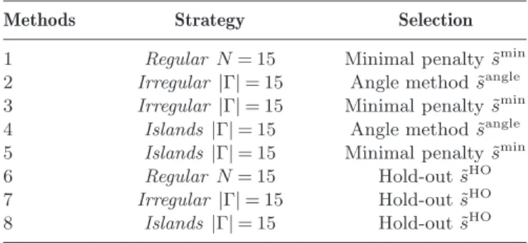
Table 1summarizes our 8 different estimators.
4.2. Simulated design. We have simulated Hawkes processes with param-eters (ν, h), with ν in{0.001, 0.002, 0.003, 0.004, 0.005}, h having a bounded support in (0, 1000] (i.e., A = 1000) and on a sequence of length [−A, T ] with T = 100,000 or T = 500,000. The fact that the process is or not stationary does not seem to influence our procedure with this relatively short memory (indeed T≥ 100A).
The functions h have been designed so that we can see the influence of p (2.1) on the estimation procedure. So f1= 0.004 [200,400] is a piecewise constant nonnegative function on the regular partition Γ (|Γ| = 15) with integral 0.8 and we have tested h = c∗ f1 with c in {0.25, 0.5, 0.75, 1} (i.e., p = 0.2, 0.4, 0.6 and 0.8, respectively). We have also tested a possibly neg-ative function f2 = 0.003 [200,800/3] − 0.003 [2000/3,2200/3] that is piecewise
Table 1
Table of the different methods
Methods Strategy Selection
1 Regular N = 15 Minimal penalty ˜smin
2 Irregular |Γ| = 15 Angle method ˜sangle
3 Irregular |Γ| = 15 Minimal penalty ˜smin
4 Islands |Γ| = 15 Angle method ˜sangle
5 Islands |Γ| = 15 Minimal penalty ˜smin
6 Regular N = 15 Hold-out ˜sHO
7 Irregular |Γ| = 15 Hold-out ˜sHO
constant on Γ. Note that (see Section 2.4) the sign of h should not affect the method (penalized least-square criterion) whereas the log-likelihood may have some problems each time Ψf(·) remains negative on a large interval. The parameter of importance here is the integral of the absolute value, which is here " |f2| = 0.8 and we have tested h = f2. Finally, the method itself should not be affected by a smooth function h: we have used f3 a non-negative continuous function (in fact the mixture of two Gaussian densities) with integral equal to 0.8 and we have tested once again h = f3.
Remark that the mean number of observed points belongs to [125, 12,500] which corresponds to the number of occurrences we could observe in biolog-ical data.
4.3. Implementation. The minimization of γT is actually quite easy since we use a least-square contrast. From a matrix point of view, one can associate to some f in Sm [see (2.9)] a vector of D + 1 =|m| + 1 coordinates
θm= µ aI1 .. . aID ,
where I1, . . . , ID represent the successive intervals of the model m. Let us introduce bm= 1 TN[0,T ] 1 T ! T 0 Ψ(0, I1)(t) dNt .. . 1 T ! T 0 Ψ(0, ID)(t) dNt and Xm= 1 T1!0TΨ(0, I1)(t) dt · · · T1 !T 0 Ψ(0, ID)(t) dt 1 T !T 0 Ψ(0, I1)(t) dt T1 !T 0 Ψ2(0, I1)(t) dt · · · T1 !T 0 Ψ(0, I1)(t)Ψ(0,ID)(t) dt .. . ... . .. ... 1 T !T 0 Ψ(0,ID)(t) dt T1 !T 0 Ψ(0, I1)(t)Ψ(0, ID)(t) dt · · · T1 !T 0 Ψ2(0, ID)(t) dt .
It is not difficult to see that the contrast γT(f ) can be written γT(f ) =−2θmbm+tθmXmθm.
Therefore, the minimizer ˆθm of γT(f ) over f in Sm satisfies Xmˆθm= bm, that is, ˆθm= X−1
despite their randomness, it may be long but not that difficult to compute Xm. It is also possible to compute XΓ and to deduce from it the different Xm’s, when one uses the Islands or Irregular strategies. Nevertheless, both
Islands and Irregular strategies require to calculate each vector ˆθm for the
2|Γ| possible models m and to store them to evaluate the oracle risk (see below). We thus restricted our Monte Carlo simulations to models m with less than 15 intervals. For the analysis of single real data sets, the technical limitation of our programs is |Γ| = 26 due to the 2|Γ| possible models. The programs have been implemented in R and are available upon request.
4.4. Results. The quality of the estimation procedures is measured thanks to two criteria: the risk of the estimators and the associated oracle ratio. • We call Risk of an estimator the Mean Square Error of this estimator over
100 simulations, that is, we compute for each simulation"s − ˆs"2 and next we compute the average over 100 simulations. Note that with the range of our parameters, the error of estimation of ν will be really negligible with respect to the error of estimation for h, so that "s − ˆs"2%"A
0 (h− ˆh)2. • The Oracle Risk is for each method the minimal risk, that is,
minm∈MTRisk (ˆsm). All our methods give an estimator ˜s that is selected
among a family of ˆsm’s. The Oracle Ratio is the ratio of the risk of ˜s divided by the Oracle Risk, that is,
Risk (˜s)
minm∈MTRisk (ˆsm)
.
If the Oracle Ratio is 1, then the risk of ˜s is the one of the best estimator in the family. Note that the definition ofMT and even the definition of ˆsm appearing in the Oracle Ratio may change from one method to another one.
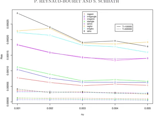
Figure2gives the Risk of our estimators for h = 0.5∗ f1 for various ν and T . We first clearly see that the risk decreases when T increases whatever the method. Then we see that the “best methods” are methods 1, 2 and 4, that is, the Regular strategy with minimal penalty and the Irregular and Islands
strategies with the angle method. For the Irregular and Islands strategies, the
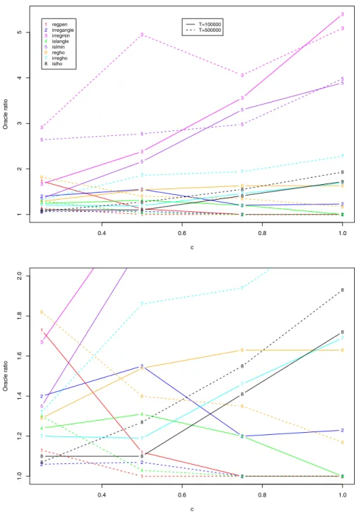
minimal penalty seems to behave like the Hold-out strategies. There seems also to be a slight improvement when ν becomes larger, tending to prove that, if the mean total number of points E(N [0, T ]) = νT/(1− p) grows, the estimation is improved—at least in our range of parameters. Figure3 gives the Oracle Ratio of our estimators in the same context. The Oracle Ratio is really close to 1 for methods 1, 2 and 4 when T = 500,000 whatever ν is. Remark that the Oracle Ratio for the Hold-out estimators (methods 6, 7 and 8) is not that large, but since the estimators ˆsm are computed with half
0.001 0.002 0.003 0.004 0.005 0.00000 0.00005 0.00010 0.00015 0.00020 0.00025 nu Risk 1 1 1 1 1 1 1 1 1 1 2 2 2 2 2 2 2 2 2 2 3 3 3 3 3 3 3 3 3 3 4 4 4 4 4 4 4 4 4 4 5 5 5 5 5 5 5 5 5 5 6 6 6 6 6 6 6 6 6 6 7 7 7 7 7 7 7 7 7 7 8 8 8 8 8 8 8 8 8 8 1 2 3 4 5 6 7 8 regpen irregangle irregmin islangle islmin regho irregho islho T=100000 T=500000
Fig. 2. Risk of the 8 different methods for h = 0.5 ∗ f1 for different values of ν and T .
of the data, their Risks are not as small as the projection estimators used in the penalty methods. This explains why the Risk of the Hold-out methods is large when the Oracle Ratio is close to 1. The Oracle Ratio is improving when T becomes larger for our three favorite methods (namely 1, 2, 4).
Figure 4 gives the variation of the Risk with respect to p (2.1). Since h = c∗ f1 and since c varies, the Rescaled Risk, Risk /c2, gives (up to some negligible term corresponding to ν) the risk of ˜h/c as an estimator of f1. We clearly see that when T or c becomes larger the Rescaled Risk is decreasing. So it definitely seems that if the mean total number of points grows, the estimation is improving. Methods 1, 2 and 4 seem to be still the more precise ones. Figure5gives the Oracle Ratio in the same situation. Once again there is an improvement when T grows at least for our three favorite methods (1, 2 and 4) and the Oracle Ratio is 1 when T = 500,000 and c = 0.8. The same comment about a good Oracle Ratio for the Hold-out methods apply.
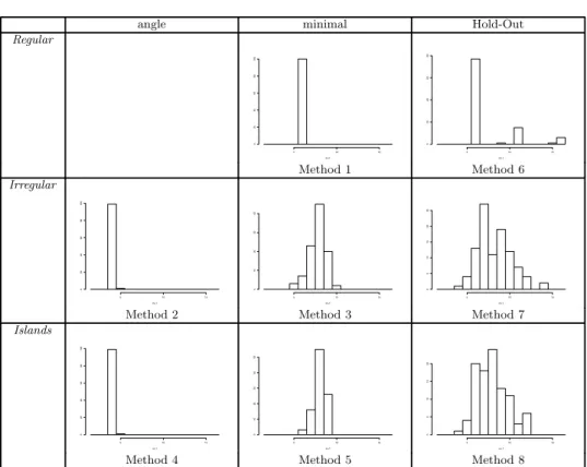
Figure 6 gives the frequency of the chosen dimension, namely | ˆm| + 1 for the different methods. Clearly, methods 1, 2 and 4 are correctly choos-ing the true dimension in most of the simulations when the other methods overestimate the true dimension.
Finally, Figure7 shows the resulting estimators of methods 1, 2 and 4 on one simulation. In particular, before penalizing, note that one clearly sees an angle on the contrast curve at the true dimension and that penalizing
0.001 0.002 0.003 0.004 0.005 12345 nu Oracle ratio 1 1 1 1 1 1 1 1 1 1 2 2 2 2 2 2 2 2 2 2 3 3 3 3 3 3 3 3 3 3 4 4 4 4 4 4 4 4 4 4 5 5 5 5 5 5 5 5 5 5 6 6 6 6 6 6 6 6 6 6 7 7 7 7 7 7 7 7 7 7 8 8 8 8 8 8 8 8 8 8 1 2 3 4 5 6 7 8 1 2 regpen irregangle irregmin islangle islmin regho irregho islho T=100000 T=500000 T=100000 T=500000
Fig. 3. Oracle Ratio of the 8 different methods for h = 0.5 ∗ f1 for different values of ν and T . 0.4 0.6 0.8 1.0 0.0000 0.0005 0.0010 0.0015 0.0020 0.0025 c Risk/c^2 1 1 1 1 1 1 1 1 2 2 2 2 2 2 2 2 3 3 3 3 3 3 3 3 4 4 4 4 4 4 4 4 5 5 5 5 5 5 5 5 6 6 6 6 6 6 6 6 7 7 7 7 7 7 7 7 8 8 8 8 8 8 8 8 1 2 3 4 5 6 7 8 regpen irregangle irregmin islangle islmin regho irregho islho T=100000T=500000
Fig. 4. Rescaled Risk (Risk /c2) of the 8 different methods for h = c ∗ f1 and ν = 0.001, for different values of c and T .
0.4 0.6 0.8 1.0 12345 c Oracle ratio 1 1 1 1 1 1 1 1 2 2 2 2 2 2 2 2 3 3 3 3 3 3 3 3 4 4 4 4 4 4 4 4 5 5 5 5 5 5 5 5 6 6 6 6 6 6 6 6 7 7 7 7 7 7 7 7 8 8 8 8 8 8 8 8 1 2 3 4 5 6 7 8 regpen irregangle irregmin islangle islmin regho irregho islho T=100000 T=500000 0.4 0.6 0.8 1.0 1.0 1.2 1.4 1.6 1.8 2.0 c Oracle ratio 1 1 1 1 1 1 1 1 2 2 2 2 2 2 2 2 3 4 4 4 4 4 4 4 4 5 6 6 6 6 6 6 6 6 7 7 7 7 7 7 7 8 8 8 8 8 8 8 8
Fig. 5. Oracle Ratio of our estimators for h = c ∗ f1 and ν = 0.001 for different values of c and T (top). The bottom picture zooms in on the top picture for Oracle Ratio between 1 and 2.
Fig. 6. Frequency of the chosen dimension | ˆm| + 1 for the different methods when T = 500,000, ν = 0.001 and h = 0.5 ∗ f1. Note that the true dimension is 6 for the Regu-lar method (chosen in 100% of the simulations by method 1) and 4 for the IrreguRegu-lar and Islands methods (chosen in more than 95% of the simulations by methods 2 and 4).
by the angle method (methods 2 and 4) gives an automatic way to find the position of this angle.
Figure8 shows the results for the possibly negative function f2 and only for our three favorite methods (1, 2, 4). For this function only, and because the true dimension is 16 for method 1, we use for method 1, |Γ| = 25. Note that (i) methods 1 and 4 select the right dimension whereas method 2
(Ir-regular strategy) does not see the negative jump and that (ii) it is also more
easy to detect the precise position of the fluctuations on the sparse estimate given by method 4 (compared to method 1). For sake of simplicity, we do not give the Risk values, but it is sufficient to note that, for all the methods, they are small (with a slight advantage for method 4) and that the Oracle
Ratios are close to 1.
Figure 9 gives the same results for the smooth function f3. Of course, since the projection estimators are piecewise constant, they cannot look really close to f3. But in any case, method 1 and more interestingly method
Fig. 7. Contrast (C) and penalized contrast (PC) as a function of the dimension for the
three favorite methods on one simulation with T = 500,000, ν = 0.001 and h = 0.5 ∗ f1.
The chosen estimators (PE) are in blue whereas the function h = 0.5 ∗ f1 is in red.
4 gives the right position for the spikes whereas method 2 does not see the smallest bump.
Finally, let us conclude the simulations by noting that the penalized pro-jection estimators with the Islands strategy and the angle penalty (method 4) seems to be an appropriate method for detecting local spikes and bumps in the function h and even negative jumps.
5. Applications on real data. We have applied the penalized (angle method) estimation procedure with the Island strategy (method 4) to two data sets related to occurrences of genes or DNA motifs along both strands of the complete genome of the bacterium Escherichia coli (T = 9,288,442). In both cases, we used A = 10,000 as the longest dependence between events and the finest partition corresponds to |Γ| = 15.
The first process corresponds to the occurrences of the 4290 genes. Figure
10(top) gives the associated contrast and penalized contrast, together with the chosen estimator of h ( ˆm = 4 and ˆν = 3.64 10−4). The shape of this estimator tells us that:
Fig. 8. Histogram of the selected dimension over 100 simulations (SD). Contrast (C) and penalized contrast (PC) as a function of the dimension for the three favorite methods
on one simulation with T = 500,000, ν = 0.001 and h = f2. The true dimension is 16 for
method 1 (Regular), 6 for method 2 (Irregular) and 3 for method 4 (Islands). The chosen estimators (PE) are in blue whereas the function h = f2 is in red.
• gene occurrences seem to be uncorrelated down to 2600 basepairs, • they are avoided at a short distance (∼0–500 bps) and
• favored at distances ∼700–2000 bps apart.
This general trend has been refined by shortening the support A to 5000 and then to 2000 (see Figure 11). It then clearly appears both a negative effect at distances less than 250 bps, and a positive one around 1000 bps. This is completely coherent with biological observations: genes on the same strand do not usually overlap, they are about 1000 bps long in average, and there are few intergenic regions along bacterial genomes (compact genomes).
Fig. 9. Histogram of the selected dimension over 100 simulations (SD). Contrast (C) and penalized contrast (PC) as a function of the dimension for the three favorite methods
on one simulation with T = 500,000, ν = 0.001 and h = f3. The chosen estimators (PE)
are in blue whereas the function h = f3 is in red.
The second process corresponds to the 1036 occurrences of the DNA motif tataat. Figure 10 (bottom) gives the associated contrast and penalized contrast, together with the chosen estimator of h ( ˆm = 5 and ˆν = 7.82 10−5). The shape of the estimator suggests that:
• occurrences seem to be uncorrelated down to 4000 basepairs, • favored at distances ∼ 0–1500 bps and 3000 bps apart, • highly favored at a short distance apart (less than 600 bps).
After shortening the support A to 5000 (see Figure 11), the shape of the chosen estimator shows that there actually are 3 types of favored distances:
Fig. 10. Contrasts, penalized contrasts and chosen estimators for both E. coli datasets.
very short distances (less than 300 bps), around 1000 bps and around 3500 bps. This trend is again coherent with the fact that (i) the motif tataat is self-overlapping (two successive occurrences can occur at a distance 5 apart), (ii) this motif is part of the most common promoter of E. coli meaning that it should occur in front of the majority of the genes (and these genes seem to be favored at distances around 1000 bps apart from the previous example), (iii) some particular successive genes (operons) can be regulated by the same promoter (this could explain the third bump).
Figure12presents the results of the FADO procedure [12]. Here, we have forced the estimators to be piecewise constant to make the comparison easier. Note, however, that the FADO procedure may be implemented with splines of any fixed degree.
Our results are in agreement with the ones obtained by FADO. Our new approach has two advantages. First, it gives a better idea of the support A of
Fig. 11. Chosen estimators for both E. coli datasets for different values of A: A = 5000 (left, right) and A = 2000 (middle).
Fig. 12. FADO estimators for both E. coli datasets for different values of A: A = 10,000 (left) and A = 2000 (right) for genes or A = 5000 (right) for tataat.
the function h: indeed, the estimator provided by FADO (cf. Figure12 top-left) has some fluctuations until the end of the interval whereas our estimator (cf. Figure 10 top-right) points out that nothing significant happens after 3000 bps. Second, our method leads to models of smaller dimension (|m| = 4 for Islands versus |m| = 15 for FADO). The limitation of our method is essentially that we only consider piecewise constant estimators, but this is enough to get a general trend on favored or avoided distances within a point process.
6. Minimax properties. The theoretical procedures of Proposition1and Theorem1 have more theoretical properties than just an oracle inequality. This section provides their minimax properties. In particular, even if it has not been implemented for technical reasons that were described above, the
Nested strategy leads to an adaptive minimax estimator. Such kinds of
esti-mators were not known in the Hawkes model, as far as we know.
6.1. H¨olderian functions. First, one can prove the following lower bound.
Proposition 3. Let L > 0 and 1≥ a > 0. Let
HL,a={s = (ν, h) ∈ L2/∀x, y ∈ (0, A], |h(x) − h(y)| ≤ L|x − y|a}.
Then
inf ˆ
s s∈Hsup
L,a∩Lη,ρH,P
The infimum over ˆs represents the infimum over all the possible estimators
constructed on the observation on [−A, T ] of a point process (Nt)t. Es
rep-resents the expectation with respect to the stationnary Hawkes process (Nt)
with intensity given by Ψs(·).
But on the other hand, let us consider the clipped projection estimator ¯
sm with m a regular partition of (0, A] such that |m| % (T/ log(T ))1/(2a+1).
If the function h is in HL,a∩ Lη,ρH,P with a∈ (1/2, 1], then, applying Propo-sition1, ¯sm satisfies E("¯sm− s"2)≤ ♦H,P,A,η,ρ,L,a * log(T ) T +2a/(2a+1) .
Compared with the lower bound of the minimax risk (Proposition3), we only lose a logarithmic factor: the clipped projection estimators are minimax on HL,a∩ Lη,ρH,P, with a∈ (1/2, 1], up to some logarithmic term. We cannot go beyond a = 1/2 because one needs|m| .√T in Proposition1.
Of course, we need to know a to find ¯sm, so ¯sm is not adaptive with respect to a. But the clipped penalized projection estimator ¯s with the
Nested strategy can be adaptive with respect to a. It is sufficient to take
J% log2( √
T / log(T )3) to guarantee (3.2). Then we apply Theorem1 with Q = 1.1, for instance. Since #{MT} is of the order log(T ), we obtain that
E("¯s − s")2≤ ♦H,η,P,A,ρ inf m∈MT ( "s − sm"2+ (|m| + 1)log(T ) 2 T ) . If h is inHL,a∩ Lη,ρH,P with a∈ (1/2, 1], then there exists m in MT such that
|m| % (T/ log(T )2)1/(2a+1) and consequently E("¯s− s")2≤ ♦H,η,P,ρ,A,L,a * log(T )2 T +2a/(2a+1) .
Therefore, the clipped penalized projection estimator ¯s with the Nested
strategy and the theoretical penalty given by (3.4) is adaptive minimax on
{HL,a∩ Lη,ρH,P, a∈ (1/2, 1]} up to some logarithmic term.
6.2. Irregular and Islands sets. Let us apply Theorem 1 to the
Irregu-lar strategy and Islands strategy. In both cases, the limiting factor here is
#{MT}. Take N ≤ log2(T ), then #{MT} ≤ T and if Q ≥ 2 we obtain that E("¯s − s")2≤ ♦H,P,A,η,ρ inf
m∈MT ( "s − sm"2+ (|m| + 1) log(T )2 T ) .
To measure performances of those estimators, one needs to introduce a set of sparse functions h, functions that are difficult to estimate with a Nested
strategy. A piecewise function h is usually thought as sparse if the resulting
partition is irregular with few intervals. So we define the Irregular set by SΓ,Dirr := 7
m partition written on Γ, |m|=D Sm. (6.1)
Then, if s belongs to SΓ,Dirr , using the Irregular strategy, the clipped penalized projection estimator satisfies
E("¯s − s")2≤ ♦H,P,η,ρ,ADlog(T ) 2
T .
But for our biological purpose, the sparsity lies in the support of h. So we define the Islands set by
SΓ,Disl := 7 m⊂Γ,|m|=D
Sm. (6.2)
Then, if s belongs to Sisl
Γ,D, using the Islands strategy, the clipped penalized projection estimator also satisfies
E("¯s − s")2≤ ♦H,P,η,ρ,AD
log(T )2
T .
On the other hand it is possible to compute lower bounds for the minimax risk over those sets.
Proposition 4. Let Γ be a partition of (0, A] such that infI∈Γℓ(I)≥ ℓ0.
Let |Γ| = N and let D be a positive integer such that N ≥ 4D. If D ≥
c2(A, η, P, ρ, H) > 1, for c2 some positive constant depending on A, η, P, ρ, H,
then inf ˆ s s∈Sislsup Γ,D∩L η,ρ H,P
Es("s − ˆs"2)≥ ♦H,P,A,η,ρmin* D log(N/D) T , Dℓ0 + and inf ˆ s s∈Sirrsup Γ,D∩L η,ρ H,P Es("s − ˆs"2)≥ ♦H,P,A,η,ρmin * D log(N/D) T , Dℓ0 + .
The infimum over ˆs represents the infimum over all the possible estimators
constructed on the observation on [−A, T ] of a point process (Nt)t. Es
rep-resents the expectation with respect to the stationary Hawkes process (Nt)
To clarify the situation, it is better to take N =|Γ| % log(T ). If D % log(T )a with a < 1 then the lower bound on the minimax risk is of the order log(T )alog log T /T when the risk of the clipped penalized projection estimator (for both strategies) is upper bounded by log(T )a+2/T , and this whatever a is. So our estimator matches the rate 1/T up to a logarithmic term. Of course the most fundamental part is this logarithmic term. Think, however, that there exists some function h in those sets, such that the func-tion belongs to SΓ but to none of the other spaces Sm for m in the family MT described by the Nested strategy. Consequently, a clipped penalized es-timator with the Nested strategy would have an upper bound on the risk of the order log(T )3/T by applying Theorem 1. So the Irregular and Islands strategies have not only good practical properties, but there is also definitely a theoretical improvement in the upper bound of the risk.
7. Technical results.
7.1. Oracle inequality in probability. The following result is actually the one at the origin of Theorem1. Note that this result holds for the practical estimator, ˜s, which is not clipped.
Theorem 2. Let (Nt)t∈R be a Hawkes process with intensity Ψs(·). Let H, η and A be positive known constants such that s = (ν, h) satisfies ν∈ [0, η]
and h(·) ∈ [0, H].
Moreover, assume that the familyMT satisfies
inf m∈MT
inf
I∈mℓ(I)≥ ℓ0> 0.
LetS be a finite vectorial subspace of L2 containing all the piecewise
con-stant functions constructed on the models ofMT. Let R > r > 0 be positive
real numbers, let N be a positive integer and let us consider the following
event:
B = {∀t ∈ [0, T ], N([t − A, t)) ≤ N and ∀f ∈ S, r2"f"2≤ D2T(f )≤ R2"f"2},
where N ([t− A, t)) represents the number of points of the Hawkes process
(Nt)t in the interval [t− A, t). We set Λ = (η + HN )R2/r2 and we consider
ε and x any arbitrary positive constants. If for all m∈ MT pen(m)≥ (1 + ε)3Λ|m| + 1
T (1 + 3 √
2x)2,
then there exists an event Ωx with probability larger than 1− 3#{MT}e−x
such that for all m∈ MT, both following inequalities hold:
εr2
1 + ε"˜s − s" 2
≤ (1 + ε)DT2(sm− s) + (1 + ε−1)DT2(s− s⊥) + r2"s⊥− s"2 (7.1) + r 2 1 + ε"s − sm" 2+ (1 + ε) pen(m) + ♦ ε Λ Tx + ♦ε 1 +N2/ℓ 0 r2T2 x 2,
where s⊥ denotes the orthogonal projection for " · " of s on S, and
r2 ε 1 + εE("˜s − s" 2 B∩Ωx) ≤ * (2 + ε + ε−1)K2+2 + ε 1 + εr 2 + "s − sm"2 (7.2) + (1 + ε) pen(m) + ♦εΛ x T + ♦ε 1 +N2/ℓ0 r2T2 x 2,
where K is a positive constant depending on s such that "f"D≤ K"f" for
all f in L2 (see Lemma 2).
Remark 1. This result is really the most fundamental to understand how the Hawkes process can be easily handled once we only focus on a nice event, namelyB. We have “hidden” in B the fact that the intensity of the process is unbounded: onB, the number of points per interval of length A is controlled, so the intensity is bounded on this event. We have also “hidden” inB the fact that we are working with a natural norm, namely DT, which is random and which may eventually behave badly: on B, DT is equivalent to the deterministic norm" · " for functions in S. More precisely, the result of (7.1) mixes" · " and DT(·) but holds in probability. On the contrary, (7.2) is weaker but more readable since it holds in expectation with only one norm " · ". Note also that B is observable, so if one observes that we are on B, (7.2) shows that a penalty of the type a factor times the dimension can work really well to select the right dimension. Indeed, note that if, in the family MT, there is a “true” model m (meaning that s = sm) and if the penalty is correctly chosen, then (7.2) proves that "˜s − s"2 is of the same order as the lower bound on the minimax risk on m, namely |m|/T (see Proposition
2 for the precise lower bound). In that sense, this is an oracle inequality. The procedure is adaptive because it can select the right model without knowing it. But of course this hides something of importance. If B is not that frequent, then the result is completely useless from a theoretical point of view since one cannot guarantee that the risk of the penalized estimator and even the risk of the projection estimators themselves are small.
Remark 2. In fact, we will see in the next subsection that the choices of N , R, r, MT are really important to control B. In particular, we are not able at the end to manage families of models with a very high complexity as in [5] or in most of the other works in model selection (see Theorem1 and
Section6). This is probably due to a lack of independency and boundedness in the process itself.
Remark 3. Note also that the oracle inequality in probability (7.1) of Theorem2remains true for the more general process defined by (2.14) once we replaceB by B ∩ B' whereB'={∀t ≤ T, λ(t) > 0}. But of course then, B' is not observable. This tends to prove that even in case of self-inhibition a penalty of the type a constant times the dimension is working.
7.2. Control of B. The assumptions of Theorem 1 are in fact a direct consequence of the assumptions needed to controlB, as shown in the follow-ing result.
Proposition 5. Let s∈ Lη,ρH,P and R and r such that
R2> 2 max * 1, η (1− P )2(ηA + (1− P ) −1) + and r2< min* ρ 4, 1− P 8Aη + 1 + . Moreover let N = 6 log(T ) P− log P − 1.
Let us finally assume that S, defined in Theorem 2, is included in SΓ where
Γ is a regular partition of (0, A] such that |Γ| ≤
√ T (log T )3.
Then, under the assumptions of Theorem 2, there exists T0 > 0 depending
on η, ρ, P, A, R and r, such that for all T > T0,
P(Bc)≤ ♦η,P,A 1 T2.
These technical results imply very easily Proposition1and Theorem1. Proof of Theorem 1. We apply (7.2) of Theorem 2 to ˜s. Since ¯s is closer to s than ˜s, the inequality is also true for ¯s. We choose x = Q log(T ) and N , R, r according to Proposition 5. On the complement of B ∩ Ωx, we bound "¯s − s" by η2+ H2A and the probability of the complement of the event by ♦η,P,A,ρ,H* 1 T2 + #{MT} TQ + .
The same control may be applied if T is not large enough. To complete the proof, note finally that K≤ ♦η,P,A. "
Proof of Proposition1. We can apply Theorem2to a family that is reduced to only one model m. If the inequality is true for the nontruncated estimator, and if we know the bounds on s then the inequality is necessarily true for the truncated estimator, which is closer to s than ˜s. Then the penalty is not needed to compute the estimator but it appears nevertheless in both oracle inequalities. We can conclude by similar arguments as Theorem1, but if we take x = log(T ) in (7.2), we lose a logarithmic factor with respect to Proposition1. We actually obtain Proposition1by integrating also in x the oracle inequality in probability (7.1) and we conclude by similar arguments, using that" · "D≤ K" · ". "
8. Sketch of proofs for the technical and minimax results.
8.1. Contrast and norm. First, let us begin with a result that makes clear the link between the classical properties of the Hawkes process (namely the Bartlett spectrum) and the quantity " g2 that is appearing in the definition of the L2 space (2.3).
Lemma 1. Let (Nt)t∈R be a Hawkes process with intensity Ψs(·). Let g
be a function on R+ such that "0+∞g(u) du is finite. Then for all t,
E (*! t −∞ g(t− u) dNu +2) = ν 2 (1− p)2 *! +∞ 0 g(u) du +2 + ! R|Fg(−w)| 2f N(w) dw ≤ ν 2 (1− p)2 *! +∞ 0 g(u) du +2 + ν (1− p)3 ! +∞ 0 g2(u) du, where fN(w) = ν 2π(1− p)|1 − Fh(w)|2
is the spectral density of (Nt)t∈R.
Remark(Notation). Fh is the Fourier transform of h, that is, Fh(x) = "
Re
ixth(t) dt.
Proof of Lemma 1. Let φt(u) = u<tg(t− u). We know (see [8], page 123) that Var (! R φt(u) dNu ) = ! R|Fφ t(w)|2fN(w) dw.
Moreover, since g has a positive support,Fφt(w) = eiwtFg(−w). Hence, Var (! R φt(u) dNu ) = ! R|Fg(−w)| 2f N(w) dw. But we also know that (see [13])
λ = E(λ(t)) = ν 1− p. Consequently, E (*! t −∞ g(t− u) dNu +2) = Var (! R φt(u) dNu ) + * E *! R φt(u) dNu ++2 = Var (! R φt(u) dNu ) + * λ ! +∞ 0 g(u) du +2 , which gives the first part of the lemma. The second part is due to Plancherel’s identity, which states
! R|Fg(−w)| 2dw = 2π! A 0 g2(x) dx, (8.1)
and the fact that fN is upper bounded by ν/[2π(1− p)3] since h is nonneg-ative. "
Lemma1is at the root of Lemma2, which gives the equivalence between the L2-norms, " · " and " · "D, equivalence that is essential for our analysis. Lemma1essentially represents the main feature of the lengthy but necessary computations of Lemma2. The proof of Lemma 2 is consequently omitted and can be found in [23].
Lemma 2. The functional D2T is a quadratic form on L2 and its
expec-tation " · "2
D [see (2.8)] is the square of a norm on L2 satisfying
∀f ∈ L2 L"f" ≤ "f"D≤ K"f", (8.2) where K2= 2 max ( 1, ν (1− p)2 * νA + 1 1− p +) and L2= min( ν 4, 1− p 8Aν + 1 ) . Lemma2 has a direct corollary: γT defines a contrast.
Lemma 3. Let (Nt)t∈R be a Hawkes process with intensity Ψs(·). Then
the functional given by
∀f ∈ L2 γT(f ) =− 2 T ! T 0 Ψf(t) dNt+ 1 T ! T 0 Ψf(t)2dt
Proof. Let us compute E(γT(f )). As λ(t) = Ψs(t), one can write by the martingale properties of dNt− Ψs(t) dt using the associate bilinear form of D2 T(f ) that E(γT(f )) = E ( −2 T ! T 0 Ψf(t) dNt ) + E(DT2(f )) = E ( −2 T ! T 0 Ψf(t)Ψs(t) dt ) +"f"2D ="f − s"2D− "s"2D.
Consequently, E(γT(f )) is minimal when f = s since Lemma 2 proves that " · "D is a norm. "
8.2. Proof of Theorem2. This proof is quite classical in model selection.
It heavily depends on a concentration inequality for χ2-type statistics that has been derived in [20] and which holds for any counting process. The main feature is to use the martingale properties of Nt−
"t
0λ(u) du [see (1.1)]. We do not need any further properties of the Hawkes process to obtain (7.1) (see Remark3).
We give here a sketch of the proof to emphasize that:
1. the oracle inequalities of Theorem 2 hold for ˜s the practical estimator and not only the clipped one, and
2. that (7.1) holds for possible negative function h up to a minor correction (see Remark4 at the end of the proof).
More details may be found in [23].
Proof of Theorem 2. Let m be a fixed partition of MT. By con-struction, we obtain
γT(˜s) + pen( ˆm)≤ γT(ˆsm) + pen(m)≤ γT(sm) + pen(m). (8.3)
Let us denote for all f in L2, νT(f ) = 1 T ! T 0 Ψf(t)(dNt− Ψs(t) dt),
which is linear in f . Then (2.6) becomes γT(f ) = D2T(f−s)−DT2(s)−2νT(f ) and (8.3) leads to
DT2(˜s− s) ≤ DT2(sm− s) + 2νT(˜s− sm) + pen(m)− pen( ˆm). (8.4)
By linearity of νT, νT(˜s−sm) = νT(˜s−smˆ) + νT(smˆ−sm). Now let us control each term in the right-hand side of (8.4).
![Fig. 1. On each line, one can find a model by looking at the collection of red intervals between “[” or “].” For the Nested strategy, here are all the models for J = 3](https://thumb-eu.123doks.com/thumbv2/123doknet/13544060.418841/9.918.200.702.199.549/fig-model-looking-collection-intervals-nested-strategy-models.webp)