HAL Id: hal-02105529
https://hal.archives-ouvertes.fr/hal-02105529
Submitted on 21 Apr 2019
HAL is a multi-disciplinary open access
archive for the deposit and dissemination of
sci-entific research documents, whether they are
pub-lished or not. The documents may come from
teaching and research institutions in France or
abroad, or from public or private research centers.
L’archive ouverte pluridisciplinaire HAL, est
destinée au dépôt et à la diffusion de documents
scientifiques de niveau recherche, publiés ou non,
émanant des établissements d’enseignement et de
recherche français ou étrangers, des laboratoires
publics ou privés.
Joana Oliveira, Mark Wieczorek, Gunther Kletetschka
To cite this version:
Joana Oliveira, Mark Wieczorek, Gunther Kletetschka. Iron Abundances in Lunar Impact Basin Melt
Sheets From Orbital Magnetic Field Data. Journal of Geophysical Research. Planets, Wiley-Blackwell,
2017, 122 (12), pp.2429-2444. �10.1002/2017JE005397�. �hal-02105529�
Iron Abundances in Lunar Impact Basin Melt Sheets
From Orbital Magnetic Field Data
Joana S. Oliveira1,2 , Mark A. Wieczorek3 , and Gunther Kletetschka4,5,6
1Institut de Physique du Globe de Paris, Université Paris Diderot, Paris, France,2CITEUC, Geophysical and Astronomical Observatory, University of Coimbra, Coimbra, Portugal,3Laboratoire Lagrange, Observatoire de la Côte d’Azur, Nice, France, 4Faculty of Science, Charles University in Prague, Prague, Czech Republic,5Institute of Geology, Academy of Science of the Czech Republic, Prague, Czech Republic,6Geophysical Institute, University of Alaska Fairbanks, Fairbanks, AK, USA
Abstract
Magnetic field data acquired from orbit shows that the Moon possesses many magnetic anomalies. Though most of these are not associated with known geologic structures, some are found within large impact basins within the interior peak ring. The primary magnetic carrier in lunar rocks is metallic iron, but indigenous lunar rocks are metal poor and cannot account easily for the observed field strengths. The projectiles that formed the largest impact basins must have contained a significant quantity of metallic iron, and a portion of this iron would have been retained on the Moon’s surface within the impact melt sheet. Here we use orbital magnetic field data to invert for the magnetization within large impact basins using the assumption that the crust is unidirectionally magnetized. We develop a technique based on laboratory thermoremanent magnetization acquisition to quantify the relationship between the strength of the magnetic field at the time the rock cooled and the abundance of metal in the rock. If we assume that the magnetized portion of the impact melt sheet is 1 km thick, we find average abundances of metallic iron ranging from 0.11% to 0.45 wt %, with an uncertainty of a factor of about 3. This abundance is consistent with the metallic iron abundances in sampled lunar impact melts and the abundance of projectile contamination in terrestrial impact melts. These results help constrain the composition of the projectile, the impact process, and the time evolution of the lunar dynamo.1. Introduction
Magnetic field data acquired from orbit show that the Moon possesses many magnetic anomalies that are scattered across its surface (e.g., Hood & Schubert, 1980; Purucker & Nicholas, 2010; Takahashi et al., 2014). The observed anomalies are enigmatic in that the vast majority do not unambiguously correlate with known geologic structures or processes. Nevertheless, it is widely accepted that these anomalies likely are the result of lunar rocks acquiring a thermoremanent magnetization as they cooled in the presence of a long-lived magnetic field (for a review, see Weiss & Tikoo, 2014).
The primary magnetic carrier in lunar rocks is metallic iron (e.g., Fuller & Cisowski, 1987). However, given that most indigenous crustal rocks have very low metal abundances, they cannot easily account for the magni-tudes of the observed magnetic anomalies (Wieczorek et al., 2012). Mare basalts typically contain less than 0.1 wt % metallic iron, and pristine anorthositic materials contain even less (e.g., Brecher et al., 1974; Pearce et al., 1973, 1974). In contrast, lunar impact melt breccias derived from the largest basins often contain elevated abundances of metallic iron (1–2 wt %), and this iron is believed to be derived from the projectile that formed the basin (e.g., Korotev, 2000). Terrestrial impact melt rocks often contain traces of the projectile as well, with projectile abundances in the melt sheet ranging from less than 1 wt % to up to several weight percent (Tagle & Hecht, 2006; Tagle et al., 2009). We thus suspect that some lunar magnetic anomalies are a result of exogenic metallic iron that was delivered to the Moon by asteroidal projectiles.
Though many of the strongest lunar magnetic anomalies are not associated with known geologic processes, such as the prominent anomaly centered on the Reiner gamma swirl albedo feature on the nearside hemi-sphere (e.g., Hemingway & Garrick-Bethell, 2012), a few are in fact associated with large impact basins (e.g., Halekas et al., 2003; Hood, 2011; Le Bars et al., 2011). Based on the most recent global magnetic field models that make use of both Lunar Prospector and Kaguya data (Tsunakawa et al., 2015), basins with unam-biguous magnetic signatures include Serenitatis, Nectaris, Crisium, Mendel-Rydberg, and Humboldtianum.
RESEARCH ARTICLE
10.1002/2017JE005397
Key Points:
• Some Nectarian-aged lunar impact basins possess magnetic anomalies where an impact melt sheet is expected
• Small quantities of projectile-derived metallic iron are sufficient to explain the observations
Correspondence to: J. S. Oliveira,
Citation:
Oliveira, J. S., Wieczorek, M. A., & Kletetschka, G. (2017). Iron abundances in lunar impact basin melt sheets from orbital mag-netic field data. Journal of Geophysical
Research: Planets, 122, 2429–2444.
https://doi.org/10.1002/2017JE005397
Received 19 JUL 2017 Accepted 3 NOV 2017
Accepted article online 20 NOV 2017 Published online 4 DEC 2017
©2017. American Geophysical Union. All Rights Reserved.
The associated magnetic anomalies are generally in the center of the basin, interior to the peak ring (Neumann et al., 2015), where the thickest portion of the impact melt sheet is predicted to be found (e.g., Cintala & Grieve, 1998). Some of the best preserved basins possess an inner depression just interior of the peak ring (Neumann et al., 2015), and this feature has been suggested to be a result of thermal contraction of a thick melt sheet (Vaughan et al., 2013). When such a feature is present, the magnetic signature is generally located within the inner depression, implying that it is the impact melt that is the source of magnetization.
As another example, Wieczorek et al. (2012) noted that the largest concentration of magnetic anomalies on the Moon is located on the northern rim of the giant South Pole-Aitken impact basin that is located on the Moon’s farside hemisphere. Using a numerical hydrocode, they showed that if this basin formed by a mod-erately oblique impact, with the projectile traveling from the south to north (Garrick-Bethell & Zuber, 2009), a significant quantity of projectile materials would have been deposited on the downrange (i.e., northern) rim, precisely where the magnetic anomalies are found. As asteroidal materials can contain large quantities of metallic iron (either from the core of a differentiated object or from undifferentiated chondritic materials), this iron-rich material could have become magnetized if it cooled in the presence of a global magnetic field. Since chondritic materials often contain orders of magnitude more metallic iron than pristine indige-nous lunar crustal rocks, integrated thicknesses of only tens to hundreds of meters of projectile materials are required to account for the observed magnetic field strengths.
An alternative explanation for the strong magnetic anomalies on the farside hemisphere of the Moon is that they are the result of ejecta deposited near the antipodes of the largest nearside basins. The strongest of these anomalies are approximately antipodal to the Imbrium, Serentitatis, Crisium, and Orientale basins (e.g., Hood et al., 2001; Mitchell et al., 2008). As a result of the spherical geometry of the Moon, it has been shown that under favorable conditions, impact ejecta deposits would increase in thickness as one approached the point antipodal to the impact point (Haskin, 1998; Hood & Artemieva, 2008; Wieczorek & Zuber, 2001). It has been also shown that the expansion of an impact generated plasma cloud could amplify ambient mag-netic field strengths near the basin antipode and subsequently magnetize these deposits (Hood & Artemieva, 2008; Hood & Huang, 1991). Regardless, in order to account for the large observed magnetic field strengths, the impact ejecta would likely need to contain higher than average concentrations of metallic iron, and the most natural source of such iron would be metal derived from the projectile that formed these basins. In this study, we estimate the abundance of metallic iron within impact basin melt sheets by inverting for the magnetization in lunar impact basins. The abundance of iron metal is then derived from a relationship based on laboratory experiments. We first describe in section 2.1 how we estimate the average magnetization of the basin melt sheet using the unidirectional magnetization model of Parker (1991), and in section 2.2 we develop a technique that relates the abundance of metallic iron to the magnetizing field strength, magnetization, and rock magnetic properties. Next, in section 3, using the Mendel-Rydberg basin as an example, we describe how we compute the average magnetization from orbital data and derive the metallic iron abundance. We then apply this approach to four more large basins that contain a central magnetic anomaly. In section 4, we com-pare our results with both lunar samples and terrestrial impact melt rocks. We then discuss some implications that these results have for magnetic anomalies not only on the Moon but on the other planets as well. Finally, we conclude by discussing how our results may help in constraining the composition of projectile, the impact process, and the time evolution of the lunar dynamo.
2. Iron Abundances From Orbital Magnetic Field Data
We devise a technique where orbital magnetic field data can be used to determine the abundance of metallic iron in large impact basins. In the first subsection, we describe how the unidirectional magnetization model of Parker (1991) can be used to invert orbital magnetic field data for the moments of isolated dipoles. Using a priori assumptions on the thickness and geometry of the source, we then convert the dipole moments into an average magnetization. In the following subsection, we describe a model that relates the magnetization to the abundance of magnetic carriers and the strength of the magnetizing field. Though this technique is tailored to the Moon, where metallic iron is the primary magnetic carrier, in principle, it could be generalized to other planets if the magnetic carrier were known a priori.
2.1. Impact Basin Magnetization From Orbital Magnetic Field Data
We make use of a method developed by Parker (1991) to estimate equivalent dipole moment strengths from orbital magnetic field data. This method was first used to determine the direction of magnetization of
terrestrial seamounts (Parker, 1991), and more recently, this method was adapted to determining the direc-tion of magnetizadirec-tion of isolated crustal magnetic anomalies on the Moon (Oliveira & Wieczorek, 2017). In contrast to these previous studies that used Parker’s method to determine paleopole positions, here we focus on the spatial distribution of dipole moment strengths.
In this model, continuous magnetization within the crust is discretized using unidirectional equivalent source dipoles, whose equivalent magnetic moment varies with position. The assumption of unidirectional magne-tization is here justifiable given that the direction of magnemagne-tization from a core-generated magnetic field is unlikely to change substantially during the time it takes an impact melt sheet to cool below the blocking temperature of iron. In particular, the upper 1 km and 5 km of the melt sheet should cool below the blocking temperature of iron in about 10,000 years and 1 million years, respectively (Le Bars et al., 2011). By assuming unidirectional magnetization, Parker (1991) showed that a volumetric distribution of magnetization is equiv-alent to unidirectional dipoles placed on the surface in the limit where the cell size approaches 0. With dipoles residing solely on the surface, the dimensionality of the problem is considerably reduced, and the magneti-zation can be described as
M(si) = ̂m m(si), m(si)≥ 0 , (1) where ̂m is the unit direction of magnetization, and m(si) is the dipole moment at vectorial position si. As explained by Oliveira and Wieczorek (2017), for the lunar case where there is no main dipolar magnetic field, instead of analyzing the component that is aligned with the global field as was done in Parker’s initial study, we analyze only the radial magnetic field component. The magnetic field d in the radial direction̂r at observation point j is calculated as the sum of the contributions from the dipoles located at position si
dj= Nd ∑
i=1
gj(si) m(si), j = 1, … , Nobs, (2)
where the contribution of a single dipole at location i is given by the kernel
gj(si) = 𝜇0 4𝜋 (3̂m ⋅ (r j− si)̂rj⋅ (rj− si) |rj− si|5 − ̂m ⋅ ̂rj |rj− si|3 ) . (3)
Nobsand Ndcorrespond to the number of observations and the number of dipoles in the crust, and rjand si are the vector positions of the observations and dipoles relative to a fixed planetocentric origin, respectively. These equations may be written in the matrix form as
d = G(̂m) m, (4)
where d is a vector of the magnetic field observations projected in the direction̂rj, the matrix G depends upon the assumed direction of magnetization ̂m and contains the elements given by equation (3), and m is a vector that contains the positive magnitudes of the surface dipoles at locations si.
As all elements in the vector m are positive, equation (4) can be solved using the technique of nonnegative least squares analysis (Lawson & Hanson, 1974). For each magnetization direction ̂m, the locations of the surface dipoles that best fit the data, the surface dipole intensities, and the root-mean-square (RMS) misfit between the model and observations are determined. The best magnetization model corresponds to the minimum RMS misfit obtained from the set of all magnetization directions. A property of the nonnegative least squares solution is that the number of nonzero dipoles on the surface is always less than or equal to the number of observations, Nobs. Thus, in practice, we place many more dipoles on the surface than there
are observations and let the algorithm choose naturally those positions that best fit the data. As discussed in Oliveira and Wieczorek (2017), strong magnetic fields can sometimes be predicted to occur just outside of the domain that is being modeled. To counter these edge effects, we place the surface dipoles in a circle of radius rd, and compare the predictions with the model in a slightly larger circle of radius robs. As the spacecraft
observations were made about 30 km above the surface, robsneeds to be about 30 km larger than rd. Our inversion provides the dipole moments of a set of individual dipoles placed on the surface. We next need to convert this into a volumetric magnetization, which we do by assuming the thickness and geometry of the central impact melt sheet. Based on numerical simulations, the thickest portions of a basin’s impact melt
sheet are thought to lie interior to the peak ring (e.g., Cintala & Grieve, 1998). The peak ring has a diameter that is about half of the diameter of the basin (Baker et al., 2011), and for the best preserved basins, an inner topographic depression is often present just interior to the peak ring (see Neumann et al., 2015). The inner depression is thought to be the thickest portion of the impact melt sheet that subsequently cooled and sub-sided (Vaughan et al., 2013). By assuming a thickness of the melt sheet, the average magnetization of the melt sheet is estimated by dividing the sum of the nonzero dipole intensities within the inner depression by the melt sheet volume. As discussed further in section 3.1, we will use a value of 1 km for the thickness of the magnetized zone of the melt sheet.
2.2. Estimation of Metallic Iron Abundances From Magnetization
At the present time, the Moon has no magnetic fields generated by a core dynamo and the magnetic anoma-lies observed from orbit are a result of remanent magnetization within the crust. This magnetization likely represents a thermoremanent magnetization that was acquired in an ancient, now extinct, core field, when crustal rocks cooled through their magnetic blocking temperatures (e.g., Weiss & Tikoo, 2014). The dominant magnetic carrier of lunar rocks is known to be metallic iron that is alloyed with small quantities of nickel (e.g., Fuller & Cisowski, 1987), and whose Curie temperature is 1038 K (Dunlop & Özdemir, 2015). In this section, we develop a technique for estimating the abundance of metallic iron in the crust when only the crustal magnetization is known.
If crustal rocks were available for analysis in the laboratory, the volumetric concentration of the magnetic carrier c could be obtained from the ratio of the measured saturation magnetization of the rock Msto the saturation magnetization of the dominant magnetic carrier, which is here assumed to be metallic iron
c = Ms MFe
s
. (5)
Though MFe
s is a known constant of 1.715 × 10⁶ A m−1 (e.g., Dunlop & Özdemir, 2015), the saturation magnetization of the rock is not.
We estimate the rock’s saturation magnetization by making use of two relations. The first is the squareness
sof the hysteresis loop, which is the ratio of the saturation remanent magnetization Mrsto the saturation magnetization:
s = Mrs
Ms. (6)
It will be shown below that this parameter varies only by a factor of about 2 for a wide range of lunar rocks. The second is an empirical relationship between the acquired thermoremanent magnetization of a rock and the applied magnetic field B. We use the standard empirical approach developed by Gattacceca and Rochette (2004) that is based on numerous thermoremanent magnetization acquisition experiments on lunar, terrestrial, and synthetic samples. In this method, the ratio of the thermoremanent magnetization of a rock
Mtrto the saturation remanent magnetization Mrsis proportional to the applied magnetic field as given by
B = aMtr Mrs
. (7)
For rocks containing common magnetic minerals, the empirical scaling constant is found to be approximately independent of the magnetic carrier and the carrier’s domain state. The constant a has a value of about 3,000 μT with a multiplicative uncertainty of a factor of 2. A recent tabulation in Weiss and Tikoo (2014) of experiments that calibrate this technique arrive at a concordant value. Replacing Msin equation (5) by the relation from equation (6) and then replacing Mrsby that from equation (7) yields
c = a s B Mtr MFe s . (8)
This equation allows to estimate the volumetric concentration of the magnetic phase from the rock mag-netization, the saturation magnetization of the magnetic species, the rock squareness, and the magnetizing field strength.
Table 1
Squarenesss = Mrs∕Msof Apollo Samples
Lithology s 𝜎⋆ N Sources
Mare basalts 0.0064 1.6 34 Fuller and Cisowski (1987), Rochette et al. (2010), and Cournède et al. (2012)
Norites 0.0031 1.6 3 Fuller and Cisowski (1987) and Cournède et al. (2012)
Anorthosites 0.0056 – 2 Fuller and Cisowski (1987)
Mafic impact melt breccias 0.0050 2.2 15 Fuller and Cisowski (1987) (excluding 60225) and Cournède et al. (2012)
Note.Nis the number of samples used to calculate the median of a lognormal distribution, and𝜎⋆is the multiplicative uncertainty.
We note that a slightly different scaling approach has been developed by Kletetschka et al. (2004) (see also Kletetschka & Wieczorek, 2017) that is based on thermoremanent magnetization acquisition experiments for individual magnetic species. This approach accounts for the differing saturation magnetizations of the minerals and can successfully account for the discrepant behavior of hematite when using the approach of Gattacceca and Rochette (2004). For the case of metallic iron, the scaling constant is predicted to be 3 times larger than that of the relation of Gattacceca and Rochette (2004). If this relation were used to obtain the pale-ointensity from isothermal saturation remanent magnetization experiments, the field strength would thus be 3 times larger. Nevertheless, as equation (8) involves the ratio of the scaling constant and magnetizing field strength, these two factors cancel and the concentration of the magnetic mineral would not be changed. In this study we will use equation (7) but acknowledge that the technique of Kletetschka et al. (2004) might be better equipped when investigating individual mineral species.
When working with inferred magnetizations from analyses of orbital magnetic field data, the squareness ratio of the magnetized rocks in the crust is, in general, not known. Nevertheless, for lunar crustal rocks, where iron is predominantly in the multidomain state (e.g., Fuller & Cisowski, 1987), this value is relatively well constrained. The squareness ratio of lunar rocks can be found in several publications, and using these values, we calculate the average squareness for the major rock types of mare basalts, plutonic norites, plutonic anorthosites, and mafic impact melt breccias. We make the assumption that the individual values are lognor-mally distributed, and in Table 1 we provide the exponential of the average value of the logarithms of these values (which is approximately the median of the data) and provided the value of𝜎⋆which corresponds to the 1 −𝜎 multiplicative uncertainty of the lognormally distributed data (e.g., Limpert et al., 2001). We make use of the data in Table 3 of Fuller and Cisowski (1987), and using the original sources, we correct typos for entries of the mare basalts 10024,22 and 74275,56 and the mafic impact melt breccia 60315,47. We included the measurements of the mare basalt samples 14053, 15555, 15556, and 70215 from Rochette et al. (2010), as well as the lunar samples in Cournède et al. (2012). Lastly, we neglect the “glassy melt” 60255 in Fuller and Cisowski (1987) that is atypical by about a factor of 10 with respect to the other impact melt breccias and which was not included in the selection of impact melt breccias used in the study of Wieczorek et al. (2012). The values of s are found to be comparable for the mare basalts, norites, anorthosites, and mafic impact melt breccias, with averages of 0.0064, 0.0031, 0.0056, and 0.0052, respectively. The mare basalts, norites, and mafic impact melt breccias have respective multiplicative uncertainties of 1.6, 1.6, and 2.2, whereas the small number of anorthosite samples precludes calculating an uncertainty. If the sample 60255 were included with the impact melt breccias, the squareness would increase slightly from 0.0050 to 0.0058. Given that this study will be concerned with magnetic anomalies found in the centers of large impact basins, and that a metal-rich impact melt sheet is the likely source of these anomalies, we will make use only of the squareness for the mafic impact melt breccias.
Using the numerical values of s, a, and MFe
s , equation (8) can be written as
c = 3.5 × 10⁻⁷Mtr
B . (9)
The weight percent of metallic iron is estimated from the relation
wt % Fe metal = c𝜌Fe
Figure 1. Magnetic field intensity at 30 km altitude from the model of Tsunakawa et al. (2015). White circles correspond
to the main rim diameter of those basins associated with central magnetic anomalies. For reference, the red stars denote the landing sites of Apollo missions. The map is presented in a global Molleweide projection centered at 0∘E, and grid lines are shown every 30∘of latitude and longitude.
where the density of metallic iron𝜌Feis taken to be 7,600 kg m−3and the density of the silicates𝜌sis assumed to be 3,000 kg m−3. Finally, based on paleomagnetic analyses, we will assume that the strength of the
core-generated field was 72 μT when the large impact basins formed, which is the average value from samples with ages between 4.25 and 3.56 Ga (see Weiss & Tikoo, 2014). Nevertheless, it is noted that this paleointensity is uncertain by about a factor of 1.7 as the paleointensity measurements vary between about 42 and 111 μT during this time interval.
3. Analysis of Magnetic Anomalies Within Large Basins
We have made use of the global magnetic field model of Tsunakawa et al. (2015) to investigate 21 large impact basins that have been identified in previous studies as having potentially central magnetic anomalies (Halekas et al., 2003; Hood, 2011; Hood & Spudis, 2016; Le Bars et al., 2011). Though many of these basins do have mag-netic anomalies, the anomalies are often not isolated and merge with regional clusters of anomalies that are probably unrelated to the basin. For some specific basins where the magnetic anomaly is weak, such as the Schrödinger and Imbrium basins as investigated by Hood and Spudis (2016), we found no magnetic signal in the Tsunakawa et al. (2015) global field model. From our survey, only five basins have magnetic anomalies in their interiors that are clearly related to the basin forming process: Mendel-Rydberg, Humboldtianum, Nectaris, Serenitatis, and Crisium basins. In this section, we first describe the principal inversion steps for the basins in our study. We then describe in detail the results for the Mendel-Rydberg basin, which is an unam-biguous example of a basin with a central magnetic anomaly. Following this, we present the results for the other four basins of our study. Figure 1 shows the locations of the basins analyzed in this study superposed on the magnetic field strength map of Tsunakawa et al. (2015).
3.1. Model Description
We follow the same modeling procedures as in Oliveira and Wieczorek (2017). We use the radial component of the magnetic field model of Tsunakawa et al. (2015) that possesses a 0.5∘ spatial resolution at 30 km altitude and which is based on Lunar Prospector and Kaguya vector magnetic field measurements. The radial compo-nent contains all the information required to derive the other two orthogonal compocompo-nents of the magnetic field (see Tsunakawa et al., 2014), so using this single component is sufficient for our inversions. A grid of equally spaced dipoles (Katanforoush & Shahshahani, 2003) is placed at the lunar surface with a 0.4∘ resolution at the equator, centered over the magnetic anomaly within a circle of radius rd. Magnetic field observa-tions used in calculating the misfit between the model are retained in a slightly larger circle of radius robs. In order to avoid edge effect issues during the inversion, the radius of the circle that contains the data is taken to be 1∘ larger than the circle that outlines the distribution of equivalent source dipoles (see Oliveira & Wieczorek, 2017).
In our inversions, the number of dipoles placed on the surface Ndis greater than the number of observa-tions Nobs. Nevertheless, as a result of the properties of the nonnegative least squares inversion, only less than
Nobsdipoles will have nonzero values. For small basins, the circle that encompasses the observations is
cen-tered over the basin with the same radius of the basin’s main ring. For reasons of computational tractability, it was necessary to choose the radius of robsto be smaller than the basin rim diameter for the larger basins.
This, however, should not affect our results as the magnetic anomalies of interest lie within the smaller peak ring that is well sampled. Furthermore, for some basins, robswas chosen to be smaller than the basin rim to exclude regional magnetic anomalies that do not have a clear genetic relation to the basin.
We perform the nonnegative least squares inversion in order to determine the dipole locations and their dipole moments, as well as the RMS misfit between the modeled field and observations. This is repeatedly per-formed for each magnetization direction, over all directions using a planetocentric unit vector that is varied over a 4∘ equidistant grid of polar and azimuth angles. Using the nonzero dipole moments, we next calculate the average magnetization within the inner depression of the basin using the coordinates and diameters from Neumann et al. (2015). This is done simply by dividing the sum of these dipole moments by the source volume. Noting that all basins in our study are Nectarian in age (i.e., older than about 4 Ga), we assume a representa-tive surface field strength of 72 μT as discussed in section 2.2. Finally, we use the derived magnetization along with the assumed surface field strength to determine the concentration of metallic iron using equation (9). Perhaps the biggest source of systematic bias in our study is the assumed thickness of the impact melt sheet. The total amount of melt generated during a hypervelocity impact is highly dependent upon not only the impact velocity but also the initial temperature profile of the crust and mantle (e.g., Pierazzo et al., 1997). In a study by Potter et al. (2013), the amount of melt generated during the formation of the 937 km diameter Orientale basin was investigated. Partial melting (as opposed to total fusion) was modeled, and two possible initial temperature profiles were considered. Assuming that all impact melt derived from the mantle ended up within the inner depression, the thickness of the melt sheet is predicted to be 12 and 26 km for their two tem-perature profiles, respectively. These thicknesses, however, do not consider that some melt from the mantle would be excavated or displaced outside of the transient cavity (e.g., Miljkovi´c et al., 2015) nor that not all melt within the extensive partial melt zone would be extracted and accumulate at the surface. These thicknesses should thus be considered as upper limits. Even if the impact melt sheet thickness were known, it is likely that any metallic iron present would sink toward the bottom of the pool as a result of its higher density with respect to the silicate melt (e.g., Rubie et al., 2003). The region of the melt sheet that is magnetized might thus correspond to a considerably thinner layer than the total melt sheet thickness. Given all these uncertainties that are difficult to model, and for the sake of simplicity, we will assume that the magnetized portion of the impact melt sheet corresponds to a layer that is 1 km thick. If the magnetized zone were thicker than this, the average magnetization would decrease proportionally.
It is difficult to assign a robust uncertainty to our metallic iron abundances, as there are several sources of error and bias in our analysis. The variance associated with the squareness of lunar rocks implies an uncertainty of a factor of about 2.2. The magnetic field strength from isothermal paleomagnetic studies has a spread of values encompassing a factor of 1.7 (Gattacceca & Rochette, 2004; Weiss & Tikoo, 2014). There is also a factor of 2 variation in magnetic field strength between the pole and equator for a dipolar field, which is difficult to quantify for a given basin as significant true polar wander might have occurred (e.g., Takahashi et al., 2014) or the dipole might not always have been aligned with the rotation axis Oliveira and Wieczorek (2017). We find it unlikely that all of these uncertainties would conspire to either overestimate or underestimate the metal abundances by the maximum factor of about 7. Assuming that the error sources are independent and adding these factors in quadrature provides a factor of 3.4. In addition to this error, one must also consider the systematic bias associated with our assumed thickness of the magnetized zone in the melt sheet.
3.2. Mendel-Rydberg Basin
We demonstrate our approach for the Mendel-Rydberg basin that has an unambiguous magnetic anomaly that is located precisely in the center of the basin. As shown in Figure 2 (top left), Mendel-Rydberg is one of the largest lunar basins. In this topographic map, three ring structures are highlighted: the main crater rim with a diameter of 650 km, a probable peak ring with a diameter of 325 km, and an inner depression with a diameter of 203 km (diameters from Neumann et al., 2015). The magnetic field intensity at 30 km altitude is plotted in Figure 2 (top middle), and comparing this to the basin’s topographic ring structure, it is seen that
Figure 2. (top row) (left) Topography, (middle) observed magnetic field strength at 30 km altitude, and (right)
the magnetic moments of the retained dipoles in the inversion for the Mendel-Rydberg basin. (bottom row) (left) Observed radial magnetic field, (middle) the best fit model radial magnetic field, and (right) the difference between the observations and model. Black circles delimit the basin main rim (solid line), peak ring (dash-dotted line), and inner depression (dashed line) using the diameters of Neumann et al. (2015). Blue circles delimit the grid of observations (solid line) and dipoles (dashed line). The locations of the data points and dipoles used in the inversion are denoted by dots in Figure 2 bottom left and bottom middle, respectively. Images are presented using a Lambert azimuthal equal-area projection with grid lines spaced every 10∘of latitude and longitude.
the magnetic anomaly is almost entirely confined to within the inner depression. The magnetic anomaly is not perfectly centered within the inner depression but is seen to be displaced slightly to the southwest. In Figure 2 (bottom row), we show the radial magnetic field data used in our inversions (left), the best fitting radial magnetic field (middle), and the difference between the two (right). In addition to plotting the basin ring diameters in these images, we also plot the diameters of the circles robsand rdin blue that delineate the regions where the misfit was calculated and where the surface dipoles were placed, the locations of the observations (Figure 2, bottom left), and the locations of the dipoles placed on the surface (Figure 2, bottom middle). As is shown in Figure 2 (bottom right), our method retrieves well the radial magnetic field with an RMS misfit of 0.21 nT, which is low in comparison to the strength of the central anomaly. As an additional detail, we note that the paleopole position for this anomaly is located at the geographical equator (48∘W, 2.4∘N), consistent with the results of Oliveira and Wieczorek (2017) showing that several magnetic anomalies have equatorial paleopoles.
The locations of the nonzero dipoles and their dipole moments are shown in Figure 2 (top right). As is easily seen, the vast majority of the dipoles have zero moments, and the strongest moments correspond to where the observed magnetic field is the largest (see Table 2). Almost all of the strongest dipoles are found within
Table 2
Location (Lat, Lon), Basin Diameter, Angle With Respect to Local North (𝛼), Distance (d) Between Centroid of the Inner Depression and the Main Rim, the RMS Misfit of the Best Fitting Model, the Average Magnetization in the Basin’s Inner Depression (M) and the Corresponding Volumetric Concentration (c) and Weight Percent of Metallic Iron in the Melt Sheet
Basin Lat (deg) Lon (deg) Diameter (km) 𝛼(deg) d(km) Misfit (nT) M(A m−1) c(vol %) wt % Fe metal
Humboldtianum 57.3 82 .0 618 35 19.7 0.16 0.10 0.049 0.12
Mendel-Rydberg −49.8 265.4 650 215 14.0 0.21 0.37 0.18 0.45
Nectaris −15.6 35.1 885 279 33.2 0.24 0.09 0.044 0.11
Serenitatis 25.4 18.8 923 197 40.3 0.17 0.14 0.067 0.17
Crisium 16.8 58.4 1076 252 34.7 0.33 0.33 0.16 0.41
Note. The Average Magnetization in the basin’s inner depression is calculated assuming 1km thick impact melt deposit.
the basin’s inner depression. Only a few strong dipoles are located exterior to the inner depression, and most of these are located near the edge of the modeling domain and could represent artifacts with how the edge of the modeling domain was treated. In comparing the distribution of dipole moments with the magnetic field observations, we note that the strong dipoles are more concentrated within the inner depression than the magnetic field is.
We calculate the total dipole moment of the dipoles in the inner depression to be 1.18 × 10¹³A m2. Using
203 km as the diameter of this depression, along with an assumed 1 km thickness for the melt sheet, we cal-culate the average magnetization of the melt sheet to be 0.37 A m−1. Making use of equation (9) and a surface
field strength of 72 μT, the average volumetric concentration of metallic iron in the melt sheet is 0.18%. Taking into account the difference in density between iron and silicates, the average weight percentage of metallic iron in the inner depression for Mendel-Rydberg is 0.45 wt. %. It should be noted that the magnetization within the melt sheet varies by a factor of about 4, so that significant variations in the abundance of metallic iron should be expected.
3.3. Impact Melt Sheet Iron Abundances
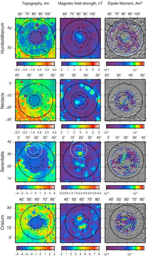
Figure 3 shows the inversion results for the other basins in our study: Humboldtianum, Nectaris, Serenitatis, and Crisium. Figure 3 (left column) plots the topography of the basin, Figure 3 (middle column) plots the observed magnetic field strength, and Figure 3 (right column) plots the intensity of the magnetic moments of the best fitting dipoles on the surface. We summarize the inversion results for both these basins and Mendel-Rydberg in Table 2, which includes the basin size and location, the RMS misfit, the average magneti-zation within the inner depression, and the average abundance of metallic iron in the inner depression. From the basins studied in this work, only Mendel-Rydberg has an unambiguous inner depression in its center. Topography and GRAIL Bouguer gravity data nevertheless reveal that the Nectaris and Crisium basins have a probable inner depression and that Humboldtianum and Serenitatis have a possible inner depression. The uncertainty in the identification of the inner depression (as well as its diameter) is due to a poor preser-vation or/and development of the structure and partial burial by the younger mare basalt that flooded the interiors of these basins. Regardless, Neumann et al. (2015) provide approximate diameters for the inner depression, which are always smaller than the associated peak ring structure.
For each of these basins we find at least one coherent magnetic anomaly within the basin inner ring. When there are multiple magnetic anomalies in the basin center, they are always located within the inner rings. For Humboldtianum, a single elongated magnetic anomaly is located within the inner depression with an amplitude of about 1.7 nT. For Nectaris, a single magnetic anomaly of amplitude 2.2 nT is located in the inner depression. Somewhat stronger anomalies of about 3.3 nT are located at greater distances from the basin center near the main crater rim, but it is not obvious if these anomalies are genetically related to the basin itself. We note that the region where the crust was excavated and thinned during the impact event is largely con-fined to within the peak ring (Neumann et al., 2015), and anomalies that are located outside of this structure could represent preexisting magnetized materials. For the Serenitatis basin, two weak anomalies with magni-tudes of about 1.5 nT are located within the southern portion of the inner depression, and a slightly stronger anomaly of 2.6 nT is located just north of the inner depression. The Serenitatis impact structure could be the result of two overlapping basins (e.g., Neumann et al., 2015) or a single oblique impact. For this study, we treat
Figure 3. (left column) Topography, (middle column) observed magnetic field strength, and (right column) the magnetic
moments of the retained dipoles in the inversion for the Humboldtianum, Nectaris, Serenitatis, and Crisium impact basins. Black circles delimit the basin main rim (solid line), peak ring (dash-dotted line), and inner depression (dashed line) using the diameters of Neumann et al. (2015). Gray circles delimit the main ring (solid line) and the inner ring (dashed line) for the Serenitatis North basin. Blue dashed circles delimit the region where dipoles are placed on the surface, and for reference, red stars denote the Apollo landing sites. Images are presented using a Lambert azimuthal equal-area projection with grid lines spaced every 10∘of latitude and longitude.
it as a single impact structure, but we note that the northern magnetic anomaly could perhaps be related to a smaller superposed impact basin. Finally, the Crisium impact basin possesses two strong isolated magnetic anomalies that are confined to the basin’s inner depression. The two anomalies in Crisium with magnitudes of 7.6 and 5.1 nT are the largest in our study.
For all basins, the RMS misfits obtained in the inversions are lower than 0.33 nT, which is well below the magni-tude of the central magnetic anomalies. In general, the locations of the strongest dipoles in our inversions are highly correlated with the strength of the magnetic field, as is to be expected when the altitude of observation is small compared with the size of the structure. For Humboldtianum and Nectaris, the strongest anomalies are almost entirely located with the inner depression. For Crisium, the strong anomalies are largely confined to the inner depression, with a few being located between the inner depression and peak ring. For Serenitatis, however, the strongest anomalies are found to lie in a single elongated structure within the inner depression, even though the magnetic intensity is composed of three isolated structures. A portion of this structure extends beyond the inner depression in the northern portion of the basin but is entirely confined to within the peak ring structure.
For each of these basins, we calculated the total dipole moment, as well as the average implied magnetization within the inner depression, just as was done for the Mendel-Rydberg basin in the preceding subsection. We find that the Humboldtianum and Nectaris basins are the two basins with the lowest metallic iron content of 0.12 wt % and 0.11 wt %, respectively. Serenitatis has a slightly higher abundance of 0.17 wt % metallic iron. Finally, the Crisium basin contains 0.41 wt % metallic iron, which is just smaller than that found for the Mendel-Rydberg basin of 0.45 wt %. We emphasize that these metal abundances represent an average for the entire melt sheet within the inner depression. Nevertheless, as is clear in Figures 2 and 3, the distribution of dipole moments in the melt sheet is predicted to be nonuniform and quite variable with position. For the five basins in our study, about 50–75% of the melt sheet is associated with magnetizations that are between a factor of several to an order of magnitude smaller than the average. Furthermore, the regions with higher than average magnetization are not uniform in magnitude and vary by a factor of several. Thus, within the melt sheet itself, we expect the abundance of metallic iron to vary considerably, from values close to 0 to values that are about 10 times larger than average.
4. Discussion
4.1. Projectile Contamination in Apollo Samples and Terrestrial Impact Melts
Most indigenous lunar rocks, such as the highland anorthosites, Mg suite intrusives, and mare basalts, have low abundances of metallic iron (Fuller & Cisowski, 1987). Given that metallic iron is the primary magnetic carrier in lunar rocks, it is thus difficult to explain the amplitudes of the magnetic anomalies that have been measured from orbit. Wieczorek et al. (2012) proposed that the large concentration of magnetic anomalies on the farside of the Moon are the result of iron-rich projectile materials that were delivered to the Moon during the formation of the giant South Pole-Aitken basin. In this work, we have shown that some smaller impact basins have magnetic anomalies associated with their interiors and that these anomalies are correlated with the inner depression of the basin where the thickest deposits of impact melt are expected to be found. Similar to the case of the South Pole-Aitken basin, we infer that these anomalies are the result of iron-rich projectile materials that were delivered to the Moon during the impact and that were incorporated into the impact melt sheet.
If the projectile were an iron meteoroid, the abundances of metallic iron that we calculated in our study would correspond to the weight percent of projectile contamination in the impact melt. If on the other hand the projectile were a chondrite, only a smaller portion of the projectile would be composed of metallic iron and the amount of projectile contamination would be larger. For example, ordinary and enstatite chondrites have average metal abundances that lie between about 2–8 vol % and 10 vol %, respectively (e.g., Krott et al., 2014). Accounting for the difference in density between the metal and silicate phases, this corresponds to about 5–20 and 22 wt % metal, respectively. Carbonaceous chondrites, which are considerably more rare than the ordinary chondrites, are more variable and range from almost no metal up to about 80 wt %. Basaltic achrondrites, which are also rare, contain almost no metal. Using the most common meteorite group as a guide, if the projectile were an ordinary chondrite, the projectile contamination would be about 5–20 times greater than metallic iron abundances that we calculate.
The metallic iron abundances obtained in this work range from about 0.11 to 0.45 wt %, and this range is comparable to what is found in impact melt rocks collected during the Apollo missions. The majority of the mafic impact melt breccias (also sometimes referred to as LKFM for low potassium Fra Mauro basalts) are believed to be derived from the Imbrium impact basin, which is the last and largest impact basin to have formed on the nearside of the Moon. Geochemical modeling of these rock compositions imply that they are composed of about 0.1 to 1.7 wt % iron metal that is alloyed with small quantities of nickel and cobalt (Korotev, 1994, 2000). Based on the siderophile element compositions of the metal in these rocks, it is inferred that the metal is meteoritic in origin and that the composition is similar to known iron meteorites (Haskin et al., 1998; Korotev, 1994). The metal is presumably derived from the projectile that is responsible for creating the Imbrium basin.
We can also compare our results with the amount of projectile contamination that has been measured in terrestrial impact melt rocks. This is often accomplished by measurement of siderophile abundances, which can constrain the composition of the projectile. Though the abundances are highly variable for the terres-trial craters, they range from less than 1 wt % up to about 6 wt % (Tagle & Hecht, 2006; Tagle et al., 2009). Multiplying our lunar iron abundances by 5 to 20 to account for the proportion of iron metal in ordinary chrondrites, our results imply a range of projectile contamination from 0.6 to 9 wt %. This range is broadly consistent with the amount of projectile contamination found in terrestrial craters.
4.2. Distribution of Basin Magnetization
Our inversions show that the distribution of magnetization within the impact basin is in general not homo-geneous but rather concentrated in one or more regions. The most plausible explanation for this observation is that the impactor materials were not uniformly mixed into the impact melt sheet. A possible cause of the asymmetric distribution of impactor materials is that the projectile impacted the surface at an oblique angle. This effect was highlighted in the simulations of Wieczorek et al. (2012) for the South Pole-Aitken basin, where the projectile materials were deposited further in the downrange direction for increasing impact angles with respect to vertical.
Most of the basins in our study have their magnetization concentrated in a single region that is offset from the basin center. For example, the magnetization in the Mendel-Rydberg basin is offset in the southwest direction from the center. If this is a consequence of an oblique impact, based on the simulations of Wieczorek et al. (2012), this would suggest an impact direction from the northeast to southwest. The magnetization in the Humboldtianum basin is offset to the west of its center, suggesting an impact direction from the east to west. The magnetization within the Nectaris basin is largely concentrated in the southwest quadrant, suggesting an impact direction from the northeast to southwest.
We investigated whether the location of the magnetization was correlated with the offset of the inner depres-sion from the crater rim, which might be an indicator of the impact direction. The offset direction is defined as the clockwise angle relative to local north of the inner depression center relative to the basin’s main rim center. This angle𝛼 and the offset distance d is provided in Table 2. For Mendel-Rydberg, the inner depression center is offset 14 km with an angle of 215∘ relative to the local north. This offset direction suggests an impact direction from the northeast to southwest, which is in agreement with our inference based on the distribu-tion of magnetic sources. However, for the Humboldtianum and Nectaris basins, the inner depression offset directions are more difficult to relate to the sources location, and therefore we suspect that variables other than the impact direction are playing a role on the distribution of the projectile material in the melt sheet. The distribution of magnetization in the Crisium and Serenitatis basins is more difficult to interpret. First, for Serenitatis, the majority of the magnetization is found in a single highly elongated region that is offset to the west of the basin center and that trends roughly north-south, with the northern portion extending beyond the inner depression to the peak ring. Though this may be indicative of an oblique impact (perhaps in the north-south direction), we note that the Serenitatis basin may in fact be the result of two superposed basins (see Neumann et al., 2015). If the magnetization is the result of a combination of two independent basins, the interpretation would be more complicated.
Lastly, the Crisium impact basin has two strong magnetic anomalies that are located in the northern and southern portions of the inner depression. This basin has a well-known topographic asymmetry, where the basin is elongated roughly along the east-west axis. Furthermore, the centers of the inner depressions and peak ring are significantly offset from the center of the main rim in the western direction. Based on the
simulations in Wieczorek et al. (2012), we have no good explanation as to why the magnetic anomaly would be split into two separate lobes. We suspect that this is a result of the complex dynamics associ-ated with a more highly oblique impact that the other basins, but this would need to be tested by detailed hydrocode modeling.
4.3. Why Is It That Not All Basins Have Magnetic Anomalies?
In this study, we have identified five large impact basins that contain central magnetic anomalies. The question thus arises as to why the other 75 basins (Neumann et al., 2015) do not posses similar magnetic signatures. Several explanations are possible. First, it is possible that the dynamo magnetic field strength varied in time and that it was strongest when the basins in our study formed. Second, it is possible that the other impactors were comparably metal poor, resulting in the incorporation of little metallic iron in their impact melt sheets. Finally, it is possible that some of these impacts were sufficiently oblique that the projectile materials were deposited outside of the basin rim.
We first note that the five impact basins in our study are all Nectarian in age (i.e., older than the Imbrium impact and younger than the pre-Nectarian period). The Imbrium basin is known to have formed at 3.85 Ga, but the absolute age of Nectaris and the end of the pre-Nectarian is unknown, with estimates ranging between 3.9 and 4.2 Ga (Norman, 2009). Based on the geologic mapping of Wilhelms (1987), there are about 3 Imbrian-aged basins, 12 Nectarian-aged basins, and 31 pre-Nectarian basins. Thus, even within the Nectarian period, only half of the basins have magnetic signatures. (We note that while Hood and Spudis (2016) have mapped a very weak magnetic anomaly in the Imbrian-aged Schrodinger basin, this anomaly is not present in the Tsunakawa et al. (2015) global map used in this study.)
One possible explanation for this observation is that the lunar dynamo was episodic, turning on and off several times during the Nectarian period. Le Bars et al. (2011) proposed that large impact basins could perhaps generate episodic dynamos as a result of the change in rotation rate of the solid portion of the Moon with respect to the fluid core. They showed that these dynamos could operate for tens of thousands of years, which would be sufficient to magnetize the cooling impact melt sheet in the interior of the basin. Given that dynamo generation is dependent upon changing the rotation rate of the solid Moon and hence upon the impact angle, geographic latitude, and impact velocity, not all impact events would be expected to generate such transient dynamos. This phenomenon could perhaps explain why only half of the Nectarian-aged basins are magnetized but not why the younger Imbrian and older pre-Nectarian basins are not.
Another possibility is that the core dynamo field strength was higher in the Nectarian than in the Imbrian and pre-Nectarian periods. A possible explanation for this might include the superposition of two energy sources in the core, such as due to both precession (Dwyer et al., 2011) and core crystallization (Laneuville et al., 2014; Scheinberg et al., 2015). Paleomagnetic analyses of lunar rocks constrain the temporal evolution of the lunar dynamo, but with the small number of modern analyses, it is difficult to constrain temporal variations in field strength. All that can be said with certainty is that a dynamo field likely existed as far back as 4.2 Ga and that the field possessed Earth-like field strengths up until about 3.5 Ga, at which point the field decreased dra-matically in strength (e.g., Tikoo et al., 2017; Weiss & Tikoo, 2014). The paleomagnetic data do not constrain the earliest portion of lunar history during the pre-Nectarian (there is only one measurement at 4.2 Ga that could either be Nectarian or pre-Nectarian in age). Furthermore, the paleomagnetic data seem to imply that a strong field was present during the Imbrian period, but the three Imbrian-aged basins (Imbrium, Orientale, and Schrodinger) do not possess clear magnetic anomalies that are of the same strength as those in our study. Thus, while the absence of a field in much of the pre-Nectarian may be consistent with the paleomag-netic data, the contrasting magpaleomag-netic signatures of the Imbrian- and Nectarian-aged basins persist (though admittedly, there are only three basins in the Imbrian, rendering statistical analyses inconclusive).
Another possibility for the absence of magnetic signatures in pre-Nectarian- and Imbrian-aged basins is that the projectiles that formed these basins could have been relatively iron poor in comparison to the projec-tiles that formed the Nectarian-aged basins. There is a wide range of possibilities for the compositions of the projectiles that formed these basins, from comets, to undifferentiated chondrites, to differentiated projectiles with metal cores, to fragments of the crust, mantle, and core of differentiated objects. Though most of these bolides will contain some metallic iron, some would contain significantly more than others. The strong mag-netic signature of the five Nectarian-aged basins could thus be a result of the impactors having a very high abundance of metallic iron, such as from a disrupted planetary core. Given that these basins are all found
within the same geologic period, these projectiles could perhaps be all genetically related, such as by the catastrophic disruption of a large parent body in the inner solar system.
Lastly, we note that the amount of projectile materials retained in the interior of an impact basin depends upon several parameters including the impact velocity, impact angle, and whether the projectile is differ-entiated with a metallic core or not (Wieczorek et al., 2012). The amount of projectile materials retained in the basin interior can vary widely, and in general, the more oblique the impact is, the more likely it is that these materials will be deposited downrange outside of the basin rim. Nevertheless, since the impact angle is a random variable (with a mean of 45∘), it seems unlikely that impact conditions would be responsible for the difference in magnetic signature between the Nectarian basins and the nonmagnetic Imbrian and pre-Nectarian basins.
In summary, at any given time, we would expect the amount of projectile materials retained in the basin interior to vary as a result of varying impact conditions and varying impactor compositions. The presence of basins of the same age with and without magnetic anomalies is thus to be expected. The absence of magnetic anomalies in pre-Nectarian basins may indicate that the dynamo field strength was weak for much of this time or that it was not operating at all. This is potentially consistent with models that predict the dynamo to start with core crystallization a few hundred million years after lunar formation (Laneuville et al., 2014) or the removal of a thermal blanket around the core (Scheinberg et al., 2015). The absence of magnetic anomalies in the three Imbrian-aged basins is potentially problematic but could be a result of special impact conditions or special impactor compositions.
5. Conclusions
The origin of lunar magnetic anomalies has remained poorly understood since their discovery during the Apollo missions. Today, there is a consensus that the Moon once possessed a core-generated magnetic field (e.g., Weiss & Tikoo, 2014), and it is known that the primary magnetic carrier in lunar rocks is metallic iron. However, most indigenous lunar rocks have low abundances of iron metal and are incapable of accounting for the observed magnetic field strengths. Wieczorek et al. (2012) showed that the largest concentration of mag-netic anomalies on the Moon was likely the result of metallic iron that was delivered to the lunar surface during the formation of the South Pole-Aitken basin, which is the largest and oldest impact basin located on the farside of the Moon. In this work, we showed that some Nectarian-aged basins possess magnetic anomalies that are the result of enhanced metallic iron abundances.
Using a technique developed by Parker (1991) that makes no assumptions about the geometry of magnetic sources, we found that the strongest magnetizations are located almost exclusively within the inner depres-sion of a basin that is located interior to the basin peak ring. The inner depresdepres-sion is where the thickest portion of the impact melt is expected to reside (Vaughan et al., 2013), and we infer that the high magnetizations are likely the result of iron-rich projectile materials that were incorporated into the melt sheet. In some cases, the offset of the magnetization with respect to the basin center may be indicative of the direction of the impacting bolide.
Using scaling results derived from laboratory thermoremanent magnetization acquisition experiments, a rela-tionship was developed that relates the abundance of the magnetic carrier in the rock to the strength of the magnetizing field, rock magnetization, and rock magnetic properties. By assuming representative values, the average abundance of iron in the melt sheet is predicted to vary from about 0.11 to 0.45 wt %. This abundance would correspond to the total amount of projectile contamination if the projectile were an iron meteoroid. If instead the projectile were an undifferentiated ordinary chondrite, the projectile contamination would be larger by approximately a factor of 5 to 20. The iron abundances compare favorable to the abundance of iron in the Apollo impact melt rocks that are believed to be derived from the Imbrium basin. Furthermore, for ordinary chondrite projectiles, our projectile contamination abundances are comparable to those found in terrestrial impact melts (Tagle & Hecht, 2006; Tagle et al., 2009).
Only five lunar impact basins are unambiguously associated with magnetic anomalies, and the question natu-rally arises as to why the other basins (which are more numerous) are not. Many of these unmagnetized basins are pre-Nectarian in age, and a plausible explanation is that the core dynamo was not yet operating during most of this time. Current models suggest that the dynamo should start when core crystallization commences
(Laneuville et al., 2014) or alternatively when a thermal blanket is removed from the core (Scheinberg et al., 2015), and this should occur a few 100 million years after lunar formation. Only half of the Nectarian basins are magnetized, and this could be accounted for by considering a variety of impactor compositions with varying iron metal abundances along with a variety of impact angles. Paleomagnetic data suggest a strong field during the Imbrian period, and the reason for why the three Imbrian-aged basins are not magnetized is currently not understood.
Though this study focused on the Moon, impactor materials might also be responsible for some magnetic anomalies on other planets, such as Mercury and Mars. Mercury is similar to the Moon in that its crust is extremely iron poor. Magnetic anomalies observed in MErcury Surface, Space ENvironment, GEochemistry, and Ranging (MESSENGER) magnetic field data (Hood, 2015; Johnson et al., 2015) could similarly be the result of iron delivered to the surface during large impact events. For Mars several large impacts are found, and at least one, the 1,100 km diameter Ladon basin, appears to have a central magnetic anomaly where an impact melt sheet might be present (Lillis et al., 2013). Furthermore, some of the anomalies in the southern highlands could perhaps be related to projectile-rich ejecta from either the giant Borealis or Hellas impact basins. Even if the magnetic carriers on Mars are not metallic iron, the relations we derive for estimating their abundances are easily generalizable to other magnetic minerals.
References
Baker, D. M. H., Head, J. W., Fassett, C. I., Kadish, S. J., Smith, D. E., Zuber, M. T., & Neumann, G. A. (2011). The transition from complex crater to peak-ring basin on the Moon: New observations from the Lunar Orbiter Laser Altimeter (LOLA) instrument. Icarus, 214, 377–393. https://doi.org/10.1016/j.icarus.2011.05.030
Brecher, A., Menke, W. H., & Morash, K. R. (1974). Comparative magnetic studies of some Apollo 17 rocks and soils and their implications. In Proceedings of the 5th Lunar Planetary Science Conference, Houston, Texas (Vol. 5, pp. 2795–2814). New York: Pergamon Press, Inc. Cintala, M. J., & Grieve, R. A. F. (1998). Scaling impact-melt and crater dimensions: Implications for the lunar cratering record. Meteoritics and
Planetary Science, 33, 889–912. https://doi.org/10.1111/j.1945-5100.1998.tb01695.x
Cournède, C., Gattacceca, J., & Rochette, P. (2012). Magnetic study of large Apollo samples: Possible evidence for an ancient centered dipolar field on the Moon. Earth and Planetary Science Letters, 331–332, 31–42. https://doi.org/10.1016/j.epsl.2012.03.004
Dunlop, D., & Özdemir, Ö. (2015). Magnetizations in rocks and minerals. In G. Schubert (Ed.), Treatise on geophysics (2nd ed., pp. 255–308). Oxford: Elsevier. https://doi.org/10.1016/B978-0-444-53802-4.00102-0
Dwyer, C. A., Stevenson, D. J., & Nimmo, F. (2011). A long-lived lunar dynamo driven by continuous mechanical stirring. Nature, 479, 212–214. https://doi.org/10.1038/nature10564
Fuller, M., & Cisowski, S. M. (1987). Lunar paleomagnetism. Geomagnetism, 2, 307–455.
Garrick-Bethell, I., & Zuber, M. T. (2009). Elliptical structure of the lunar South Pole-Aitken basin. Icarus, 204, 399–408. https://doi.org/10.1016/j.icarus.2009.05.032
Gattacceca, J., & Rochette, P. (2004). Toward a robust normalized magnetic paleointensity method applied to meteorites. Earth and
Planetary Science Letters, 227(3–4), 377–393. https://doi.org/http://doi.org/10.1016/j.epsl.2004.09.013
Halekas, J. S., Lin, R. P., & Mitchell, D. L. (2003). Magnetic fields of lunar multi-ring impact basins. Meteoritics and Planetary Science, 38, 565–578. https://doi.org/10.1111/j.1945-5100.2003.tb00027.x
Haskin, L. A. (1998). The Imbrium impact event and the thorium distribution at the lunar highlands surface. Journal of Geophysical Research,
103, 1679–1689.
Haskin, L. A., Korotev, R. L., Rockow, K. M., & Jolliff, B. L. (1998). The case for an Imbrium origin of the Apollo Th-rich impact-melt breccias.
Meteoritics and Planetary Science, 33, 959–975. https://doi.org/10.1111/j. 1945-5100.1998.tb01703.x
Hemingway, D., & Garrick-Bethell, I. (2012). Magnetic field direction and lunar swirl morphology: Insights from Airy and Reiner Gamma.
Journal of Geophysical Research, 117, E10012. https://doi.org/10.1029/2012JE004165
Hood, L. L. (2011). Central magnetic anomalies of Nectarian-aged lunar impact basins: Probable evidence for an early core dynamo. Icarus,
211, 1109–1128. https://doi.org/10.1016/j.icarus.2010.08.012
Hood, L. L. (2015). Initial mapping of Mercury’s crustal magnetic field: Relationship to the Caloris impact basin. Geophysical Research Letters,
42, 10,565–10,572. https://doi.org/10.1002/2015GL066451
Hood, L. L., & Artemieva, N. A. (2008). Antipodal effects of lunar basin-forming impacts: Initial 3D simulations and comparisons with observations. Icarus, 193, 485–502. https://doi.org/10.1016/j.icarus.2007.08.023
Hood, L. L., & Huang, Z. (1991). Formation of magnetic anomalies antipodal to lunar impact basins—Two-dimensional model calculations.
Journal of Geophysical Research, 96, 9837–9846. https://doi.org/10.1029/91JB00308
Hood, L. L., & Schubert, G. (1980). Lunar magnetic anomalies and surface optical properties. Science, 208, 49–51. https://doi.org/10.1126/science.208.4439.49
Hood, L. L., & Spudis, P. D. (2016). Magnetic anomalies in the Imbrium and Schrödinger impact basins: Orbital evidence for persistence of the lunar core dynamo into the Imbrian epoch. Journal of Geophysical Research: Planets, 121, 2268–2281. https://doi.org/10.1002/2016JE005166
Hood, L., Zakharian, A., Halekas, J., Mitchell, D., Lin, R., Acuña, M., & Binder, A. (2001). Initial mapping and interpretation of lunar crustal magnetic anomalies using Lunar Prospector magnetometer data. Journal of Geophysical Research, 106, 27,825–27,839. https://doi.org/10.1029/2000JE001366
Johnson, C. L., Phillips, R. J., Purucker, M. E., Anderson, B. J., Byrne, P. K., Denevi, B. W.,…Solomon, S. C. (2015). Low-altitude magnetic field measurements by MESSENGER reveal Mercury’s ancient crustal field. Science, 348, 892–895. https://doi.org/10.1126/science.aaa8720 Katanforoush, A., & Shahshahani, M. (2003). Distributing points on the sphere. Experimental Mathematics, 12, 199–209.
Kletetschka, G., Acuña, M. H., Kohout, T., Wasilewski, P. J., & Connerney, J. E. P. (2004). An empirical scaling law for acquisition of thermoremanent magnetization. Earth and Planetary Science Letters, 226, 521–528. https://doi.org/10.1016/j.epsl.2004.08.001 Acknowledgments
We would like to thank Robert Lillis and two anonymous reviewers for constructive comments that improved the quality and clarity of this work. The magnetic field models used in this work are available at http://www.geo.titech.ac.jp/lab/ tsunakawa/Kaguya_LMAG.dir/. This work was supported by Agence Nationale de la Recherche (grant ANR-14-CE33-0012) and the Czech Science Foundation (project 17-05935S).