Behavioral Regulation and the Modulation of Information Coding in the Lateral Prefrontal and Cingulate Cortex

HAL Id: hal-01219972

https://hal.archives-ouvertes.fr/hal-01219972

HAL is a multi-disciplinary open access archive for the deposit and dissemination of sci-entific research documents, whether they are pub-lished or not. The documents may come from teaching and research institutions in France or abroad, or from public or private research centers.

L’archive ouverte pluridisciplinaire HAL, est destinée au dépôt et à la diffusion de documents scientifiques de niveau recherche, publiés ou non, émanant des établissements d’enseignement et de recherche français ou étrangers, des laboratoires publics ou privés.

Information Coding in the Lateral Prefrontal and

Cingulate Cortex

Mehdi Khamassi, René Quilodran, Pierre Enel, Peter Dominey, Emmanuel

Procyk

To cite this version:

Mehdi Khamassi, René Quilodran, Pierre Enel, Peter Dominey, Emmanuel Procyk. Behavioral Regu-lation and the ModuRegu-lation of Information Coding in the Lateral Prefrontal and Cingulate Cortex. Cere-bral Cortex, Oxford University Press (OUP), 2015, 25 (9), pp.3197-3218. �10.1093/cercor/bhu114�. �hal-01219972�

1

Behavioral regulation and the modulation of information coding in

the lateral prefrontal and cingulate cortex

Mehdi Khamassi

, René Quilodran

, Pierre Enel

, Peter F. Dominey

,

Emmanuel Procyk

1

Inserm, U846, Stem Cell and Brain Research Institute, 69500 Bron, France 2 _{Université de Lyon, Lyon 1, UMR-S 846, 69003 Lyon, France}

3_{Institut des Systèmes Intelligents et de Robotique, Université Pierre et Marie Curie-Paris 6,} F-75252, Paris Cedex 05, France

4_{CNRS UMR 7222, F-75005, Paris Cedex 05, France}

5_{Escuela de Medicina, Departamento de Pre-clínicas, Universidad de Valparaíso, Hontaneda} 2653, Valparaíso, Chile

Running title

Adaptive control in prefrontal cortex

Keywords:

reinforcement-learning, decision, feedback, adaptation, cingulate, reward,

This is a preprint of the paper published in Cerebral Cortex (Oxford University Press) in 2014.

Corresponding author: M.K.

Institut des Systèmes Intelligents et de Robotique (UMR7222) CNRS - Université Pierre et Marie Curie

Pyramide, Tour 55 - Boîte courrier 173 4 place Jussieu, 75252 Paris Cedex 05, France tel: + 33 1 44 27 28 85

fax: +33 1 44 27 51 45

2

Behavioral regulation and the modulation of information

coding in the lateral prefrontal and cingulate cortex

M. Khamassi, R. Quilodran, P. Enel, P.F. Dominey, E. Procyk

To explain the high level of flexibility in primate decision-making, theoretical models often invoke reinforcement-based mechanisms, performance monitoring functions, and core neural features within frontal cortical regions. However, the underlying biological mechanisms remain unknown. In recent models, part of the regulation of behavioral control is based on meta-learning principles, e.g. driving exploratory actions by varying a meta-parameter, the inverse temperature, which regulates the contrast between competing action probabilities. Here we investigate how complementary processes between lateral prefrontal cortex (LPFC) and dorsal anterior cingulate cortex (dACC) implement decision regulation during exploratory and exploitative behaviors. Model-based analyses of unit activity recorded in these two areas in monkeys first revealed that adaptation of the decision function is reflected in a covariation between LPFC neural activity and the control level estimated from the animal's behavior. Second, dACC more prominently encoded a reflection of outcome uncertainty useful for control regulation based on task monitoring. Model-based analyses also revealed higher information integration before feedback in LPFC, and after feedback in dACC. Overall the data support a role of dACC in integrating reinforcement-based information to regulate decision functions in LPFC. Our results thus provide biological evidence on how prefrontal cortical subregions may cooperate to regulate decision-making.

INTRODUCTION

When searching for resources, animals can adapt their choices by reference to the recent history of successes and failures. This progressive process leads to improved predictions of future outcomes and to the adjustment of action values. However, to be efficient, adaptation requires dynamic modulations of behavioral control, including a balance between choices known to be rewarding (exploitation), and choices with unsure, but potentially better, outcome (exploration).

The prefrontal cortex is required for the organization of goal-directed behavior (Miller and Cohen 2001; Wilson et al. 2010) and appears to play a key role in regulating exploratory behaviors (Daw N. D. et al. 2006; Cohen J. D. et al. 2007; Frank et al. 2009). The lateral prefrontal cortex (LPFC) and the

3

dorsal anterior cingulate cortex (dACC, or strictly speaking the midcingulate cortex, (Amiez et al. 2013)) play central roles, but it is unclear which mechanisms underlie the decision to explore and how these prefrontal subdivisions participate.

Computational solutions often rely on the meta-learning framework, where shifting between different control levels (e.g. shifting between exploration and exploitation) is achieved by dynamically tuning meta-parameters based on measures of the agent’s performance (Doya 2002; Ishii et al. 2002; Schweighofer and Doya 2003). When applied to models of prefrontal cortex’s role in exploration (McClure et al. 2006; Cohen J. D. et al. 2007; Krichmar 2008; Khamassi et al. 2011), this principle predicts that the expression of exploration is associated with decreased choice-selectivity in the LPFC (flat action probability distribution producing stochastic decisions) while exploitation is associated with increased selectivity (peaked probability distribution resulting in a winner-take-all effect). However, such online variations during decision-making have yet to be shown experimentally. Moreover, current models often restrict the role of dACC to conflict monitoring (Botvinick et al. 2001) neglecting its involvement in action valuation (MacDonald et al. 2000; Kennerley et al. 2006; Rushworth and Behrens 2008; Seo and Lee 2008; Alexander W.H. and Brown 2010; Kaping et al. 2011). dACC activity shows correlates of adjustment of action values based on measures of performance such as reward prediction errors (Holroyd and Coles 2002; Amiez et al. 2005; Matsumoto et al. 2007; Quilodran et al. 2008), outcome history (Seo and Lee 2007), and error-likelihood (Brown and Braver 2005). Variations of activities in dACC and LPFC between exploration and exploitation suggest that both structures contribute to the regulation of exploration (Procyk et al. 2000; Procyk and Goldman-Rakic 2006; Landmann et al. 2007; Rothe et al. 2011).

The present work assessed the complementarity of dACC and LPFC in behavioral regulation. We previously developed a neurocomputational model of the dACC-LPFC system to synthesize the data reviewed above (Khamassi et al. 2011; Khamassi et al. 2013). One important feature of the model was to include a regulatory mechanism by which the control level is modulated as a function of changes in the monitored performance. As reviewed above such a regulatory mechanism should lead to changes in prefrontal neural selectivity. This work thus generated experimental predictions that are tested here on actual neurophysiological data.

We recorded LPFC single-unit activities and made comparative model-based analyses with these data and dACC recordings that had previously been analyzed only at the time of feedback (Quilodran

et al. 2008). We show that information related to different model variables (reward prediction errors,

action values, and outcome uncertainty) are multiplexed in different trial epochs both in dACC and LPFC, with higher integration of information before the feedback in LPFC, and after the feedback in dACC. Moreover LPFC activity displays higher mutual information with the animal’s choice than dACC,

4

supporting its role in action selection. Importantly, as predicted by prefrontal cortical models, we observe that LPFC choice selectivity co-varies with the control level measured from behavior. Taken together with recent data (Behrens et al. 2007; Rushworth and Behrens 2008), our results suggest that the dACC-LPFC diad is implicated in the online regulation of learning mechanisms during behavioral adaptation, with dACC integrating reinforcement-based information to regulate decision functions in LPFC.

MATERIAL & METHODS

Monkey housing, surgical, electrophysiological and histological procedures were carried out according to the European Community Council Directive (1986) (Ministère de l’Agriculture et de la Forêt, Commission nationale de l’expérimentation animale) and Direction Départementale des Services Vétérinaires (Lyon, France).

Experimental set up. Two male rhesus monkeys (monkeys M and P) were included in this experiment. During recordings animals were seated in a primate chair (Crist Instrument Company Inc., USA) within arm’s reach of a tangent touch-screen (Microtouch System) coupled to a TV monitor. In the front panel of the chair, an opening allowed the monkey to touch the screen with one hand. A computer recorded the position and accuracy of each touch. It also controlled the presentation via the monitor of visual stimuli (colored shapes), which served as visual targets (CORTEX software, NIMH Laboratory of Neuropsychology, Bethesda, Maryland). Eye movements were monitored using an Iscan infrared system (Iscan Inc., USA).

Problem Solving task. We employed a Problem Solving task (PS task; Fig. 1A) where the subject has to find by trial and error which of four targets is rewarded. A typical problem started with a

Search period where the animal performed a series of incorrect search trials (INC) until the discovery

of the correct target (first correct trial, CO1). Then a Repetition period was imposed where the animal could repeat the same choice during a varying number of trials (between 3 and 11 trials) to reduce anticipation of the end of problems. At the end of repetition, a Signal to Change (SC; a red flashing circle of 8 cm in diameter at the center of screen) indicated the beginning of a new problem, i.e. that the correct target location would change with a 90% probability.

Each trial was organized as follows: a central target (lever) is presented which is referred to as trial start (ST); the animal then touches the lever to trigger the onset of a central white square which served as fixation point (FP). After an ensuing delay period of about 1.8 s (during which the monkey is required to maintain fixation on the FP), four visual target items (disks of 5mm in diameter) are presented and the FP is extinguished. The monkey then has to make a saccade towards the selected target. After the monkey has fixated on the selected target for 390 ms, all the targets turn white (go

5

signal), indicating that the monkey can touch the chosen target. Targets turn grey at touch for 600ms and then switch off. At offset, a juice reward is delivered after a correct touch. In the case of an incorrect choice, no reward is given, and in the next trial the animal can continue his search for the correct target. A trial is aborted in case of a premature touch or a break in eye fixation.

Behavioral data. Performance in search and repetition periods was measured using the average number of trials performed until discovery of the correct target (including first correct trial) and the number of trials performed to repeat the correct response three times, respectively. Different types of trials are defined in a problem. During search the successive trials were labeled by their order of occurrence (indices: 1, 2, 3, …, until the first correct trial). Correct trials were labeled CO1, CO2, … and COn. Arm reaction times and movement times were measured on each trial. Starting and ending event codes defined each trial.

Series of problems are grouped in sessions. A session corresponds to one recording file that contain data acquired for several hours (during behavioral sessions) to several tens of minutes (during neurophysiological recordings corresponding to one site and depth).

Electrophysiological recordings. Monkeys were implanted with a head-restraining device, and a magnetic resonance imaging-guided craniotomy was performed to access the prefrontal cortex. A recording chamber was implanted with its center placed at stereotaxic anterior level A+31. Neuronal activity was recorded using epoxy-coated tungsten electrodes. Recording sites labeled dACC covered an area extending over about 6 mm (anterior to posterior), in the dorsal bank and fundus of the anterior part of the cingulate sulcus, at stereotaxic levels superior to A+30 (Fig. 1B). This region is at the rostral level of the mid-cingulate cortex as defined by Vogt and colleagues (Vogt et al. 2005). Recording sites in LPFC were located mostly on the posterior third of the principal sulcus.

Data analyses

All analyses were performed using Matlab (The Mathworks, Natick, MA).

Theoretical model for model-based analysis. We compared the ability of several different computational models to fit trial-by-trial choices made by the animals. The aim was to select the best model to analyze neural data. The models tested (see list below) were designed to evaluate which among several computational mechanisms were crucial to reproduce monkey behavior in this task. The mechanisms are:

a) Elimination of non-rewarded targets tested by the animal during the search period. This mechanism could be modeled in many different ways, e.g. using Bayesian models or reinforcement learning models. In order to keep our results comparable and includable within the framework used by previous similar studies (e.g. Matsumoto et al., 2007; Seo and Lee, 2009; Kennerley and Walton, 2011), we used reinforcement learning models (which would work with

6

high learning rates – i.e. close to 1 – in this task) while noting that this would be equivalent to models performing logical elimination of non-rewarded targets or models using a Bayesian framework for elimination. This mechanism is included in Models 1-10 in the list below.

b) Progressive forgetting that a target has already been tested. This mechanism is included in Models 2-7 and 9-10.

c) Reset after the Signal to Change. This would represent information about the task structure and is included in Models 3-12. Among these models, some (i.e. Models 4,6-10) also tend not to choose the previously rewarded target (called ‘shift’ mechanism), and some (i.e. Models 5-10) also include spatial biases for the first target choice within a problem (called ‘bias’ mechanism). d) Change in the level of control from search to repetition period (after the first correct trial). This

would represent other information about the task structure and is included in Models 9 and 10 (i.e. GQLSB2β and SBnoA2β).

List of tested models:

1. Model QL (Q-learning)

We first tested a classical Q-learning (QL) algorithm which implements action valuation based on standard reinforcement learning mechanisms (Sutton and Barto 1998). The task involving 4 possible targets on the touch screen (upper-left: 1, upper-right: 2, lower-right: 3, lower-left: 4, Fig. 1C), the model had 4 possible action values (i.e. Q1, Q2, Q3 and Q4 corresponding to the respective values associated with choosing target 1, 2, 3 and 4 respectively).

At each trial, the probability of choosing target a was computed by a Boltzmann softmax rule for action selection:

 



 



 







where the inverse temperature meta-parameter β (0 < β) regulates the exploration level. A small β leads to very similar probabilities for all targets (flat probability distribution) and thus to an exploratory behavior. A large β increases the contrast between the highest value and the others (peaked probability distribution), and thus produces an exploitative behavior.

At the end of the trial, after choosing target ai, the corresponding value is compared with the

presence/absence of reward so as to compute a Reward Prediction Error (RPE) (Schultz et al. 1997):

 

t

Q

t

r

t



1

)



(



1

)



(



where r(t) is the reward function modeled as being equal to 1 at the end of the trial in the case of success, and -1 in the case of failure. The reward prediction error signal δ(t) is then used to update the value associated to the chosen target:

7



t



1





Q

 

t

+

α

(

t



1

)

Q



where α is the learning rate. Thus the QL model employs 2 free meta-parameters: α and β.

2. Model GQL (Generalized Q-learning)

We also tested a generalized version of Q-learning (GQL) (Barraclough et al. 2004; Ito and Doya 2009) which includes a forgetting mechanism by also updating values associated to each non chosen target b according to the following equation:



1



(

)



)

(

)

1

(

t

Q

t

Q

Q

t

Q













where κ is a third meta-parameter called the forgetting rate





3. Model GQLnoSnoB (GQL with reset of Q values at each new problem; no shift, no bias)

Since animals are over-trained on the PS task, they tend to learn the task structure: the presentation of the Signal to Change (SC) on the screen is sufficient to let them anticipate that a new problem will start and that most probably the correct target will change. In contrast, the two above-mentioned reinforcement learning models tend to repeat previously rewarded choices. We thus tested an extension of these models where the values associated to each target are reset to [0 0 0 0] at the beginning of each new problem (Model GQLnoSnoB).

4. Model GQLSnoB (GQL with reset including shift in previously rewarded target; no bias)

We also tested a version of the latter model where, in addition, the value associated to the

previously rewarded target has a probability PS of being reset to 0 at the beginning of the problem, PS

being the animal’s average probability of shifting from the previously rewarded target as measured

from the previous session





mechanism is called GQLSnoB and has 3 free meta-parameters.

5. Model GQLBnoS (GQL with reset based on spatial biases; no shift)

In the fifth tested model (Model GQLBnoS), instead of using such a shifting mechanism, target

Q-values are reset to Q-values determined by the animal’s spatial biases measured during search periods of the previous session; for instance, if during the previous session, the animal started 50% of search periods by choosing target 1, 25% by choosing 2, 15% by choosing target 3 and the rest of the time by choosing target 4, target values were reset to [θ1 ; θ2 ; θ3 ; (1-θ1-θ2-θ3)] where θ1=0.5, θ2=0.25 and

θ3=0.15 at each new search of the next session. In this manner, Q-values are reset using a rough

estimate of choice variance during the previous session. These 3 spatial bias parameters are not considered as free meta-parameters since they were always determined based on the previous behavioral session because they were found to be stable across sessions for each monkey (Fig. 2A- right).

8

We also tested a model which combines both shifting mechanism and spatial biases (Model

GQLSB) and thus has 3 free meta-parameters.

7. Model SBnoA (Shift and Bias but the learning rate α is fixed to 1)

Since the reward schedule is deterministic (i.e. choice of the correct target provides reward with probability 1), a single correct trial is sufficient for the monkey to memorize which target is rewarded in a given problem. We thus tested a version of the previous model where elimination of non-rewarded target is done with a learning rate α fixed to 1 – i.e. no degree of freedom in the learning rate in contrast with Model GQLSB. This meta-parameter is usually set to a low value (i.e. close to 0) in the Reinforcement Learning framework to enable progressive learning of reward contingencies (Sutton and Barto 1998). With α set to 1, the model SBnoA systematically performs sharp changes of Q-values after each outcome, a process which could be closer to working memory mechanisms in the prefrontal cortex (Collins and Frank 2012). All other meta-parameters are similar as in GQLSB, including the forgetting mechanism (Equation 4) which is considered to be not specific to Reinforcement Learning but also valid for Working Memory (Collins and Frank, 2012). Model SBnoA has 2 free meta-parameters.

8. Model SBnoF (Shift and Bias but no α and no Forgetting)

To verify that the forgetting mechanism was necessary, we tested a model where both α and κ are set to 1. This model has thus only 1 meta-parameter: β.

9. Model GQLSB2β (with distinct exploration meta-parameters during search and repetition trials: resp. βS and βR)

To test the hypothesis that monkey behavior in the PS Task can be best explained by two distinct control levels during search and repetition periods, instead of using a single meta-parameter β for all

trials, we used two distinct meta-parameters βS and βR so that the model used βS in Equation 1

during search trials and βR in Equation 1 during repetition trials. We tested these distinct search and

repetition βS and βR meta-parameters in Model GQLSB2β which thus has 4 free meta-parameters

compared to 3 in Model GQLSB.

10. Model SBnoA2β (with distinct exploration meta-parameters during search and repetition trials: resp. βS and βR)

Similarly to the previous model, we tested a version of Model SBnoA which includes two distinct

βS and βR meta-parameters for search and repetition periods. Model SBnoA2β thus has 3 free

meta-parameters.

11. and 12. Control models: ClockS (Clockwise search + repetition of correct target); RandS (Random search + repetition of correct target)

9

We finally tested 2 control models to test the contribution of the value updating mechanisms used in the previous models for the elimination of non-rewarded target (i.e. Equation 3 with α used as a free meta-parameter in model GQLSB or set to 1 in Model SBnoA). Model ClockS replaces such mechanism by performing systematic clockwise searches, starting from the animal’s favorite target – as measured in the spatial bias –, instead of choosing targets based on their values, and repeats the choice of the rewarded target once it finds it. Model RandS performs random searches and repeats choices of the rewarded target once it finds it.

Theoretical model optimization. To compare the ability of models in fitting monkeys’ behavior during the task, (1) we first separated the behavioral data into 2 datasets so as to optimize the models on the Optimization dataset (Opt) and then perform an out-of-sample test of these models on the Test dataset (Test), (2) for each model, we then estimated the meta-parameter set which maximized the log-likelihood of monkeys’ trial-by-trial choices in the Optimization dataset given the model, (3) we finally compared the scores obtained by the models with different criteria: maximum log-likelihood (LL) and percentage of monkeys’ choice predicted (%) on Opt and Test datasets, BIC, AIC, Log of posterior probability of models given the data and given priors over meta-parameters (LPP).

1. Separation of optimization (Opt) and test (Test) datasets

We used a cross-validation method by optimizing models’ meta-parameters on 4 behavioral sessions (2 per monkey concatenated into a single block of trials per monkey in order to optimize a single meta-parameter set per animal; 4031 trials) of the PS task, and then out of sample testing these models with the same meta-parameters on 49 other sessions (57336 trials). The out of sample test was performed to test models’ generalization ability and to validate which model is best without complexity issues.

2. Meta-parameter estimation

The aim here was to find for each model M the set of meta-parameters θ which maximized the log-likelihood LL of the sequence of monkey choices in the Optimization dataset D given M and θ:

















max

arg















,

max

Log

P

D

M

LL



We searched for each model’s LLopt and θopt on the Optimization dataset with two different

10

We first sampled a million different meta-parameters sets (drawn from prior distributions over meta-parameters such that α,κ are in [0;1], β,βS,βR are in -10log([0;1])). We stored the LLopt score

obtained for each model and the corresponding meta-parameter set θopt.

We then performed another meta-parameter search through a gradient-descent method using the fminsearch function in Matlab launched at multiple starting points: we started the function from

all possible combinations of meta-parameters in α,κ in {0.1;0.5;0.9}, β,βS,βR in {1;5;35}. If this method

gave a better LL score for a given model, we stored it as well as the corresponding meta-parameter set. Otherwise, we kept the best LL score and the corresponding meta-parameter set obtained with the sampling method for this model.

3. Model comparison

In order to compare the ability of the different models to accurately fit monkeys’ behavior in the task, we used different criteria. As typically done in the literature, we first used the maximized

log-likelihood obtained for each model on the Optimization dataset (LLopt) to compute the Bayesian

Information Criterion (BICopt) and Akaike Information Criterion (AICopt). We also looked at the

percentage of trials of the Optimization dataset where each model accurately predicts monkeys’

choice (%opt). We performed likelihood ratio tests to compare nested models (e.g. Model SBnoF and

Model SBnoA).

To test models’ generalization ability and to validate which model is best without complexity issues, we additionally compared models’ log-likelihood on the Test dataset given the

meta-parameters estimated on the Optimization dataset (LLtest), as well as models’ percentage of trials of

the Test dataset where the model accurately predicts monkeys’ choice given the meta-parameters

estimated on the Optimization dataset (%test).

Finally, because comparing the maximal likelihood each model assigns to data can result in overfitting, we also computed an estimation of the log of the posterior probability over models on

the Optimization dataset (LPPopt) estimated with the meta-parameter sampling method previously

performed (Daw N.D. 2011). To do so, we hypothesized a uniform prior distribution over models P(M); we also considered a prior distribution for the meta-parameters given the models P(θ|M), which was the distributions from which the meta-parameters were drawn during sampling. With this

choice of priors and meta-parameter sampling, LPPopt can be written as:

















_









11

where N is the number of samples drawn for each model. To avoid numerical issues in Matlab

when computing the exponential of large numbers, LPPopt was computed in practice as:













 

opt

Log

P

D

M

LL

Log

N

LL

LPP

_



























,

log

exp

Estimating models’ posterior probability given the data can be seen as equivalent as computing a “mean likelihood”. And it has the advantage of penalizing both models that have a peaked posterior probability distribution (i.e. models with a likelihood which is good at its maximum but which decreases sharply as soon as meta-parameters slightly change) and models that have a large number of free meta-parameters (Daw N.D. 2011).

Neural data analyses

Activity variation between search and repetition. To analyze activity variations of individual neurons between the search period and the repetition period, we computed an index of activity variation for each cell:









A is the cell mean firing rate during the early-delay epoch ([start+0.1s; start+1.1s]) over all trials of the search period, and B is the cell’s mean firing rate in the same epoch during all trials of the repetition period.

To measure significant increases or decreases of activity in a given group of neurons, we considered the distribution of neurons’ activity variation index. An activity variation was considered significant when the distribution had a mean significantly different from 0 using a one-sample t-test and a median significantly different from zero using a Wilcoxon Mann-Whitney U-test for zero median. Then we employed a Kruskal-Wallis test to compare the distributions of activity during search and repetition, corrected for multiple comparison between different groups of neurons (Bonferroni correction).

Choice selectivity. To empirically measure variations in choice selectivity of individual neurons, we analyzed neural activities using a specific measure of spatial selectivity (Procyk and Goldman-Rakic 2006). The activity of a neuron was classified as choice selective when this activity was significantly modulated by the identity/location of the target chosen by the animal (one-way ANOVA, p < 0.05). The target preference of a neuron was determined by ranking the average activity measured in the early-delay epoch ([start+0.1s; start+1.1s]) when this activity was significantly modulated by the target choice. We used for each unit the average firing rate ranked by values and herein named 'preference' (a, b, c, d where a is the preferred and d the least preferred target). The ranking was first

12

used for population data and structure comparisons. For each cell, the activity was normalized to the maximum and minimum of activity measured in the repetition period (with normalized activity = [activity - min]/[max - min]).

Second, to study changes in choice selectivity (tuning) throughout trials during the task, we used for each unit the average firing rate ranked by values (a, b, c, d). We then calculated the norm of a preference vector using the method of (Procyk and Goldman-Rakic 2006) which is equivalent to

computing the Euclidean distance within a factor of

2

square matrix to calculate the vector norm:



 





 



For each neuron, the norm was divided by the global mean activity of the neuron (to exclude the effect of firing rate in this measure: preventing a cell A that has a higher mean firing rate than a cell B to have a higher choice selectivity norm when they are both equally choice selective).

The value of the preference vector norm was taken as reflecting the strength of choice coding of the cell. A norm equal to zero would reflect equal activity for the four target locations. This objective measure allows the extraction of one single value for each cell, and can be averaged across cells. Finally, to study variations in choice selectivity between search and repetition periods, we computed an index of choice selectivity variation for each cell:









where C is the cell’s choice selectivity norm during search and D is the cell’s choice selectivity norm during repetition.

To assess significant variations of choice selectivity between search and repetition in a given group of neurons (e.g. dACC or LPFC), we used: a t-test to verify whether the mean was different from zero; a Wilcoxon Mann-Whitney U- test to verify whether the median was different from zero; then we used a Kruskal-Wallis test to compare the distributions of choice selectivity during search and repetition, corrected for multiple comparison between different groups of neurons (Bonferroni correction).

To assess whether variations of choice selectivity between search and repetition depended on the exploration level β measured in the animal’s behavior by means of the model, we cut sessions into two groups: those where β was smaller than the median of β values (i.e. 5), and those where β was larger than this median. Thus, in these analyses, repetition periods of a session with β < 5 will be considered a relative exploration, and repetition periods of a session with β > 5 will be considered a relative exploitation. We then performed two-way ANOVAs (β x task phase) and used a Tukey HSD

13

post hoc test to determine the direction of the significant changes in selectivity with changing exploration levels, tested at p=0.05.

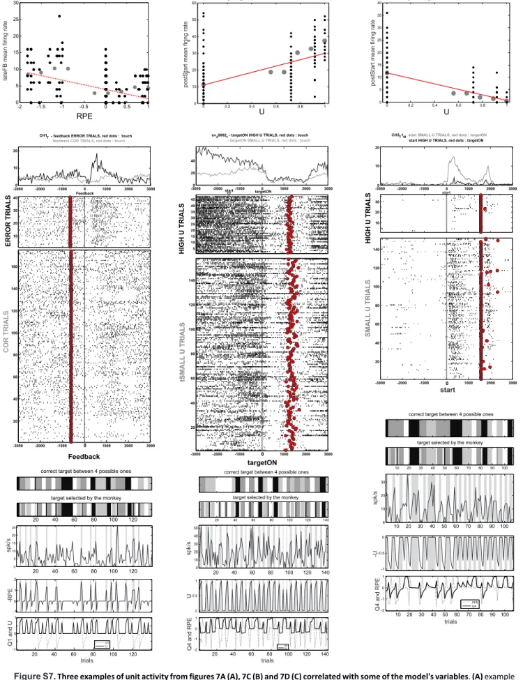
Model-based analysis of single-unit data. To test whether single units encoded information related to model computations, we used the following model variables as regressors of trial-by-trial activity: the reward prediction error [δ], the action value [Q] associated to each target and the outcome uncertainty [U]. The latter is a performance monitoring measure which assesses the

entropy of the probability over the different possible outcomes (i.e. reward

r

r

at the current trial t given the set

T

 

t

P

 

r

T



P

 

r

T

  

P

r

T



P

 

r

T



U





log



log

possible targets, U starts at a low value since there is 75% chance of making an error. U increases trial after trial during the search period. It is maximal when there remain 2 possible targets because there is 50% chance of making an error. Then U drops after either the first rewarded trial or the third error trial – because the fourth target is necessarily the rewarded one – and remains at zero during the repetition period. We decided to use a regressor with this pattern of change because it is somewhat comparable to the description of changes in frontal activity previously observed during the PS task (Procyk et al., 2000; Procyk and Goldman-Rakic, 2006).

We used U as the simplest possible parameter-free performance monitoring regressor for neural activity. This was done in order to test whether dACC and LPFC single-unit could reflect performance monitoring processes in addition to responding to feedback and tracking target values. But we note that the profile of U in this task would not be different from other performance monitoring measures such as the outcome history that we previously used in our computational model for dynamic control regulation in this task (Khamassi et al. 2011), or such as the vigilance level in the model of Dehaene and Changeux (Dehaene et al. 1998) which uses error and correct signals to update a regulatory variable (increased after errors and decreased after correct trials). We come back to possible interpretations of neural correlates of U in the discussion.

To investigate how neural activity was influenced by action values [Q], reward prediction errors [δ] as well as the outcome uncertainty [U], we performed a multiple regression analysis combined with a bootstrapping procedure, focusing our analyses on spike rates during a set of trial epochs (Fig. 1C): pre-start (0.5 s before trial start); post-start (0.5 s after trial start); pre-target (0.5 s before target onset); post-target (0.5 s after target onset); the action epoch defined as pre-touch (0.5 s before screen touch); pre-feedback (0.5 s before feedback onset); early-feedback (0.5 s after feedback onset); late-feedback (1.0 s after feedback period); inter-trial-interval (ITI; 1.5 s after feedback onset).

The spike rate y(t) during each of these intervals in trial t was analyzed using the following multiple linear regression model:

14

)

(

)

(

)

(

)

(

)

(

)

(

)

(

t

Q

t

Q

t

Q

t

Q

t

t

U

t

y































where

Q

(

t

),



k





1

...

4





is the reward prediction error, U(t) is the outcome uncertainty, and



,



i



 

1

...

n



coefficients.

δ, Q and U were all updated once in each trial. δ was updated at the time of feedback, so that regression analyses during pre-feedback epochs were done using δ from the previous trial, while analyses during post-feedback epochs used the updated δ. Q and U were updated at the end of the trial so that regression analyses in all trial epochs were done using the Q-values and U value of the current trial.

Note that the action value functions of successive trials are correlated, because they are updated iteratively, and this violates the independence assumption in the regression model. Therefore, the statistical significance for the regression coefficients in this model was determined by a permutation test. For this, we performed a shuffled permutation of the trials and recalculated the regression coefficients for the same regression model, using the same meta-parameters of the model obtained for the unshuffled trials. This shuffling procedure was repeated 1000 times (bootstrapping method), and the p value for a given independent variable was determined by the fraction of the shuffles in which the magnitude of the regression coefficient from the shuffled trials exceeded that of the original regression coefficient (Seo and Lee 2009), corrected for multiple comparisons with different model variables in different trial epochs (Bonferroni correction).

To assess the quality of encoding of action value information by dACC and LPFC neurons, we also performed a multiple regression analysis on the activity of each neuron related to Q-values after excluding trials where the preferred target of the neuron was chosen by the monkey. This analysis was performed to test whether the activity of such neurons still encodes Q-values outside trials where the target is selected. Similarly, to evaluate the quality of reward prediction error encoding, we performed separate multiple regression analyses on correct trials only versus error trials only. This analysis was performed to test whether the activity of such neurons quantitatively discriminate between different amplitudes of positive reward prediction errors and between different amplitudes of negative reward prediction errors. In both cases, the significance level of the multiple regression analyses was determined with a bootstrap method and a Bonferroni correction for multiple comparisons.

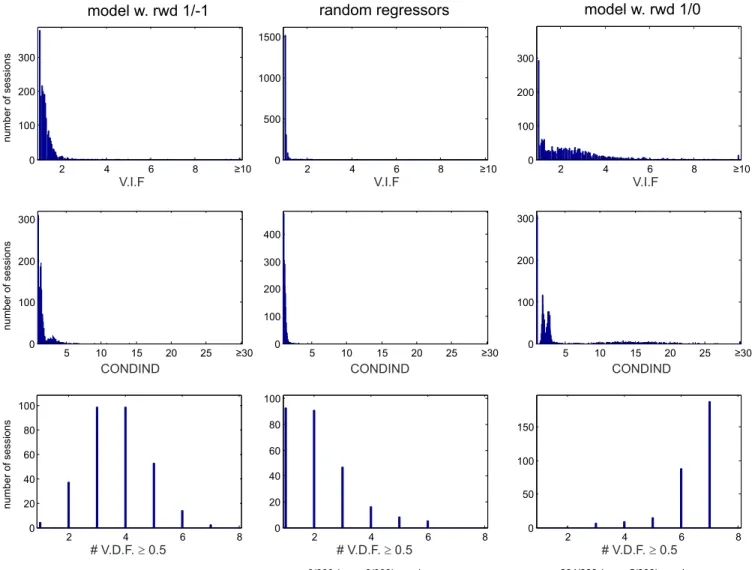
Finally, to measure possible collinearity issues between model variables used as regressors of neural activity, we used Brian Lau’s Collinearity Diagnostics Toolbox for Matlab

(http://www.subcortex.net/research/code/collinearity-diagnostics-matlab-code (Lau 2014)). We

15

when each regressor was expressed as a function of the other regressors. We also computed the condition indexes (CONDIND) and variance decomposition factors (VDF) obtained in the same analysis. A strong collinearity between regressors was diagnosed when CONDIND ≥ 30 and more than two VDFs > 0.5. A moderate collinearity was diagnosed when CONDIND ≥ 10 and more than two VDFs > 0.5. CONDIND ≤ 10 indicated a weak collinearity.

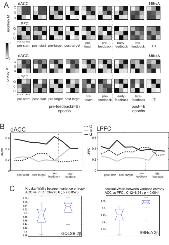
Principal component analysis. To determine the degree to which single-unit activity segregated or integrated information about model variables, we performed a Principal Component Analysis

(PCA) on the 3 correlation coefficients



, 



i



4

...

6





and relating neural activity with the 3 main model variables (reward prediction error δ, outcome

uncertainty U, and the action value Qk associated to the animal’s preferred target k). For each trial

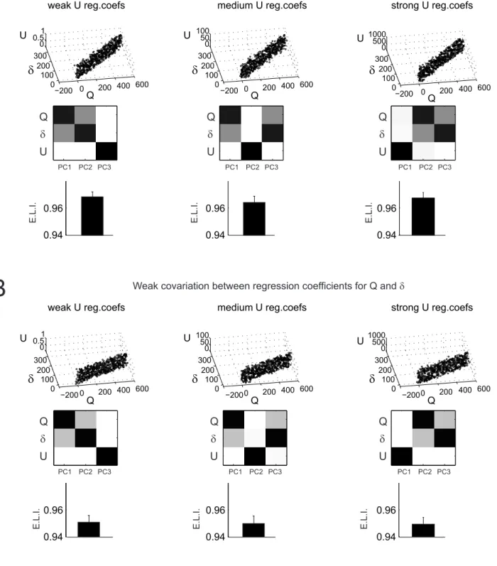
epoch, we pooled the coefficients obtained for all neurons in correlation with these model variables. Each principal component being expressed as a linear combination of the vector of correlation coefficients of neuron activities with these three model variables, the contribution of different model variables to each component gives an idea as to which extent cell activity is explained by an integrated contribution of multiple model variables. For instance, if a PCA on cell activity in the early-delay period produces three principal components that are each dependent on a different single model variable (e.g. PC1 = 0.95Q + 0.01δ + 0.04U; PC2 = 0.1Q + 0.8δ + 0.1U; PC3 = 0.05Q + 0.05δ + 0.9U), then activity variations are best explained by separate influences from the information conveyed by the model variables. If in contrast, the PCA produces principal components which strongly depend on multiple variables (e.g. PC1 = 0.5Q + 0.49δ + 0.01U; PC2 = 0.4Q + 0.1δ + 0.5U; PC3 = 0.2Q + 0.4δ + 0.4U), then variations of the activities are best explained by an integrated influence of such information (see Supplementary Figure S1 for illustration of different Principal Components resulting from artificially generated data showing different levels of integration between model variables).

We compared the normalized absolute values of the coefficients of the three principal components so that a coefficient close to 1 denotes a strong correlation while a coefficient close to 0 denotes no correlation. To quantify the integration of information about different model variables in single-unit activities, for each neuron k, we computed an entropy-like index (ELI) of sharpness of encoding of different model variables based on the distributions of regression coefficients between cell activities and model variables:

 



Where ci is the absolute value of the z-scored correlation strength ρi with model variable i. A neuron with activity correlated with different model variables with similar strengths will have a high

16

ELI; a neuron with activity highly correlated with only one model variable will have a low ELI. We compared the distributions of ELIs between dACC and LPFC in each trial epoch using a Kruskal-Wallis test.

Finally, we estimated the contribution of each model variable to neural activity variance in each epoch and compared it between dACC and LPFC. To do so, we first normalized the coefficients for each principal component in each epoch. These coefficients being associated to three model variables Q, δ and U, this provided us with a contribution of each model variable to each principal component in each epoch. We then multiplied them by the contribution of each principal component to the global variance in neural activity in each epoch. The result constituted a normalized contribution of each model variable to neural activity variance in each epoch. We finally computed the entropy-like index (ELI) of these contributions. We compared the set of epoch-specific ELI between dACC and LPFC with a Kruskal-Wallis test.

Mutual information. We measured the mutual information between monkey's choice at each trial and the firing rate of each individual recorded neuron during the early-delay epoch ([ST+0.1s;

ST+1.1s]). The mutual information (IS;R) was estimated by first computing a confusion matrix (Quian

Quiroga and Panzeri 2009), relating at each trial t, the spike count from the unit activity in the early-delay epoch (as “predicting response” R) and the target chosen by the monkey (i.e. 4 targets as “predicted stimulus” S). Since neuronal activity was recorded during a finite number of trials, not all possible response outcomes of each neuron to each stimulus (target) have been sufficiently sampled. This is called the “limited sampling bias” which can be overcome by subtracting a correction term from the plug-in estimator of the mutual information (Panzeri et al. 2007). Thus we subtracted the Panzeri Treves (PT) correction term (Treves and Panzeri 1995) from the estimated mutual information

) R ; S (I :











 



_

Where N is the number of trials during which the unit activity was recorded, R is the number of

relevant bins among the M possible values taken by the vector of spike counts and computed by the

“bayescount” routine provided by (Panzeri and Treves 1996), and RS is the number of relevant

responses to stimulus (target) s.

Such measurement of information being reliable only if the activity was recorded during a sufficient number of trials per stimulus presentation, we restricted this analysis to units that verified the following condition (Panzeri et al. 2007):

4 R /

N_S  (16)

17

Finally, to verify that such a condition was sufficiently restrictive to exclude artifactual effects, for each considered neuron we constructed 1000 pseudo response arrays by shuffling the order of trials at fixed target stimulus, and we recomputed each time the mutual information in the same manner (Panzeri et al. 2007). Then we verified that the average mutual information obtained with such shuffling procedure was close to the PT bias correction term computed with Equation 15 (Panzeri and Treves 1996).

RESULTS

Previous studies have emphasized the role of LPFC in cognitive control and dACC in adjustment of action values based on measures of performance such as reward prediction errors, error-likelihood and outcome history. In addition, variations of activities in the two regions between exploration and exploitation suggest that both contribute to the regulation of the control level during exploration. Altogether neurophysiological data suggest particular relationships between dACC and LPFC, but their respective contribution during adaptation remains unclear and a computational approach to this issue appears highly relevant. We recently modeled such relationships using the meta-learning framework (Khamassi et al. 2011). The network model was simulated in the Problem Solving (PS) task (Quilodran et al., 2008) where monkeys have to search for the rewarded target in a set of four on a touch-screen, and have to repeat this rewarded choice for at least 3 trials before starting a new search period (Fig. 1A). In these simulations, variations of the model’s control meta-parameter (i.e. inverse temperature β) produced variations of choice selectivity in simulated LPFC in the following manner: a decrease of choice selectivity (exploration) during search; an increase of choice selectivity (exploitation) during repetition. This resulted in a globally higher mean choice selectivity in simulated LPFC compared to simulated dACC, and in a co-variation between choice selectivity and the inverse temperature in simulated LPFC but not in simulated dACC (Khamassi et al. 2011). This illustrates a prediction of computational models on the role of prefrontal cortex in exploration (McClure et al. 2006; Cohen J. D. et al. 2007; Krichmar 2008) which has not yet been tested experimentally.

Characteristics of behaviors

To assess the plausibility of such computational principles we first analyzed animals’ behavior in the PS task. During recordings, monkeys performed nearly optimal searches, i.e., rarely repeated incorrect trials (INC), and on average made errors in less than 5% of repetition trials. Although the animals' strategy for determining the correct target during search periods was highly efficient, the pattern of successive choices was not systematic. Analyses of series of choices during search periods revealed that monkeys used either clockwise (e.g. choosing target 1 then 2), counterclockwise, or

18

crossing (going from one target to the opposite target in the display, e.g. from 1 to 3) strategies, with a slightly higher incidence for clockwise and counterclockwise strategies, and a slightly higher incidence for clockwise over counterclockwise strategy (Percent clockwise, counterclockwise, crossing and repeats were 38%, 36%, 25%, 1% and 39%, 33%, 26%, 2% for each monkey respectively, measured for 9716 and 4986 transitions between two targets during search periods of 6986 and 3227 problems respectively). Rather than being systematic or random, monkeys’ search behavior appeared to be governed by more complex factors: shifting from the previously rewarded target in response to the Signal to Change (SC) at the beginning of most new problems (Fig. 2A-middle); spatial biases i.e. more frequent selection of preferred targets in the first trial of search periods (Fig. 2A-right); and efficient adaption to each choice error as argued above. This indicates a planned and controlled exploratory behavior during search periods. This is also reflected in an incremental change in reaction times during the search period, with gradual decreases after each error (Fig. 2B). Moreover, reaction times shifted from search to repetition period after the first reward (CO1), suggesting a shift between two distinct behavioral modes or two levels of control (Monkey M: Wilcoxon Mann-Whitney U-test, p < 0.001; Monkey P: p < 0.001; Fig. 2B).

Model-based analyses. Behavioral analyses revealed that monkeys used nearly-optimal strategies to solve the task, including shift at problem changes, which are unlikely to be solved by simple reinforcement learning. In order to identify the different elements that took part in monkey's decisions and adaptation during the task we compared the fit scores of several distinct models to trial-by-trial choices after estimating each model’s free meta-parameters that maximize the log-likelihood separately for each monkey (see Methods). We found that models performing either a random search or a clockwise search and then simply repeating the correct target could not properly reproduce monkeys' behavior during the task, even when the clockwise search was systematically

started by the monkeys' preferred target according to its spatial biases (Models RandS _and ClockS;

Table 1 and Fig. 2D). Moreover, the fact that monkeys most often shifted their choice at the beginning of each new problem in response to the Signal to Change (SC) (Fig. 2A-middle) prevented a simple reinforcement learning model (Q-learning) or even a generalized reinforcement learning model from reproducing monkey's behavior (resp. QL and GQL in Table 1). Indeed, these models obviously have a strong tendency to choose the previously rewarded target without taking into account the Signal to Change to a new problem. Behavior was better reproduced with a combination of generalized reinforcement learning and reset of target values at each new problem (shifting the previously rewarded target and taking into account the animal's spatial biases measured during the previous session; i.e. Models GQLSB, GQLSB2β, SBnoA, SBnoA2β in Figure 2D and Table 1). We tested

19

control models without spatial biases, without problem shift, and with neither of them, to show that they were both required to fit behavior (resp. GQLSnoB, GQLBnoS and GQLnoSnoB in Table 1). We also tested a model with spatial biases and shift but without progressive updating of target values

nor forgetting – i.e.





1

,





1

SBnoA with 1 less meta-parameter) and found that it was not as good as SBnoA in fitting monkeys’ behavior, as found with a likelihood ratio test at p=0.05 with one degree of freedom.

Although Models GQLSB, GQLSB2β, SBnoA, SBnoA2β were significantly better than other tested models along all used criteria (maximum likelihood [Opt-LL], BIC score, AIC score, log of posterior probability [LPP], out-of-sample test [Test-LL] in Table 1), these 4 versions gave similar fit performance. In addition, the best model was not the same depending on the considered criterion: Model GQLSB2β was the best according to LL, BIC and AIC scores, and second best according to LPP and Test-LL scores; Model SBnoA2β was the best according to LPP score; Model GQLSB was the best according to Test-LL score.

As a consequence, the present dataset does not allow to decide whether allowing a free meta-parameter α (i.e. learning rate) in model GQLSB and GQLSB2β is necessary or not in this task, compared to versions of these models where α is fixed to 1 (Model SBnoA and SBnoA2β) (Fig. 2D and Table 1). This is due to the structure of the task – where a single correct trial is sufficient to know which is the correct target – which may be solved by sharp updates of working memory rather than by progressive reinforcement learning (although a small subset of the sessions were better fitted

with 





Supplementary Fig. S2). We come back to this issue in the discussion.

Similarly, models that use distinct control levels during search and repetition (Models GQLSB2β and SBnoA2β) could not be distinguished from models using a single parameter (Models GQLSB and SBnoA) in particular because of out-of-sample test scores (Table 1).

Nevertheless, model-based analyses of behavior in the PS task suggest complex adaptations possibly combining rapid updating mechanisms (i.e. α close to 1), forgetting mechanisms and the use of information about the task structure (Signal to Change; first correct feedback signaling the beginning of repetition periods). Model GQLSB2β here combines these different mechanisms in the more complete manner and moreover won the competition against the other models according to three criteria out of five. Consequently, in the following we will use Model GQLSB2β for model-based analyses of neurophysiological data and will systematically compare the results with analyses performed with Models GQLSB, SBnoA, SBnoA2β to verify that they yield similar results.

In summary, the best fit was obtained with Models SBnoA, SBnoA2β, GQLSB, GQLSB2β which could predict over 80% of the choices made by the animal (Table 1). Figure 2A shows a sample of

20

trials where Model SBnoA can reproduce most monkey choices, and illustrating the sharper update of action values in Model SBnoA (with α = 1) compared to Model GQLSB (where the optimized α = 0.7). When freely simulated on 1000 problems of the PS task – i.e., the models learned from their own decisions rather than trying to fit monkeys’ decisions –, the models made 38.23% clockwise search trials, 32.41% counter-clockwise, 29.22% crossing and 0.15% repeat. Simulations of the same models without spatial biases produced less difference between percentages of clockwise, counter-clockwise and crossing trials, unlike monkeys: 33.98% counter-clockwise, 32.42% counter-counter-clockwise, 33.53% crossing and 0.07% repeat.

Distinct control levels between search and repetition. To test whether behavioral adaptation could be described by a dynamical regulation of the β meta-parameter (i.e. inverse temperature) between search and repetition, we analyzed the value of the optimized two distinct free

meta-parameters (βS and βR) in Models GQLSB2β and SBnoA2β (Fig. 2E, 2C and Suppl. Fig. S2). The value of

the optimized βS and βR meta-parameters obtained for a given monkey in a given session constituted

a quantitative measure of the control level during that session. Such level was non-linearly linked to

the number of errors the animal made. For instance, a βR of 3, 5, or 10 corresponded to

approximately 20%, 5%, and 0% errors respectively made by the animal during repetition periods (Fig. 2C).

Interestingly, the distributions of βS and βR obtained for each recording session showed

dissociations between search and repetition periods in a large number of sessions. We found a

unimodal distribution for the β meta-parameter during the search period (βS), reflecting a consistent

level of control in the animal behavior from session to session. In contrast, we observed a bimodal

distribution for the β meta-parameter during the repetition period (βR; Fig. 2E). In Figure 2E, the

peak on the right of the distribution (large βR) corresponds to a subgroup of sessions where behavior

shifted between different control levels from search to repetition periods. This shift in the level of control could be interpreted as a shift from exploratory to exploitative behavior, an attentional shift or a change in the working memory load, as we discuss further in the Discussion. Nevertheless this is consistent with the hypothesis of a dynamical regulation of the inverse temperature β between search and repetition periods in this task (Khamassi et al. 2011; Khamassi et al. 2013). The bimodal

distribution for βR illustrates the fact that during another subgroup of sessions (small βR), the animal’s

behavior did not shift to a different control level during repetition and thus made more errors. Such bimodal distribution of the β meta-parameter enables to separate sessions in two groups and to compare dACC and LPFC activities (see below) during sessions where decisions displayed a shift and

21

crucially dependent of the optimized learning rate α since a similar bimodal distribution was

obtained with Model SBnoA2β and since the optimized βS and βR values in the two models were

highly correlated (N = 277; βS: r = 0.9, p < 0.001; βR: r = 0.96, p < 0.001; Supplementary Fig. S2).

Modulation of information coding

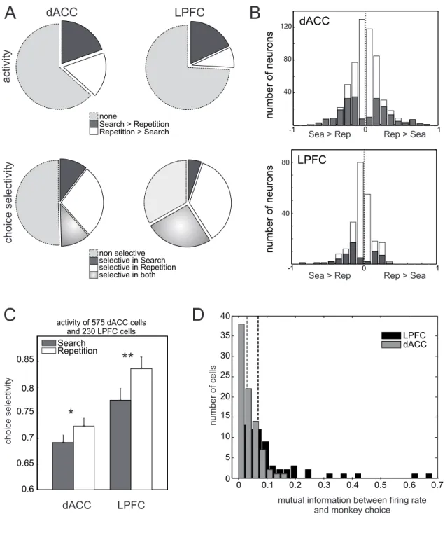
To evaluate whether a behavioral change between search and repetition was accompanied by changes in LPFC activity and choice selectivity, we analyzed a pool of 232 LPFC single-units (see Fig. 1B for the anatomy) in animals performing the PS task, and compared the results with 579 dACC single-unit recordings which have been only partially used for investigating feedback-related activity (Quilodran et al. 2008). We report here a new study relying on comparative analyses of dACC and LPFC responses, the analysis of activities before the feedback – especially during the delay period –, and the model-based analysis of these neurophysiological data. The results are summarized in Supplementary Table 1.

Average activity variations between search and repetition. Previous studies revealed differential prefrontal fMRI activations between exploitation (where subjects chose the option with maximal value) and exploration trials (where subjects chose a non-optimal option) (Daw N. D. et al. 2006). Here a global decrease in average activity level was also observed in the monkey LPFC from search to repetition. For early-delay activity, the average index of variation between search and repetition in LPFC was negative (mean: -0.05) and significantly different from zero (mean: t-test p < 0.001, median: Wilcoxon Mann-Whitney U- test p < 0.001). The average index of activity variation in dACC was not different from zero (mean: -0.008; t-test p > 0.35; median: Wilcoxon Mann-Whitney U- test p > 0.25). However, close observation revealed that the non-significant average activity variation in dACC was due to the existence of equivalent proportions of dACC cells showing activity increase or activity decrease from search to repetition, leading to a null average index of variation (Fig. 3A-B; 17% versus 20% cells respectively). In contrast, more LPFC single units showed a decreased activity from search to repetition (18%) than an increase (8%), thus explaining the apparent global decrease of average LPFC activity during repetition. The difference in proportion between dACC and LPFC is

significant (Pearson χ2 test, 2 df, t = 13.0, p < 0.01) and was also found when separating data for the

two monkeys (Supplementary Fig. S3). These changes in neural populations thus suggest that global non-linear dynamical changes occur in dACC and LPFC between search and repetition instead of a simple reduction or complete cessation of involvement during repetition.

Modulations of choice selectivity between search and repetition. As shown in Figure 3A, a higher proportion of neurons showed a significant choice selectivity in LPFC (155/230, 67%) than in dACC

22

(286/575, 50%; Pearson χ2 _{test, 1 df, t = 20.7, p < 0.001) – as measured by the vector norm in}

Equation 10. Interestingly, the population average choice selectivity was higher in LPFC (0.80) than in dACC (0.70; Kruskal-Wallis test, p < 0.001; see Fig. 3C). When pooling all sessions together, this resulted in a significant increase in average choice selectivity in LPFC from search to repetition (mean variation: 0.04; Wilcoxon Mann-Whitney U-test p < 0.01; t-test p < 0.01; Fig. 3C).

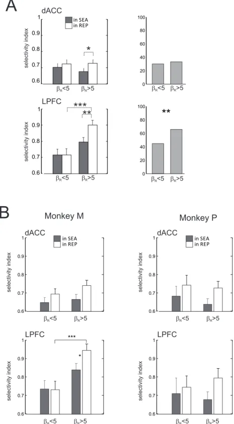
Strikingly, the significant increase in LPFC early-delay choice selectivity from search to repetition was found only during sessions where the model fit dissociated control levels in search and repetition (i.e. sessions with large βR [βR > 5]; Kruskal-Wallis test, 1df, χ2 = 6.45, p = 0.01; posthoc test with Bonferroni correction indicated that repetition > search). Such an effect was not found during sessions where the model reproducing the behavior remained at the same control level during repetition (i.e. sessions with small βR [βR < 5]; Kruskal-Wallis test, p > 0.98) (Fig. 4-bottom).

Interestingly, choice selectivity in LPFC was significantly higher during repetition for sessions

where βR was large (mean choice selectivity = 0.91) than for sessions where βR was small (mean

choice selectivity = 0.73; Kruskal-Wallis test, 1df, χ2 = 12.5, p < 0.001; posthoc test with Bonferroni

correction; Fig. 4-bottom). Thus, LPFC early-delay choice selectivity clearly covaried with the level of control measured in the animal’s behavior by means of the model.

There was also an increase in dACC early-delay choice selectivity between search and repetition consistent with variations of β, but only during sessions where the model capturing the animal’s

behavior made a strong shift in the control level (βR > 5; mean variation = 0.035, Kruskal-Wallis test,

1df, χ2 = 5.22, p < 0.05; posthoc test with Bonferroni correction indicated that repetition > search; Fig.

4-top). However, overall, dACC choice selectivity did not follow variations of the control level.

Two-way ANOVAs either for (βS x task phase) or for (βR x task phase) revealed no main effect of β (p > 0.2),

an effect of task period (p < 0.01), but no interaction (p > 0.5). And there was no significant difference

in ACC choice selectivity during repetition between sessions with a large βR (mean choice selectivity =

0.69) and sessions with a low one (mean choice selectivity = 0.75; Kruskal-Wallis test, 1 df, χ2 = 3.11, p

> 0.05).

At the population level, increases in early-delay mean choice selectivity from search to repetition were due both to an increase of single unit selectivity, and to the emergence in repetition of selective units that were not significantly so in search (Fig. 3A). Importantly, the proportion of LPFC early-delay

choice selective neurons during repetition periods of sessions where βR was small (55%) was

significantly smaller than the proportion of such LPFC neurons during sessions where βR was large

(72%; Pearson χ2 test, 1 df, t = 7.19, p < 0.01). In contrast, there was no difference in proportion of

dACC early-delay choice selective neurons during repetition between sessions where βR was small