Extrasolar Planets with AMBER/VLTI, What can we expect from current performances ?

(1)

HAL Id: hal-00015058

https://hal.archives-ouvertes.fr/hal-00015058

Submitted on 9 Dec 2005

HAL is a multi-disciplinary open access

archive for the deposit and dissemination of

sci-entific research documents, whether they are

pub-lished or not. The documents may come from

teaching and research institutions in France or

abroad, or from public or private research centers.

L’archive ouverte pluridisciplinaire HAL, est

destinée au dépôt et à la diffusion de documents

scientifiques de niveau recherche, publiés ou non,

émanant des établissements d’enseignement et de

recherche français ou étrangers, des laboratoires

publics ou privés.

Extrasolar Planets with AMBER/VLTI, What can we

expect from current performances ?

Florentin Millour, Martin Vannier, R. Petrov, Bruno Lopez, Frederik

Rantakiro

To cite this version:

Florentin Millour, Martin Vannier, R. Petrov, Bruno Lopez, Frederik Rantakiro. Extrasolar Planets

with AMBER/VLTI, What can we expect from current performances ?. Direct Imaging of Exoplanets:

Science & Techniques., 2006, Nice, France. pp.291-296, �10.1017/S1743921306009471�. �hal-00015058�

(2)

ccsd-00015058, version 1 - 9 Dec 2005

Proceedings IAU Colloquium No. xxx, 2005 A.C. Editor, B.D. Editor and C.E. Editor, eds.

c

2005 International Astronomical Union DOI: 00.0000/X000000000000000X

Extrasolar Planets with AMBER/VLTI,

What can we expect from current

performances ?

F. Millour

1;2

, M. Vannier

4

, R. G. Petrov

1

, B. Lopez

3

and

F. Rantakyr¨

o

4

1

Laboratoire Universitaire d’Astrophysique de Nice - U.M.R. 6525 Universit´e de Nice-Sophia Antipolis, Parc Valrose, 06108 Nice Cedex 02, France

2

Laboratoire d’Astrophysique de Grenoble, U.M.R. 5571

Universit´e Joseph Fourier/C.N.R.S., BP 53, F-38041 Grenoble Cedex 9, France

3

Laboratoire Gemini, U.M.R. 6203

Observatoire de la Cˆote d’Azur/C.N.R.S., Avenue Copernic, 06130 Grasse, France

4

European Southern Observatory Casilla 19001, Santiago 19, Chile

Abstract. We present the current performances of the AMBER / VLTI instrument in terms of differential observables (differential phase and differential visibility) and show that we are already able to reach a sufficient precision for very low mass companions spectroscopy and mass characterization. We perform some extrapolations with the knowledge of the current limitations of the instrument facility.

We show that with the current setup of the AMBER instrument, we can already reach 3σ = 10−3 _{radians and have the potential to some low mass companions characterization (Brown}

dwarves or hypothetical very hot Extra Solar Giant Planets). With some upgrades of the VLTI infrastructure, improvements of the instrument calibration and improvements of the observing strategy, we will be able to reach 3σ = 10−4 _{radians and will have the potential to perform}

Extra Solar Giant Planets spectroscopy and mass characterization.

Keywords.techniques: interferometric, stars: planetary systems, instrumentation: high angular resolution

1. Introduction

In this paper we discuss the current highest performances of Colour-Differential Inter-ferometry (CDI) on the AMBER instrument and compare these performances to signal amplitude we computed from low-mass companion simulations.

CDI is based on simultaneous interferometric observations in different spectral chan-nels. As a high-angular resolution and high-dynamic technique, it presents two major advantages. First, the chromatic differences in visibility and phases are much less sensi-tive to instrumental and atmospheric instabilities, and therefore are easier to calibrate than the absolute complex visibility. Since the beginning of long-baseline optical inter-ferometry with separated apertures, many early astrophysical results have been obtained using this self-calibration feature (Thom et al. 1986; Mourard et al. 1989). Second, the colour-differential phase can be measured with an accuracy much better than the angular interferometric resolution λ/B. For objects much smaller than the diffraction limit, it is proportional to the variation of the object photocentre with wavelength.

This paper is placed in the context of Extra Solar Planets characterization with inter-119

(3)

120 Millour, Petrov et al.

ferometry (Vannier et al. 2005) and is intending to show that this technique has already the potential to get some scientific results on high contrast binaries.

2. Differential Observables computation and error bars

2.1. The differential phase estimator

The expression of the coherent flux on tha AMBER instrument is (Millour et al. 2004):

C(t, λ) = 2N (λ)Vi(t, λ)V (λ)pp1(t, λ)p2(t, λ) v u u t Nx X k=1 a1k(λ)a2k(λ)×eφi(t,λ)+φp(t,λ)+φo(t,λ)+φc(t,λ) (2.1) In this equation k is the pixel index (spatial direction), N (λ) is the unknown object’s flux, p1(t, λ) and p2(t, λ) are transmission coefficients for the two combined beams, and a1k(λ) and a2k(λ) are related to specific features of each pixel (shape of the beam). Vi(t, λ) is the instrumental contrast and V (λ) is the amplitude of the complex visibility. φp(t, λ) is the phase induced by the achromatic piston, φi(t, λ) is the instrumental-induced phase that varies with time (since the fixed part is already removed by the data reduction algorithm of AMBER as explained in Millour et al. (2004)), φo(t, λ) is the observed object’s phase and φc(t, λ) is the chromatic phase induced by other causes (Chromatic atmospheric phase for example).

If we suppose that φi(t, λ) = 0 (no variable instrumental phase), φc(t, λ) = 0 (no chromatic effect) and φo(t, λ) = 0 (unresolved or centro-symmetric object) then we can correct the complex coherent flux from the achromatic piston effect by:

Cnop(t, λ) = C(t, λ) × e−2iπδ(t)

λ (2.2)

One can note that we need an estimation of the achromatic piston for each sample of time. This is a part of the Ph.D. thesis of Eric Tatulli (Tatulli 2004) and it will not be explained in detail in this article. We compute a reference channel for each spectral channel, taking care of non biasing the interspectral term by removing the “work” spectral channel before averaging:

Cref(t, λk) = hCnop(t, λi)iλ_i6=λk (2.3)

We compute then the interspectral term between this reference spectral channel and the work spectral channel:

W (λk) = Cnop(t, λk)Cref(t, λk)∗ |Cref(t, λk)|2 (t) (2.4) Then we compute the differential phase:

φdiff(λ) = arg(W (λ)) (2.5) This expression of the differential phase is quite accurate with a good achromatic piston correction. That is why it can be applied only to high flux sources (for example the star 51 Peg. has a K magnitude of 5, which is sufficient for this type of application). We can express the interspectral term by:

(4)

Please note that when φo(t, λ) cannot be neglected with regards to φp(t, λ), then the expression of the differential phase is different and contains a bias related to the interferometric phase, which leads to a bias in W (λ). For well resolved objects, this effect has to be taken into account and leads to a specific treatment. Thus it is well beyond the scope of this paper and will be discussed in a futher one.

2.2. The differential visibility estimator

Going back to the interspectral term evaluation 2.4, we see that its modulus can be expressed as: V_V(λ)_ref . If we have an unbiased estimate of this modulus (which we call

g

Vdiff(λ)), then we can compute the differential visibility. This estimate can be made with the real part of the differential phase correction of the interspectral term:

g

Vdiff(λ) = ℜ(W (λ) × e−iφdiff(λ)₎ _(2.7)

This estimate of the differential visibility is unbiased as we expect the visibility and phase to be uncorrelated.

2.3. The error bars 2.3.1. In theory

Starting from the theoretical estimation of the differential phase, we can express the differential phase and visibility noises from the fundamental photon√N∗, thermal√Nth and detector σRON√nfnpix noises (Petrov 1989).

σΦ= p (N∗+ Nth+ nfnpixσ2 RON)/2 V hNi (2.8) σV = p N∗+ Nth+ nfnpixσ2 RON hNi (2.9)

For information, the closure phase noise is given by:

σψ=√3 × σΦ (2.10) 2.3.2. in practice

For the practical error computation, we perform a statistical dispersion of the observed points and assume a gaussian noise. The expression of the estimated noise for each observable is then the standard deviation of the measurements over an exposure:

σX = s Pnf 1 (X − hXi)2 n2 f (2.11)

3. Typical expected signal

3.1. Simulating the companion

We simulated a standard binary star model as in eq. 3.1 and applied the computation we currently use on the AMBER instrument to extract differential visibilities, differential phases and closure phase, computed the error bars assuming an average instrumental contrast of 50%, 1000 frames of integration, a detector noise of 11e− _{per pixel and per} frame and a total photon count of 4.2 × 107_{, the same figures as in the following section.}

(5)

Cjk(λ) = 1 + R(λ)e

−2iπ−→_{ujk ·}−→_ρ

1 + R(λ) (3.1) We used a modeled exoplanet spectrum from Barman et al. (2001) convolved with the resolution of the AMBER instrument in LR mode (R ≈ 35). We scaled this flux ratio to a maximum value of ≈ 10−3 _{in order to estimate the signal amplitude of a 10 times} brighter companion.

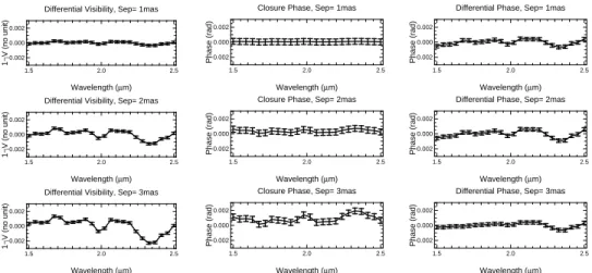
1.5 2.0 2.5

−0.002 0.000 0.002

Differential Visibility, Sep= 1mas

Wavelength (µm) 1−V (no unit) 1.5 2.0 2.5 −0.002 0.000 0.002

Closure Phase, Sep= 1mas

Wavelength (µm) Phase (rad) 1.5 2.0 2.5 −0.002 0.000 0.002

Differential Phase, Sep= 1mas

Wavelength (µm)

Phase (rad)

Figure 1. Simulations of an observation at VLTI with UT1-UT3-UT4 showing from left to right the differential visibility, the closure phase and the differential phase and from top to bottom separations ranging 1 to 3 mas. It shows a clear signal for all observables at 3mas but none for the closure phase at 1mas whereas the visibility and phase still have detectable signal. Photon amount is 4.2 × 107

, detector noise 11e−_{, number of frames 1000, number of pixels 32}

and average visibility 50%. These plots evidence the “super resolution” properties of differental phase and visibility relatively to closure phase.

3.2. Results

We tested the obtained signal for several Star/Companion separations and found that the signal detection at 3σ would occur for a separation of only 1mas for differential phase and visibility and 2.5mas for closure phase. This effects is due to the fact that if we perform a 1st _{order taylor expansion of the phase, we get a linear dependence with} −→

ujk· −→ρ whereas for visibility, we get a squared dependence and for the closure phase we get a cubic dependence. So for small separations, we have φdiff > Vdiff > ψ.

4. Best performances of AMBER

We used the AMBER / VLTI instrument to observe the bright calibration star HD70060 at low spectral resolution during the GTO run of 25 december 2004. We used the tech-nique explained below to compute the differential phases and differential visibilities and computed statistical error bars. These ones were compared to the theoretical ones as-suming a detector noise of 11 electrons and a null thermal noise. The figure 2 shows the resulting average differential phases for 5 successive exposures where we selected 50% of the best frames using the finge SNR as selection criterion. Each exposure represents about 20s of observation. They are separated by about 60 s.

(6)

phase per spectral channel as described in eq. 2.11. We performed weighted averages using the SNR on the fringe signal as weights. nφ is the total number of collected photons per spectral channel and σφ is the accuracy expected from measured flux, detector noise and a supposed object visibility of 1 (which means the measured visibility is supposed to be only the instrumental one).

A A A A A B B B B B C C C C C D D D D E E E E 2.05 2.10 2.15 2.20 10−6 −0.1 0.0 0.1 file A σ=3.58e−03 nφ=2.30e+06 σφ=8.96e−04 file B σ=3.07e−03 nφ=2.15e+06 σφ=9.42e−04 file C σ=6.95e−03 nφ=2.07e+06 σφ=9.69e−04 file D σ=2.87e−03 nφ=2.59e+06 σφ=8.22e−04 file E σ=3.71e−03 nφ=2.84e+06 σφ=7.69e−04 Wavelength (m) 1 − V A A A A A A B B B B B B C C C C C C C D D D D D D E E E E E E 2.05 2.10 2.15 2.20 10−6 0.00 0.05 file A σ=1.69e−03 nφ=2.30e+06 σφ=8.61e−04 file B σ=1.70e−03 nφ=2.15e+06 σφ=9.18e−04 file C σ=3.14e−03 nφ=2.07e+06 σφ=1.05e−03 file D σ=1.54e−03 nφ=2.59e+06 σφ=7.51e−04 file E σ=1.53e−03 nφ=2.84e+06 σφ=7.15e−04 TOTAL σ=7.47e−04 nφ=1.19e+07 σφ=3.72e−04 K mag = 4.063 Wavelength (m) Phase (rad)

Figure 2. Differential Visibilities and Phases of the calibrator star HD70060 for 5 successive exposures (lines with letters) and the resulting average of the 5 exposures (thick line).

4.1. Differential Visibility

The differential visibility values vary only by 4 × 10−3 _{with time within each exposure} but the general slope of the curve changes dramatically between exposure, leading to a variation of about 0.05 radians rms over 5 minutes. This variation is dominated by the changes in the achromatic piston jitter due to seeing and vibrations fluctuations. In the current VLTI situation we have no tool to correct this effect, except including an estimation of the exposure jitter in the model fitting, with an impact on the SNR which cannot be estimated. So the differential visibility is currently not usable for very high accuracy applications. This situation will change dramatically when a fringe tracker is operational. Then we will be affected only by the residual piston jitter after fringe tracking correction.

4.2. Differential Phase

The rms variation of the measures within each exposure is of typically 1.8 milliradians (i.e. ≈ 1µarcsecond in colour-differential astrometry). This is about two times the expected rms from fundamental noise. Over the total 5 minutes we get 0.9 milliradians, again very close to twice the photon noise. This shows that the different measures seems statistically independent. An average of 1200 such exposures (15 hours) is needed to reach the 0.5 × 10−4accuracy needed for the spectroscopy of τ Bootis b. The brighter planet considered in §3 could be observed in 1 hour.

With the improvement of the VLTI (less vibrations, improved overheads) we could expect to use almost all frames instead of only 50% of them with an average instrumental contrast improved by a factor 2. Then the τ Boo observation would be achievable in a couple of hours. We also see a pattern as a function of lambda with a 10−2 radians rms over the K band. This pattern is stable over the 5 minutes of observations considered

(7)

here. That means that it can be eliminated by a fast calibration cycle. We think that it is a mixture of atmospheric dispersion and measurement effects. Measurement effects can be eliminated by beam commutation. Atmospheric dispersion will be eliminated in the closure phase and we plan to try to fit it in the differential phase.

4.3. Closure Phase

In this relatively poor quality early data, we have too little frames where the three fringe patterns are good enough. This explains why the closure phase is much more noisy (typically 10−2_{radians rms) than the differential phases. We are therefore unable to say} what part of the differential phase pattern is due to differential chromatic OPD.

5. Conclusion

The preliminary data reduction of bright sources observed in low spectral resolution with AMBER shows that the measured differential phases are accurate and stable enough to achieve the spectroscopy and angular separation of the most favorable Pegasi planets in a few 15 hours observations. This value should be reduced to 2 hours with the fore-seen simple improvements of the VLTI. The resulting spectra would be affected by an instrumental term and/or an atmospheric chromatic differential OPD term producing a smooth 10−2 radians pattern over the K band.

When the instrumental term will be eliminated by beam commutation, the remaining differential OPD might be possible to fit in the data reduction procedure. However, only a successful use of closure phase guarantees the elimination of the differential OPD. The current quality of the VLTI does not allow accurate closure phase measurements, but this should be improved soon, when the three fringe pattern are better stabilized. We remain very optimistic about the possibility to do spectroscopy of Pegasi planets with AMBER quite sson.

Acknowledgements

The data presented here was taken at the Paranal Observatory in Chile within the AMBER Guaranteed Time.

We thank all the consortium members listed in http://amber.obs.ujf-grenoble.fr.

References

Barman, T. S., Hauschildt, P. H., & Allard, F. 2001, ApJ, 556, 885

Millour, F., Tatulli, E., Chelli, A. E., et al. 2004, in New Frontiers in Stellar Interferometry., ed. W. A. Traub., Vol. 5491 (SPIE), 1222–+

Mourard, D., Bosc, I., Labeyrie, A., Koechlin, L., & Saha, S. 1989, Nature, 342, 520

Petrov, R. G. 1989, in NATO ASIC Proc. 274: Diffraction-Limited Imaging with Very Large Telescopes, 249–+

Tatulli, E. 2004, PhD thesis, Universit´e Joseph Fourier Thom, C., Granes, P., & Vakili, F. 1986, A&A, 165, L13