INPOP19a planetary ephemerides

HAL Id: hal-02470929

https://hal.archives-ouvertes.fr/hal-02470929

HAL is a multi-disciplinary open access

archive for the deposit and dissemination of sci-entific research documents, whether they are pub-lished or not. The documents may come from teaching and research institutions in France or abroad, or from public or private research centers.

L’archive ouverte pluridisciplinaire HAL, est destinée au dépôt et à la diffusion de documents scientifiques de niveau recherche, publiés ou non, émanant des établissements d’enseignement et de recherche français ou étrangers, des laboratoires publics ou privés.

INPOP19a planetary ephemerides

Agnès Fienga, Pierre Deram, V. Viswanathan, A Ruscio, L. Bernus, D

Durante, M Gastineau, J. Laskar

To cite this version:

Agnès Fienga, Pierre Deram, V. Viswanathan, A Ruscio, L. Bernus, et al.. INPOP19a planetary ephemerides. [Research Report] IMCCE. 2019. �hal-02470929�

ISBN 978-2-910015-81-7

NOTES SCIENTIFIQUES ET TECHNIQUES DE L’INSTITUT DE MÉCANIQUE CÉLESTE

S109

INPOP19a planetary ephemerides

A. Fienga, P. Deram, V. Viswanathan, A. Di Ruscio, L. Bernus, D. Durante, M. Gastineau, and J. Laskar

Institut de mécanique céleste et de calcul des éphémérides CNRS UMR 8028 / Observatoire de Paris

77, avenue Denfert-Rochereau

Abstract

INPOP19a is the new ephemerides for the orbits of the 8 planets of the solar system, the moon, Pluto as well as 14000 asteroids. It is fitted over about 155000 planetary observations including 9 positions of Jupiter deduced from the Juno mission, an extension of the Cassini data sample from 2014 to 2017 for the Saturn orbit and of the MEX data from 2016.4 to 2017.4 for the Mars orbit. The asteroid orbits were fitted on the almost 2 millions of observations obtained by the GAIA mission and delivered with the DR2. The INPOP dynamical modelling was also modified in comparison to the previous version, INPOP17a. A ring modeling the accelerations induced by Trans-Neptunian objects as well as the 9 most massive TNOs have been added in order to improve the fit to the Saturn observations. A new estimation of the TNO ring mass has been produced. Finally a new bayesian procedure for the computation of the masses of 343 main-belt asteroids has been applied and leads to an important improvement in the accuracy of the Mars orbit and of its extrapolation capabilities.

1

Introduction

In this new ephemerides, the nine first perijove of Juno around Jupiter have been included improving the uncertainty of the Jupiter barycentric orbit. Furthermore with the end of the Cassini mission in 2017, a new analysis of the data used for the navigation and for the radio experiment was proposed in order to benefit from the best knowledge in terms of gravity fields and Cassini orbital systematics accumulated over the mission duration. In this context, new positions deduced from an independent analysis of Cassini data were obtained and taken into account into the INPOP construction, expending the time coverage for the Cassini data sample from 2004 to 2017. The section2will give a description of the Cassini and Juno analysis. In [3], a new bayesian method for the estimation of the asteroid masses was introduced leading to the determination of 343 asteroid masses constrained by the spectroscopic complex. A supplementary set of trans-neptunian objects with fixed masses have also been added in the modeling as well as a circular ring enclosed by two Neptune resonances at 39.7 and 44 AU.The mass of this ring is estimated during the INPOP adjustment. Besides the INPOP19a construction, a fit of 14000 asteroid orbits integrated together with the planetary orbits has been performed in using the GAIA DR2.

2

Update of the INPOP data sample

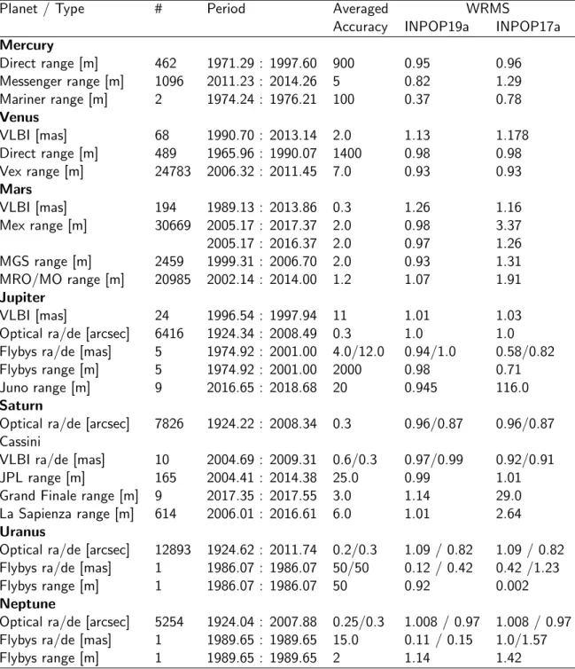
The full dataset used for the INPOP19a adjustment is presented in Tab 1.In this table are given the periods of each data sample as well as the number of observations and their average accuracies. The last two columns give the weighted root mean square (WRMS) for each data sample estimated with INPOP19a and INPOP17a.

2.1 Cassini independent data analysis

Refined Cassini’s normal points have been produced from a re-analysis of navigation data for the periods 2006, 2008-2009 and 2011. The new data analysis relies on the updated knowledge of the Saturnian system acquired throughout the mission: the enhanced accuracies achieved for Saturn’s moons ephemerides and the last gravity solutions of Saturn and its major satellites produced by the radio science team. The analysis shares the same concept of the navigation team’s reconstruction setup: trajectory arcs of approximately one month, spanning between two consecutive moons flybys (mainly Titan). For each arc we solve for the spacecraft initial position and velocity, corrections to orbital trim and reaction wheel desaturation maneuvers and RTG-induced anisotropic acceleration. In addition, stochastic accelerations at the level of 5 × 10−13 km/s2 (updated every 8 hours) are in-cluded to compensate for any remaining dynamical mismodeling. Considering the very good accuracy

Dec-01-2008 Feb-01-2009 Apr-01-2009 Jun-01-2009 Aug-01-2009 Oct-01-2009 Epoch -40.0 -20.0 0.0 20.0 40.0 60.0 80.0 100.0

Range bias (m, two-way)

T47 T48 T49 T50 T51 T52 T53 T54 T55 T56 T57 T58 T59T59 T60 T61 T62 E7 E8 0.0 20.0 40.0 60.0 80.0 100.0 120.0 140.0 160.0 180.0

SEP Angle (deg)

DSS 34 DSS 15 DSS 26 DSS 65 DSS 25 DSS 63 DSS 43 DSS 55 DSS 14 DSS 45 DSS 24 DSS 54 SEP angle

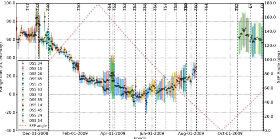
Figure 1: Estimated two-way range biases and formal uncertainties for the period 2008-2009. The annual trend is due to the residual error of INPOP17a ephemerides in the Earth-Saturn barycenter relative positioning.

obtained by [2] and [11] for the Titan and Saturn gravity fields, these latest were not adjusted in our analysis The dataset consists of two-way X-band Doppler and range data. We estimate correction to range measurements in the form of stochastic biases, different for each tracking pass, with large a priori uncertainty to absorb both station calibration and ephemerides error. In Fig ??are plotted the two-way range bias estimated over the period 2008:2009. The error bars were obtained by the projection of the least square covariance matrix on the line of sight.

The reconstructed Cassini trajectories are thus used to produce normal points, including the esti-mated range biases in the ground station-Cassini round-trip light-time computation. The uncertainty on the normal points is given be the estimated covariance matrix of range biases.

We have added also additional normal points deduced from the radio science solutions for the gravity-dedicated Titan flybys and Grand Finale Saturn pericenters. These range normal points were obtained in considering given spacecraft orbits constrained with only Doppler data for the Titan and Saturn gravity field estimations. By considering these supplementary normal points the period covered by the Cassini has been extended up to the end of 2017. In Tab. 1, the newly analysed normal points and the normal points deduced from Titan gravity flybys are labelled La Sapienza range when the data set deduced from the Grand Finale is labelled Grand Finale range.

2.2 Nine perijove of Juno

The Juno spacecraft is currently orbiting Jupiter in a highly eccentric, polar orbit since 2016. A radio-science experiment aims at characterizing the gravity field of the gas giant to unprecedented accuracy [6], [10]. Juno extremely accurate radio tracking system enables simultaneous two-way Doppler measurements at X- and Ka-band during the gravity-dedicated passes, which are used to reconstruct the spacecraft trajectory with mHz accuracies in the radial direction, at perijove. Range data points at X-band are collected as well, and Jovian barycenter positions relative to the Earth can be generated once per perijove pass, provided that we know Juno position with respect to the Jovian barycenter. In our fit, we include a total of 9 new Jupiter normal points spanning period from the orbital insertion, back in 2016, to end 2018.

3

Asteroid mass determination

As described in [3], we combine knowledge of the physical properties of asteroids by spatial or ground-based surveys, in particular spectral classes, to planetary ephemerides determinations of masses in order to enlarge the set of estimated asteroid masses and study their consistency with the spectral classes of the asteroids. For the mass determination, we use a constrained least square method based on the BVLS (Bounded Values Least Squares) algorithm from [13] which limits the fitted parameters to given intervals. Bounds have been selected according to the parameters of the fit: for asteroid masses, the lower bounds and the upper bounds are chosen according to the a priori masses and the a priori uncertainties deduced from the literature. The selection of 343 asteroids perturbing the planetary orbits is done based on the method of [12] and [7]. For defining the bounds, we separate the sample in the three taxonomic complexes C, S, and X according to the spectral informations extracted from the M3PC data base (mp3c.oca.eu). The spectra classes of asteroids can be grouped into the C-, S-, and X-complexes. For each asteroid, we estimate the smallest (lower bound) and the highest (upper bound) densities acceptable for these objects according to given uncertainties. The distribution of the lower bounds and of the upper bounds will constitute the prior distribution of the densities. In order to use the prior knowledge of the spectral complexes but in avoiding too strong constraints in the fit, we consider for each complex gaussian distributions of densities. Lower bounds values have been randomly selected in a (mean - 1σ) gaussian distribution when the upper bounds have been randomly selected in a (mean + 1σ) gaussian distribution. We then translate the density bounds into mass bounds as 4₃πD3_ρ

guess, i.e. assuming that the quoted D-values are spherical equivalent diameters.

A priori uncertainties on the initial guess values for the masses are also deduced by including the 3−σ diameter uncertainties to the density lower bounds and the upper bounds. A detailed description of the method is given in [3]. For each Monte Carlo runs, an iterative fit is performed in using the full planetary data sample (see Table 1). INPOP19a was selected among about 3600 adjustments, including the masses of the 343 perturber asteroids, performed for this study as the one minimizing the postfit residuals. Tab. 3gives the fitted masses of the 343 asteroids.

4

Trans-Neptunian Objects

In addition to the Main Belt objects described above (see section 3), the ten most massive TNO objects have been added to the list of planetary perturbers. As well as the Main Belt asteroids, their orbits are integrated together with the planets. A ring representing the average influence of TNO enclosed in the two main resonances with Neptune has been modeled in INPOP19a in considering 3 rings introduced by using point-mass bodies spread over three circular orbits located at 39.4, 44 and 47.5 AU. The sum of the mass of these three rings is estimated during the INPOP adjustment together with other parameters.. With the INPOP19a data sample including Juno and Cassini updated samples, we obtain for the TNO ring a mass of

Mring= (0.061 ± 0.001)ME.

If we limit the data sample to the sample used by [17], we obtain a mass of Mring= (0.020 ± 0.003)ME

consistent at 2-σ with the mass obtained by [17], considering the fact that the masses of the major TNO objects included in the modele are fixed in INPOP when they are fitted in [17]. So it is reasonable to think that the uncertainties of the fixed TNO masses in INPOP have been absorbed by the TNO ring mass, inducing a slightly bigger mass than the one obtained by [17]. We fixed the

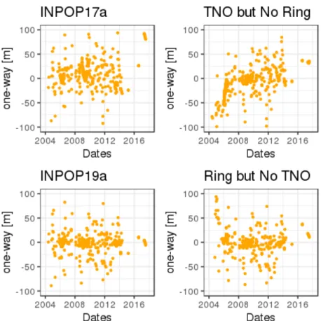
Figure 2: Saturn Postfit residuals obtained with INPOP17a (no ring, no TNO), INPOP19a (ring and TNO), one ephemeris including individual TNOs but no Ring (TNO but No Ring) and one ephemeris including a TNO ring but no individual TNOs (Ring but No TNO).

masses for the ten more massives TNO because these objects have at least one satellite and their masses are very accurately measured by the study of their satellites orbits (see Tab. 2).

The impact of the new modeling is clearly visible on the plots shown on Figure2. On these plots, one can see the Saturn postfit residuals deduced from the Cassini mission obtained with INPOP17a (with no ring and no individual TNOs) and with 3 differents modeles: one without individual TNO and TNO ring, one with individual TNO but no ring, one with both ring and individual TNO (INPOP19a). It appears clearly that the combined use of the 9 most massive TNOs together with the adjustment of the mass of a TNO ring improves significantly the postfit residuals, in particular if one considers an interval of time spread over several decades. With INPOP17a, the TNO accelerations were not required as the time span of the Cassini data was limited over almost 10 years (from 2004 to 2014). With the Grand Finale, the data sample has been extended over 13 years and INPOP17a clearly shows some trends (including bias) for the latest period (2017) that are not present when we include the full modeling including TNO individuals and ring .

5

INPOP accuracy

The global parameters of the INPOP19a ephemerides can be found in Tab. 3. This table is completed with the one (Tab. 10) of the 343 asteroids masses.

5.1 Postfit residuals

The last two columns of Table 1give the WRMS of the post-residuals obtained for INPOP19a and INPOP17a. As it can be seen the improvement is clear for Jupiter, Saturn and Mars.

For Mars, as explained in section 3 and in [3], the gain in postfit residuals is significant, in particular for the MRO/MO residuals which are the most accurate available data. In this case, INPOP19a improves INPOP17a residuals by 44% on a common interval of fit. For MEX, the extrapolation of INPOP17a out from its fitting interval (up to 2016.37) explains the more important dispersion of the residuals. However, even on its fitting interval, INPOP17a is less accurate than INPOP19a by 25 %.

For Jupiter the improvement is obviously brought by the Juno tracking data. It reaches 2 order of magnitude: from about 2 km for INPOP17a to 20 m for INPOP19a in keeping good residuals for the other flybys obtained between 1975 to 2001.

For Saturn, the prolongation of the data set from 2014 to 2017 was crucial to identify the contribution of TNOs into the perturbations to be applied on the Saturn orbit (see section 4). Furthermore the introduction of data obtained between 2006 and 2016 and analyzed independently from JPL (see section 2) is also very important to confirm that these data obtained in between 2006 and 2007 have to be taken into account in the adjustment with a high level of weighting. The improvement between INPOP17a and INPOP19a is of a factor 30 for the Grand Finale and 2.6 for the period between 2006 and 2016.

5.2 Propagation of the INPOP uncertainty

An interesting tool, especially for simulating future space missions, is to propagate with time the uncertainty obtained at J2000.

5.2.1 Mathematical formulation

INPOP is computed by solving numerically equations of motion. Let X(t) be the state vector in barycentric coordinates containing positions and velocities of each body which trajectory is computed. The numerical integrator solves a Cauchy-Lipschitz equations of motion system

dX

dt = F(X; P), X(t = J2000) = X0 (1)

where P ∈ Rp _{contains all the constant parameters of the ephemeris (initial conditions for the} planetary orbits, masses of the sun and of the asteroids including trans-Neptunian objects, oblateness of the sun, earth-moon mass ratio). Let us note that X and P are not independent variables because P includes the initial condition X0. Modification of P may modify X(t). From this ephemeris, we compute observational simulations in order to compare them to real data. Let C(ti, P) be the observation at date ticomputed with parameters P (we consider in what follows that the dependence with respect to X(ti) is included in the dependence with respect to the initial conditions included in P which are integrated by INPOP). The goal of the ephemeris is to minimize some norm of the residuals vector

R(ti, P) = (C(ti, P) − O(ti)) (2) where O(ti) is the real observation at date ti (for any matrix A, transpose of matrix A is noted tA). Usually, and this is what we do here, the linear Gaussian approximation is assumed and it is well known that the parameter s P which minimize χ2 =t_{RWR where W is the weigh matrix representing} the observational data accuracy, is given by the algorithm which increments P by iterations by adding

δP = −( t_J

until convergence is reached. Here, JC represents the Jacobian matrix of R(ti, P) or C(ti, P), which is computed numerically as follows

JC[i; k]= 1 2δk h C(ti, P1, . . . , Pk+ δk, . . . , Pp) − C(ti, P1, . . . , Pk−δk, . . . , Pp) i (4) Then it is well known that the covariance of P, which represents its uncertainty if the Gaussian and linear approximation are realized, is

cov P= ( tJW J)−1 (5)

From here, it is possible to propagate linearly the covariance of any variable computed with respect to the ephemeris and its parameters. Let H(t, P) ∈ Rh _{such a variable. Then for a linear} random Gaussian variation of P characterised by a covariance matrix covP, we can get the covariance of H at date t

cov H(t, P)= JH(t) covPtJH(t) (6) where JH(t) is the Jacobian matrix of H with respect to P at date t. To compute such a matrix, one needs to do the same procedure as for C(ti, P) which is formally equivalent.

In what follows, we will compute the linear covariance propagation of planetary RT N geocentric coordinates1 which are defined according to the following orthonormal basis for any planet A

uA = xA−xE MB |xA−xE MB| , (7) wA = uA× (vA−vE MB) |uA× (vA−vE MB)| , (8) vA = wA×uA (9)

where xA and represents the barycentric coordinates of body A, vA = dxA/dt, EMB label represents Earth-Moon barycenter, and × represents the vectorial product. Then we compute the quantities RA, TA, NA as follows

RA = (xA−xE MB) · uA (10)

TA = (xA−xE MB) · vA (11)

NA= (xA−xE MB) · wA (12)

From here we can deduce the propagated covariance of these three components on different bodies. It is interesting to compare the evolution of RTN components between two ephemerides. We can compare the difference between the components and the evolution of the covariance for two set of parameters P1 and P2 in order to compute a distance between two ephemerides. We can also do this for two different models, like INPOP17a and INPOP19a, in order to see if the difference between both is contained into the uncertainty ”tube” of the propagated covariance.

1_{Rigorously we should call it ”RTN Earh-Moon-barycenter coordinates” but no confusion is possible with the} following definitions.

5.2.2 Application to INPOP and results

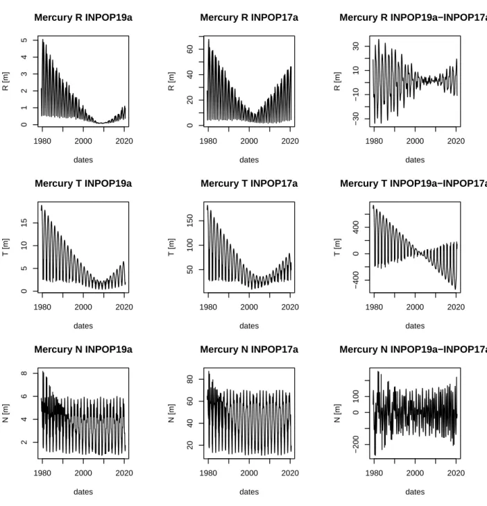
From Figures6to12are presented the propagations of the standard dispersion2 obtained at the end of the least square adjustment for INPOP19a and INPOP17a in RTN geocentric directions for the planets from Mercury to Neptune as well as the differences between the 2 ephemerides in geocentric RTN. The Figure 13 gives the propagation of the standard dispersion for the EMB orbit relative to the solar system barycenter (given in RTN barycentric). All propagation are given for a 40 years period, from 1980 to 2020.

In all the cases, INPOP19a shows lower propagated standard dispersion in comparison to IN-POP17a in all directions and even after 20 years of integration. For Mercury and Venus, the im-provement is about a factor 10 when it is of about a factor at least 4 (in R direction) and up to a factor 12 (in N direction) for Mars. For Jupiter, the improvement reaches a factor 50 in R and T directions when for Saturn as well as for Uranus and Neptune, the propagation of the INPOP19a standard dispersion is only 10 times better than the INPOP17a one. The differences between the ephemerides are consistent with the INPOP17a standard dispersion for the inner planets but are significantly greater for the outer planets. This can be explained by the introduction of the TNO in INPOP19a. As their contributions are mostly significant for the outer planet orbits and they were not considered in the INPO17a modeling, it is not surprising to have an underestimated uncertainty for INPOP17a for the outer planets. Finally for the EMB, the previous comments are also valid. However one can also note the important differences of the EMB orbit between INPOP19a and INPOP17a. These differences are explained at 97% by the contribution of the individual TNO and by 3% by the increase of 50% of the amount of main-belt asteroids (343 in INPOP19a compared to the 168 in INPOP17a) taken into account in the modelling. These massive bodies orbiting on non-perfectly circular orbits induce a displacement of the solar system barycenter that is visible in the differences of the EMB positions around the SSB between INPOP19a and INPOP17a. Finally it has to be stressed that these standard dispersion propagations are based on covariance matrices directly extracted from the least square adjustment. They give a good representation of the improvement between INPOP17a and INPOP19a. For more a realistic study of the INPOP19a uncertainties, other statistical tests have to be done.

5.3 Extrapolation Tests

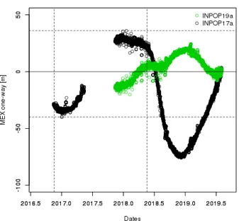
Finally, 18 months of MEX data has been put beside in order to test the INPOP19a extrapolation capabilities. On Figure 3 are presented the residuals obtained for INPOP19a and INPOP17a. IN-POP17a was fitted up to 2016.7 when INPOP19a was fitted on data up to 2017.37. Let us note the supplementary data interval used for the INPOP19a construction has an important gap, visible on Figure 3, due to the 2017 solar conjunction, leading to an effective supplementary interval of about 5 months. Nevertheless as one can see on Figure 3, the INPOP19a residuals are less impor-tant the one obtained with INPOP17a. Over the same interval of extrapolation (18 months), the INPOP19a residual dispersion decreases of about 50% in comparison to INPOP17a. If one considers the full interval, the extrapolation residuals are about about 3 times smaller for INPOP19a than for INPOP17a. This result shows the improvement of INPOP19a relative to INPOP17a in terms of Mars orbit extrapolation.

Figure 3: MEX one-way range extrapolation residuals (given in meters) obtained with INPOP17a (black) and INPOP19a (green). These residuals were obtained by comparisons between the ephemerides and observed distances not included in the data sample used for the fit. The dashed vertical lines indicate a 18-month period of extrapolation for INPOP17a and the dashed horizontal lines give the maximum and the minimum of the INPOP17a residuals for this 18-month extrapolation period.

6

Adjustment of asteroid orbit using GAIA DR2

6.1 Method

In 2013, was launched the astrometric satellite GAIA. Among observations of about 1 billion of stars with an accuracy down to 24 µarcseconds, the satellite also observed objects in the solar system. In 2018, were released positions and velocities of about 14 099 known Solar System objects mainly main belt, near Earth and Kuiper belt asteroids based on nearly 2 millions observations. The positions were acquired in the GAIA specific coordinates AL and AC as described in [9] with an optimal range of brightness G=12-17 where the accuracy in the AL-direction reaches milliarcsecond. As the error on AC remains considerably larger, the information provided by GAIA is essentially 1D. These particular features give rise to very strong correlations between right ascension and declination coordinates expressed in the barycentric reference system (BCRS) and have to be fully taken into account during the orbit determination process.

14099 orbits have then been integrated with INPOP together with the planetary and moon orbits. We fit these orbits to the GAIA data in using the correlation matrix provided by the DPAC. We did not fit the planetary orbits together with the asteroid orbits but we iterate the procedure in order to include the asteroid orbital improvements brought by the GAIA observations to the computation and the adjustment of the planet orbits (Mars mainly).

In order to integrate the motion of 14099 orbits in a reasonable time, we included the per-turbations of the Sun and of the main planets but in a newtonian formalism and in taking into account only a reduced number of the biggest asteroids that can have an influence on the other asteroid orbits. For a sake of comparison, we chose the same list of perturbing asteroids (16) as in [9]. However, after testing different alternative lists of perturbers, due to the limited interval of time covered by the GAIA data (22 months), no difference are noticeable on the residuals after the fit. For operating the inversion of such system (The size of the Jacobian matrix is 14099×6 × 1977702×2), a direct adjustment is very time consuming, This is why a strategy of block-wise algo-rithm has been set up using the Schur complement.

6.2 Asteroid orbit accuracy after fit

Fig. 4 presents the residuals obtained before and after the fit of the 14099 asteroids in using INPOP19a. The obtained results are very similar to those published to [9]. The mean and the standard deviation of the residuals after the adjustment is respectively 0.08 and 2.13 milliarcsecond in AL direction (compared to 0.05 and 2.14 in [9]). 96% of the AL residuals fall in the interval [-5,5] and 53% are at sub-milliarcsecond level. 98% of the AC residuals fall in the interval [-800 800]. 6.3 INPOP to Gaia reference frame tie

Because of the addition of 9 TNOs objects in INPOP19a, the position of the solar system barycenter has moved between INPOP19a and the ephemerides used for the definition of the GAIA SSB, IN-POP10e [4]. This can lead to a biased estimation of the GAIA spacecraft positions and consequently the asteroid observations. In order to take this offset into account, a constant translation on the GAIA barycentric position at J2000 (epoch of integration of the INPOP ephemerides) was fitted in the same time than asteroid orbit. The obtained value for the vector is x=-86.6, y=-49.3,z=-5.0 km. One can check that an equivalent displacement is obtained when comparing the barycentric EMB positions with respect to the solar system barycenter between INPOP17a (without TNO such as

Figure 4: Density plot of the residuals in the (AL,AC) plane expressed in milliarcsecond before and after the adjustement of the initial conditions. The colorbar and the axis range were chosen to be directly comparable with Fig.19 of [9]

INPOP10e) and INPOP19a.

In order to estimate the impact on the INPOP reference frame orientations of the use of the DR2 GAIA fitted asteroid orbits on the planet ones, we estimate a matrix of rotation between two planetary ephemerides differing only by the initial conditions of the orbits of the 343 asteroids taking into account for their perturbations on the planetary orbits.

The two ephemerides were fitted over the same data sample given in Table 1and in considering the same adjusted parameters. Same residuals have been obtained for the two solutions and no significant differences have been noticed in the fitted parameters, implying that the differences in the asteroid orbits are directly absorbed by the fitted parameters inside the estimated uncertainties.

This choice of fitting a rotation matrix between the two planetary ephemerides can be explained by the fact that the new asteroid orbits fitted over the Gaia DR2 are directly given in the Gaia reference frame ([8]) when the former asteroid orbits were given in a frame close to the one defined with the stellar catalogs such as USNOB1.1 and UCAC, leading to a tie to the ICRF2 with an accuracy of about several hundred of milli-arcseconds (mas) ([1]). This latest frame being at least two order of magnitude less accurate that the other data used for the planetary ephemerides tie to ICRF, when the two ephemerides are compared, we evaluate the rotation between the planetary orbits tied to ICRF with (delta DOR) observations of spacecraft orbiting planets ([5]) and planetary orbits adjusted using both ICRF VLBI positions of spacecraft and asteroid orbits given in the GRF. 3 Euler angles have been fitted and are given in Table4for different cases, depending which planetary orbits are considered. If all the orbits including the outer planet ones are considered, the mis-alignement of the INPOP reference frame axis (by definition, the ICRF , without considering the VLBI observation uncertainties) with the Gaia reference frame (GRF) is not significant. However if we consider only the orbits fitted over very accurate observations such as the inner planets, Jupiter and Saturn, then the Euler angles turn out to be significant but at the level of few µas. This is far below the uncertainty of the alignement between DR2 GRF and ICRF3 of about 20 to 30µas as obtained by ([8]). We can then conclude to a good alignement of the INPOP reference axis relative to the DR2 GRF.

7

Lunar ephemeris

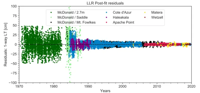
The lunar ephemeris of INPOP19a are obtained from the fit of the integrated solutions of the lunar orbit and orientation to the lunar laser ranging (LLR) data. The LLR data used for the fits of INPOP19a contains 27,780 normal points collected by eight Earth stations ranging to five lunar surface retroreflectors from August 1969 until October 2019. The LLR data is processed using the GINS software and the LLR reduction model is detailed in [22]. The dynamical model of the lunar interior is developed within INPOP19a following the description within [14,22]. Minor adjustments to the LLR data weights is made to benefit from the high accuracy of the LLR observations from APOLLO and Grasse stations. A total of 5725 infrared LLR observations collected between 2015-2019 were used for the fits of INPOP19a. The LLR data from the Wetzell station were retrieved from the POLAC and ILRS FTP websites for 2018 and 2019 data respectively. The comparison of LLR post-fit wrms obtained with INPOP17a and INPOP19a are provided in Table 5. We find that the wrms of the INPOP19a LLR post-fit residuals are very close to the 1 cm mark for Grasse, APOLLO and Wettzell stations.

The LLR fits of INPOP19a includes a supplementary correction to the longitude libration of the Moon (introduced within the GINS reduction software) to account for frequency dependence of lunar tidal dissipation. This introduces 3 cosine terms (l’, 2l-2D, 2F-2l) as corrections to the longitude libration of the Moon, similar to DE430 [25] and following the approximation in EPM2016 [15]. The cosine terms provide the out-of-phase component to the sine-dominated longitude libration terms (see for example the Fourier terms in the physical libration forτ tabulated in [18]). Introducing these

terms improves the LLR post-fit residuals by few mm (3-4 mm) visible more prominently over years 2010 to 2019, due to the higher accuracy of LLR data acquired during this period. The annual term (l’) has the most prominence among the three fitted amplitudes. Their values are tabulated in Table 7. We adapt this method for providing users with high accuracy requirements, until an equivalent dynamical model representation is introduced. Amplitudes of terms with longer periods (≥ 3yr) could in principle be fit at the current accuracy and long baseline of the data, but does not contribute to a significant improvement in the post-fit residuals.

Some of the parameters relevant to the Earth-Moon system are tabulated in Table 6. The differences in the gravitational mass of the Earth-Moon barycentre (GMEMB) arise from the use of updated values of the Earth-Moon mass ratio (EMRAT) provided by the joint iterative fit to the planetary part of the ephemeris. The INPOP17a solution reported a mean radial difference of ∼ 19 cm with respect to the last update of the JPL lunar solution (DE430) arising from the differences in GMEMB [22]. This difference is now reduced to ∼ 5 cm with the INPOP19a solution. Other differences in the lunar interior parameters are within their respective error bars. Few of the lunar gravity field coefficients (tabulated in Table 6) continue to require adjustment outside the error bar provided by the GRAIL gravity field solutions for a better fit of the LLR data. This is likely due to the simplicity of the forward modeling of the interior dynamics of the Moon as shown through recent efforts involving the joint analysis of GRAIL-LLR solutions [23]. The fluid core oblateness of the Moon (fc) differ by about 12% with respect to the INPOP17a solution for the same fixed core polar moment ratio as in INPOP17a (Cc

CT = 7×10

−4_{) and remains consistent with a recent in-house analysis} [21] involving an improved lunar interior paramaterization and a more complex torque modeling.

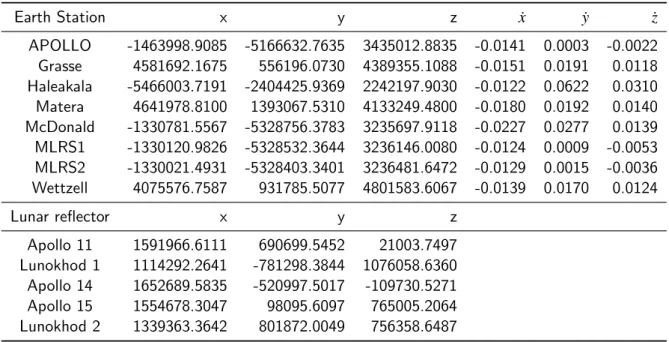
LLR data are not explicity used for ITRF solutions. However, some stations contribute other data products (GPS,SLR,VLBI) to the ITRF solutions. Stations with a long temporal baseline in LLR allow the fit of their coordinates (and in some cases, velocities) to the LLR data. Table 8 gives the list of station and reflector coordinates used for the INPOP19a solution. The INPOP17a document [19] contains a typographic error on reference values of the Lunokhod 1 and 2 reflector coordinates3. Users of the older INPOP17a solution must use their respective PA coordinates (XYZ in m) as L1XYZ=1114292.5047, -781298.2434, 1076058.5100 and L2XYZ=1339363.4749, 801872.1138, 756358.5308.

References

[1] Steven R. Chesley, James Baer, and David G. Monet. Treatment of star catalog biases in asteroid astrometric observations. Icarus, 210(1):158–181, Nov 2010.

[2] Daniele Durante, D. J. Hemingway, P. Racioppa, L. Iess, and D. J. Stevenson. Titan’s gravity field and interior structure after Cassini. Icarus, 326:123–132, Jul 2019.

[3] A. Fienga, C. Avdellidou, and J. Hanus. Asteroid masses obtained with inpop planetary ephemerides. ArXiv e-prints:1601.00947, 2019.

[4] A. Fienga, J. Laskar, H. Manche, M. Gastineau, and A. Verma. DPAC INPOP final release: INPOP10e. ArXiv e-prints , 2012.

[5] A. Fienga, J. Laskar, H. Manche, P. Kuchynka, G. Desvignes, M. Gastineau, I. Cognard, and G. Thereau. The planetary ephemerides INPOP10a and its applications in fundamental physics. Celest. Mech. Dyn. Astron., 111:363–+, 2011.

Table 1: INPOP19a data samples used for its adjustments. The columns 1 and 2 give the observed planet and an information on the space mission providing the observations. Columns 3 and 4 give the number of observations and the time interval, while the column 5gives the a priori uncertainties provided by space agencies or the navigation teams. Finally in the last two columns, are given the WRMS for INPOP19a and INPOP17a.

Planet / Type # Period Averaged WRMS

Accuracy INPOP19a INPOP17a Mercury Direct range [m] 462 1971.29 : 1997.60 900 0.95 0.96 Messenger range [m] 1096 2011.23 : 2014.26 5 0.82 1.29 Mariner range [m] 2 1974.24 : 1976.21 100 0.37 0.78 Venus VLBI [mas] 68 1990.70 : 2013.14 2.0 1.13 1.178 Direct range [m] 489 1965.96 : 1990.07 1400 0.98 0.98 Vex range [m] 24783 2006.32 : 2011.45 7.0 0.93 0.93 Mars VLBI [mas] 194 1989.13 : 2013.86 0.3 1.26 1.16 Mex range [m] 30669 2005.17 : 2017.37 2.0 0.98 3.37 2005.17 : 2016.37 2.0 0.97 1.26 MGS range [m] 2459 1999.31 : 2006.70 2.0 0.93 1.31 MRO/MO range [m] 20985 2002.14 : 2014.00 1.2 1.07 1.91 Jupiter VLBI [mas] 24 1996.54 : 1997.94 11 1.01 1.03

Optical ra/de [arcsec] 6416 1924.34 : 2008.49 0.3 1.0 1.0 Flybys ra/de [mas] 5 1974.92 : 2001.00 4.0/12.0 0.94/1.0 0.58/0.82 Flybys range [m] 5 1974.92 : 2001.00 2000 0.98 0.71 Juno range [m] 9 2016.65 : 2018.68 20 0.945 116.0 Saturn

Optical ra/de [arcsec] 7826 1924.22 : 2008.34 0.3 0.96/0.87 0.96/0.87 Cassini

VLBI ra/de [mas] 10 2004.69 : 2009.31 0.6/0.3 0.97/0.99 0.92/0.91 JPL range [m] 165 2004.41 : 2014.38 25.0 0.99 1.01 Grand Finale range [m] 9 2017.35 : 2017.55 3.0 1.14 29.0 La Sapienza range [m] 614 2006.01 : 2016.61 6.0 1.01 2.64 Uranus

Optical ra/de [arcsec] 12893 1924.62 : 2011.74 0.2/0.3 1.09 / 0.82 1.09 / 0.82 Flybys ra/de [mas] 1 1986.07 : 1986.07 50/50 0.12 / 0.42 0.42 /1.23 Flybys range [m] 1 1986.07 : 1986.07 50 0.92 0.002 Neptune

Optical ra/de [arcsec] 5254 1924.04 : 2007.88 0.25/0.3 1.008 / 0.97 1.008 / 0.97 Flybys ra/de [mas] 1 1989.65 : 1989.65 15.0 0.11 / 0.15 1.0/1.57 Flybys range [m] 1 1989.65 : 1989.65 2 1.14 1.42

1970 1980 1990 2000 2010 2020

Years

Residuals: 1-way LT [cm]

LLR Post-fit residuals

Figure 5: LLR post-fit residuals obtained with INPOP19a (wrms in cm) from 1969 to 2019.

TNO GM mass AU3d−2 kg 50000 7.235460e-14 4.863611e+20 55637 1.880380e-14 1.263975e+20 90482 9.554830e-14 6.422671e+20 120347 1.934696e-14 1.300485e+20 136108 6.036990e-13 4.058011e+21 136199 2.519160e-12 1.693357e+22 174567 3.994670e-14 2.685181e+20 208996 8.007340e-14 5.382462e+20 136472 4.498510e-13 3.023858e+21

Table 2: Masses for the nine biggest TNO kept fixed in INPOP19a. Values extracted from [17].

Table 3: Values of parameters obtained in the fit of INPOP13c, INPOP10e, DE430 and DE436 to observations.

INPOP13c INPOP17a INPOP19a DE436

± 1σ ± 1σ ± 1σ ± 1σ

(EMRAT-81.3000)× 10−4 _{(5.694 ± 0.010) ( 5.719 ± 0.010) (5.668 ± 0.010) 5.68217} J2× 10−7 (2.30 ± 0.25) (2.295 ± 0.010) (2.010 ± 0.010) NC GM - 132712440000 [km3. s−2] (44.487 ± 0.17) ( 42.693 ± 0.04) ( 40.042 ± 0.01) 41.939377

Table 4: Euler angles fitted by comparing two planet ephemerides different only by the asteroid orbits used for computing their perturbations on the planet orbits: one being fitted over the Gaia DR2 and one obtained from the astorb data base.

θ ψ φ

µas µas µas

All planets −98 ± 1508 1.0 ± 45 253 ± 3971

Inner planets 1.16 ± 0.20 −0.08 ± 0.62 −1.50 ± 0.150 Inner planets + Jupiter 1.23 ± 0.16 −1.0 ± 0.22 −0.128 ± 0.69 Inner planets + Jupiter + Saturn 1.83 ± 0.80 1.057 ± 0.053 −0.23 ± 2.56 Outer planets −55 ± 629 −30 ± 495 373 ± 5051

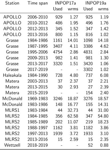
Table 5: Comparison of LLR post-fit residuals (wrms in cm) of LLR observations between INPOP17a (1969-2017) and INPOP19a (1969-2019). INPOP17a statistics are drawn from [20].

Station Time span INPOP17a INPOP19a Used wrms Used wrms APOLLO 2006-2010 929 1.27 925 1.19 APOLLO 2010-2012 486 1.95 496 1.76 APOLLO 2012-2013 345 1.52 347 1.42 APOLLO 2013-2016 800 1.15 816 1.02 Grasse 1984-1986 1161 14.01 1098 14.18 Grasse 1987-1995 3407 4.11 3386 4.62 Grasse 1995-2006 4754 2.86 4831 2.84 Grasse 2009-2013 982 1.41 981 1.30 Grasse 2013-2017 3320 1.51 3420 1.06 Grasse 2017-2019 - - 3302 1.02 Haleakala 1984-1990 728 4.80 737 6.08 Matera 2003-2013 37 2.37 37 2.21 Matera 2013-2015 30 2.93 27 2.39 Matera 2015-2019 - - 154 2.40 McDonald 1969-1983 3246 18.87 3276 18.57 McDonald 1983-1986 148 16.77 155 14.31 MLRS1 1983-1984 44 32.73 44 31.00 MLRS2 1984-1985 356 62.58 347 54.80 MLRS2 1985-1989 202 11.07 219 18.23 MLRS2 1988-1997 1162 3.81 1182 3.86 MLRS2 1997-2013 1939 3.72 1933 3.10 MLRS2 2013-2016 15 2.59 15 2.35 Wettzell 2018-2019 - - 52 0.88

Table 6: Parameters for the Earth-Moon system. Parameter Units INPOP17a INPOP19a

GMEMB au3/d2 8.997011404E-10 8.997011394E-10

τR1,E d 7.36E-03 7.98E-03

τR2,E d 2.89E-03 2.82E-03

CT/(MR2) 3.93148E-01 3.93140E-01 C32 4.84441E-06 4.84500E-06 S32 1.683E-06 1.685E-06 C33 1.6877E-06 1.6686E-06 τM d 8.7E-02 9.4E-02 kv/CT d−1 1.75E-08 1.64E-08 fc 2.5E-04 2.8E-04 h2 4.38E-02 4.26E-02

Table 7: Amplitudes of periodic terms as corrections to longitude librations (in mas) obtained be-tween ephemeris solutions to account for frequency-dependent dissipation in the Moon, where the polynomial expansion of the Delaunay arguments l’ (solar mean anomaly), l (lunar mean anomaly), F (argument of latitude) and D (mean elongation of the Moon from the Sun) follow Eqn. 5.43 in [16]. Columns labeled as DE430, WB2015, EPM2015 and EPM2017 were obtained from [7], [24], [15] and the IAA RAS website, respectively.

Parameter Period Longitude libration correction (in mas)

(d) DE430 WB2015 EPM2015 EPM2017 INPOP19a A1cos(l0) 365.26 5.0 ± 1.3 4.9 ± 1.1 4.5 ± 0.2 4.4 4.4 ± 0.6 A2cos(2l − 2D) 205.89 1.5 ± 1.2 2.0 ± 1.2 1.4 ± 0.2 1.6 1.7 ± 0.9 A₃cos(2F − 2l) 1095.22 -3.6 ± 3.3 0.7 ± 6.2 -7.3 ± 0.5 -5.2 9.7 ± 4.4

Table 8: Station and lunar surface reflector coordinates used for the fits of INPOP19a solution.

Earth Station x y z ˙x ˙y ˙z

APOLLO -1463998.9085 -5166632.7635 3435012.8835 -0.0141 0.0003 -0.0022 Grasse 4581692.1675 556196.0730 4389355.1088 -0.0151 0.0191 0.0118 Haleakala -5466003.7191 -2404425.9369 2242197.9030 -0.0122 0.0622 0.0310 Matera 4641978.8100 1393067.5310 4133249.4800 -0.0180 0.0192 0.0140 McDonald -1330781.5567 -5328756.3783 3235697.9118 -0.0227 0.0277 0.0139 MLRS1 -1330120.9826 -5328532.3644 3236146.0080 -0.0124 0.0009 -0.0053 MLRS2 -1330021.4931 -5328403.3401 3236481.6472 -0.0129 0.0015 -0.0036 Wettzell 4075576.7587 931785.5077 4801583.6067 -0.0139 0.0170 0.0124 Lunar reflector x y z Apollo 11 1591966.6111 690699.5452 21003.7497 Lunokhod 1 1114292.2641 -781298.3844 1076058.6360 Apollo 14 1652689.5835 -520997.5017 -109730.5271 Apollo 15 1554678.3047 98095.6097 765005.2064 Lunokhod 2 1339363.3642 801872.0049 756358.6487

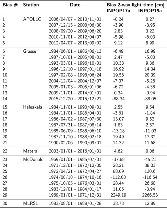
Table 9: Estimated values of station biases over different periods (2-way light time in cm). Bias # Station Date Bias 2-way light time [cm]

INPOP17a INPOP19a 1 APOLLO 2006/04/07 - 2010/11/01 -0.24 0.27 2 2007/12/15 - 2008/06/30 -3.90 -3.95 3 2008/09/20 - 2009/06/20 2.83 3.22 4 2010/11/01 - 2012/04/07 -5.98 -6.03 5 2012/04/07 - 2013/09/02 9.12 8.99 6 Grasse 1984/06/01 - 1986/06/13 -6.49 16.99 7 1987/10/01 - 2005/08/01 2.47 -5.00 8 1993/03/01 - 1996/10/01 10.38 9.36 9 1996/12/10 - 1997/01/18 16.92 14.04 10 1997/02/08 - 1998/06/24 19.56 20.39 11 2004/12/04 - 2004/12/07 -7.07 -5.28 12 2005/01/03 - 2005/01/06 -6.72 -4.38 13 2009/11/01 - 2014/01/01 0.34 -0.94 14 2015/12/20 - 2015/12/21 -88.34 -88.05 15 Haleakala 1984/11/01 - 1990/09/01 2.55 9.54 16 1984/11/01 - 1986/04/01 -3.61 -1.84 17 1986/04/02 - 1987/07/30 13.07 9.52 18 1987/07/31 - 1987/08/14 1.83 2.57 19 1985/06/09 - 1985/06/10 -13.18 -11.03 20 1987/11/10 - 1988/02/18 19.49 17.32 21 1990/02/06 - 1990/09/01 14.32 11.68 22 Matera 2003/01/01 - 2016/01/01 4.62 0.06 23 McDonald 1969/01/01 - 1985/07/01 -37.88 -45.21 24 1971/12/01 - 1972/12/05 28.21 38.03 25 1972/04/21 - 1972/04/27 88.09 130.6 26 1974/08/18 - 1974/10/16 -112.08 -116.54 27 1975/10/05 - 1976/03/01 28.44 26.68 28 1983/12/01 - 1984/01/17 11.06 -3.94 29 1969/01/01 - 1971/12/31 2249.19 2266.53 30 MLRS1 1983/08/01 - 1988/01/28 38.73 12.89

1980 2000 2020 0 1 2 3 4 5 Mercury R INPOP19a dates R [m] 1980 2000 2020 0 5 10 15 Mercury T INPOP19a dates T [m] 1980 2000 2020 2 4 6 8 Mercury N INPOP19a dates N [m] 1980 2000 2020 0 20 40 60 Mercury R INPOP17a dates R [m] 1980 2000 2020 50 100 150 Mercury T INPOP17a dates T [m] 1980 2000 2020 20 40 60 80 Mercury N INPOP17a dates N [m] 1980 2000 2020 −30 −10 10 30 Mercury R INPOP19a−INPOP17a dates R [m] 1980 2000 2020 −400 0 400 Mercury T INPOP19a−INPOP17a dates T [m] 1980 2000 2020 −200 0 100 Mercury N INPOP19a−INPOP17a dates N [m]

Figure 6: Propagation of least squares standard dispersion for the orbit of Mercury in the case of INPOP19a and INPOP17a. Right-hand side plots give the geocentric differences for Mercury (INPOP19a-INPOP17a) integrated positions. All the differences and Propagation of least squares standard dispersion are given in (R,T,N) geocentric frame.

1980 2000 2020 0 1 2 3 4 5 6 7 Venus R INPOP19a dates R [m] 1980 2000 2020 5 10 15 Venus T INPOP19a dates T [m] 1980 2000 2020 2 4 6 8 10 12 Venus N INPOP19a dates N [m] 1980 2000 2020 0 20 60 100 Venus R INPOP17a dates R [m] 1980 2000 2020 50 100 150 Venus T INPOP17a dates T [m] 1980 2000 2020 20 40 60 80 120 Venus N INPOP17a dates N [m] 1980 2000 2020 −60 −20 20 60 Venus R INPOP19a−INPOP17a dates R [m] 1980 2000 2020 −400 0 400 Venus T INPOP19a−INPOP17a dates T [m] 1980 2000 2020 −400 0 200 400 Venus N INPOP19a−INPOP17a dates N [m]

Figure 7: Propagation of least squares standard dispersion for the orbit of Venus in the case of IN-POP19a and INPOP17a. Right-hand side plots give the geocentric differences for Venus (ININ-POP19a- (INPOP19a-INPOP17a) integrated positions. All the differences and propagation of least squares standard dis-persion are given in (R,T,N) geocentric frame.

1980 2000 2020 0 20 40 60 80 Mars R INPOP19a dates R [m] 1980 2000 2020 0 20 60 100 140 Mars T INPOP19a dates T [m] 1980 2000 2020 2 4 6 8 10 Mars N INPOP19a dates N [m] 1980 2000 2020 0 100 300 500 Mars R INPOP17a dates R [m] 1980 2000 2020 0 200 400 600 Mars T INPOP17a dates T [m] 1980 2000 2020 20 40 60 80 100 120 Mars N INPOP17a dates N [m] 1980 2000 2020 −500 0 500 Mars R INPOP19a−INPOP17a dates R [m] 1980 2000 2020 −800 −400 0 200 Mars T INPOP19a−INPOP17a dates T [m] 1980 2000 2020 −200 0 100 200 Mars N INPOP19a−INPOP17a dates N [m]

Figure 8: Propagation of least squares standard dispersion for the orbit of Mars in the case of IN-POP19a and INPOP17a. Right-hand side plots give the geocentric differences for Mars (ININ-POP19a- (INPOP19a-INPOP17a) integrated positions. All the differences and propagation of least squares standard dis-persion are given in (R,T,N) geocentric frame for Mars and (R,T,N) barycentric frame for EMB.

1980 2000 2020 0 5 10 20 30 Jupiter INPOP19a dates R [m] 1980 2000 2020 20 40 60 80 dates T [m] 1980 2000 2020 65 70 75 80 85 90 dates N [m] 1980 2000 2020 200 600 1000 1400 Jupiter INPOP17a dates R [m] 1980 2000 2020 1000 2000 3000 4000 dates T [m] 1980 2000 2020 1000 2000 3000 dates N [m] 1980 2000 2020 −2000 0 2000 Jupiter INPOP19a−INPOP17a dates R [m] 1980 2000 2020 −10000 −5000 0 5000 dates T [m] 1980 2000 2020 −20000 0 10000 dates N [m]

Figure 9: Propagation of least squares standard dispersion for the orbit of Jupiter in the case of INPOP19a and INPOP17a. Right-hand side plots give the geocentric differences for Jupiter (INPOP19a-INPOP17a) integrated positions. All the differences and propagation of least squares standard dispersion are given in (R,T,N) geocentric frame.

1980 2000 2020 0 5 10 15 20 Saturn R INPOP19a dates R [m] 1980 2000 2020 20 40 60 80 100 Saturn T INPOP19a dates T [m] 1980 2000 2020 20 25 30 35 40 Saturn N INPOP19a dates N [m] 1980 2000 2020 50 100 150 200 250 Saturn R INPOP17a dates R [m] 1980 2000 2020 200 400 600 800 1200 Saturn T INPOP17a dates T [m] 1980 2000 2020 400 450 500 Saturn N INPOP17a dates N [m] 1980 2000 2020 −500 0 500 1000 Saturn R INPOP19a−INPOP17a dates R [m] 1980 2000 2020 −2000 0 2000 4000 Saturn T INPOP19a−INPOP17a dates T [m] 1980 2000 2020 −3000 −1000 1000 3000 Saturn N INPOP19a−INPOP17a dates N [m]

Figure 10: Propagation of least squares standard dispersion for the orbit of Saturn in the case of INPOP19a and INPOP17a. Right-hand side plots give the geocentric differences for Saturn (INPOP19a-INPOP17a) integrated positions. All the differences and propagation of least squares standard dispersion are given in (R,T,N) geocentric frame.

1980 2000 2020 0 5 10 15 20 25 30 Uranus R INPOP19a dates R [km] 1980 2000 2020 10 20 30 40 Uranus T INPOP19a dates T [km] 1980 2000 2020 6 8 10 12 Uranus N INPOP19a dates N [km] 1980 2000 2020 0 100 200 300 400 Uranus R INPOP17a dates R [km] 1980 2000 2020 200 400 600 800 Uranus T INPOP17a dates T [km] 1980 2000 2020 150 200 250 300 350 Uranus N INPOP17a dates N [km] 1980 2000 2020 0 200 400 600 800 Uranus R INPOP19a−INPOP17a dates R [km] 1980 2000 2020 −1500 −1000 −500 Uranus T INPOP19a−INPOP17a dates T [km] 1980 2000 2020 −500 0 500 Uranus N INPOP19a−INPOP17a dates N [km]

Figure 11: Propagation of least squares standard dispersion for the orbit of Uranus in the case of INPOP19a and INPOP17a. Right-hand side plots give the geocentric differences for Uranus (INPOP19a-INPOP17a) integrated positions. All the differences and propagation of least squares standard dispersion are given in (R,T,N) geocentric frame.

1980 2000 2020 0 50 100 150 Neptune R INPOP19a dates R [km] 1980 2000 2020 10 30 50 70 Neptune T INPOP19a dates T [km] 1980 2000 2020 10 15 20 25 30 Neptune N INPOP19a dates N [km] 1980 2000 2020 0 500 1500 2500 Neptune R INPOP17a dates R [km] 1980 2000 2020 400 800 1200 Neptune T INPOP17a dates T [km] 1980 2000 2020 400 500 600 700 800 Neptune N INPOP17a dates N [km] 1980 2000 2020 −3000 −1000 0 Neptune R INPOP19a−INPOP17a dates R [km] 1980 2000 2020 −500 0 500 1000 Neptune T INPOP19a−INPOP17a dates T [km] 1980 2000 2020 −500 −450 −400 −350 Neptune N INPOP19a−INPOP17a dates N [km]

Figure 12: Propagation of least squares standard dispersion for the orbit of Neptune in the case of INPOP19a and INPOP17a. Right-hand side plots give the geocentric differences for Neptune (INPOP19a-INPOP17a) integrated positions. All the differences and propagation of least squares standard dispersion are given in (R,T,N) geocentric frame.

1980 2000 2020 0 50 100 150 EMB R INPOP19a dates R [km] 1980 2000 2020 10 30 50 70 EMB T INPOP19a dates T [km] 1980 2000 2020 10 15 20 25 30 EMB N INPOP19a dates N [km] 1980 2000 2020 0 200 600 1000 EMB R INPOP17a dates R [km] 1980 2000 2020 0 200 600 1000 EMB T INPOP17a dates T [km] 1980 2000 2020 40 50 60 70 80 90 EMB N INPOP17a dates N [km] 1980 2000 2020 −30 −10 0 10 20 EMB R INPOP19a−INPOP17a dates R [km] 1980 2000 2020 −10 −5 0 5 10 EMB T INPOP19a−INPOP17a dates T [km] 1980 2000 2020 −100 −50 0 50 EMB N INPOP19a−INPOP17a dates N [km]

Figure 13: Propagation of least squares standard dispersion for the orbit of EMB versus SSB in the case of INPOP19a and INPOP17a. Right-hand side plots give the SSB differences for EMB (INPOP19a-INPOP17a) integrated positions. All the differences and propagation of least squares standard dispersion are given in (R,T,N) barycentric frame.

[6] W. M. Folkner, L. Iess, J. D. Anderson, S. W. Asmar, D. R. Buccino, D. Durante, M. Feldman, L. Gomez Casajus, M. Gregnanin, A. Milani, M. Parisi, R. S. Park, D. Serra, G. Tommei, P. Tortora, M. Zannoni, S. J. Bolton, J. E. P. Connerney, and S. M. Levin. Jupiter gravity field estimated from the first two juno orbits. Geophysical Research Letters, 44(10):4694–4700, 2017.

[7] W. M. Folkner, J. G. Williams, D. H. Boggs, R. S. Park, and P. Kuchynka. The Planetary and Lunar Ephemerides DE430 and DE431. Interplanetary Network Progress Report, 196:C1, February 2014.

[8] Gaia Collaboration, Mignard, F., Klioner, S. A., Lindegren, L., Hern´andez, J., Bastian, U., Bom-brun, A., Hobbs, D., Lammers, U., Michalik, D., Ramos-Lerate, M., Biermann, M., Fern´ andez-Hern´andez, J., Geyer, R., Hilger, T., Siddiqui, H. I., Steidelm¨uller, H., Babusiaux, C., Barache, C., Lambert, S., Andrei, A. H., Bourda, G., Charlot, P., Brown, A. G. A., Vallenari, A., Prusti, T., de Bruijne, J. H. J., Bailer-Jones, C. A. L., Evans, D. W., Eyer, L., Jansen, F., Jordi, C., Luri, X., Panem, C., Pourbaix, D., Randich, S., Sartoretti, P., Soubiran, C., van Leeuwen, F., Walton, N. A., Arenou, F., Cropper, M., Drimmel, R., Katz, D., Lattanzi, M. G., Bakker, J., Cacciari, C., Casta˜neda, J., Chaoul, L., Cheek, N., De Angeli, F., Fabricius, C., Guerra, R., Holl, B., Masana, E., Messineo, R., Mowlavi, N., Nienartowicz, K., Panuzzo, P., Portell, J., Riello, M., Seabroke, G. M., Tanga, P., Th´evenin, F., Gracia-Abril, G., Comoretto, G., Garcia-Reinaldos, M., Teyssier, D., Altmann, M., Andrae, R., Audard, M., Bellas-Velidis, I., Benson, K., Berthier, J., Blomme, R., Burgess, P., Busso, G., Carry, B., Cellino, A., Clemen-tini, G., Clotet, M., Creevey, O., Davidson, M., De Ridder, J., Delchambre, L., Dell´Oro, A., Ducourant, C., Fouesneau, M., Fr´emat, Y., Galluccio, L., Garc´ıa-Torres, M., Gonz´alez-N´u˜nez, J., Gonz´alez-Vidal, J. J., Gosset, E., Guy, L. P., Halbwachs, J.-L., Hambly, N. C., Harrison, D. L., Hestroffer, D., Hodgkin, S. T., Hutton, A., Jasniewicz, G., Jean-Antoine-Piccolo, A., Jor-dan, S., Korn, A. J., Krone-Martins, A., Lanzafame, A. C., Lebzelter, T., L¨offler, W., Manteiga, M., Marrese, P. M., Mart´ın-Fleitas, J. M., Moitinho, A., Mora, A., Muinonen, K., Osinde, J., Pancino, E., Pauwels, T., Petit, J.-M., Recio-Blanco, A., Richards, P. J., Rimoldini, L., Robin, A. C., Sarro, L. M., Siopis, C., Smith, M., Sozzetti, A., S¨uveges, M., Torra, J., van Reeven, W., Abbas, U., Abreu Aramburu, A., Accart, S., Aerts, C., Altavilla, G., ´Alvarez, M. A., Alvarez, R., Alves, J., Anderson, R. I., Anglada Varela, E., Antiche, E., Antoja, T., Arcay, B., Astraat-madja, T. L., Bach, N., Baker, S. G., Balaguer-N´u˜nez, L., Balm, P., Barata, C., Barbato, D., Barblan, F., Barklem, P. S., Barrado, D., Barros, M., Barstow, M. A., Bartholom´e Mu˜noz, L., Bassilana, J.-L., Becciani, U., Bellazzini, M., Berihuete, A., Bertone, S., Bianchi, L., Bienaym´e, O., Blanco-Cuaresma, S., Boch, T., Boeche, C., Borrachero, R., Bossini, D., Bouquillon, S., Bragaglia, A., Bramante, L., Breddels, M. A., Bressan, A., Brouillet, N., Br¨usemeister, T., Brugaletta, E., Bucciarelli, B., Burlacu, A., Busonero, D., Butkevich, A. G., Buzzi, R., Caffau, E., Cancelliere, R., Cannizzaro, G., Cantat-Gaudin, T., Carballo, R., Carlucci, T., Carrasco, J. M., Casamiquela, L., Castellani, M., Castro-Ginard, A., Chemin, L., Chiavassa, A., Cocozza, G., Costigan, G., Cowell, S., Crifo, F., Crosta, M., Crowley, C., Cuypers, J., Dafonte, C., Damerdji, Y., Dapergolas, A., David, P., David, M., de Laverny, P., De Luise, F., De March, R., de Souza, R., de Torres, A., Debosscher, J., del Pozo, E., Delbo, M., Delgado, A., Delgado, H. E., Diakite, S., Diener, C., Distefano, E., Dolding, C., Drazinos, P., Dur´an, J., Edvardsson, B., Enke, H., Eriksson, K., Esquej, P., Eynard Bontemps, G., Fabre, C., Fabrizio, M., Faigler, S., Falc˜ao, A. J., Farr`as Casas, M., Federici, L., Fedorets, G., Fernique, P., Figueras, F., Filippi, F., Findeisen, K., Fonti, A., Fraile, E., Fraser, M., Fr´ezouls, B., Gai, M., Galleti, S., Garabato, D., Garc´ıa-Sedano, F., Garofalo, A., Garralda, N., Gavel, A., Gavras, P., Gerssen, J., Giacobbe, P., Gilmore, G., Girona, S., Giuffrida, G., Glass, F., Gomes, M., Granvik, M., Gueguen, A., Guerrier, A., Guiraud, J., Guti´e, R., Haigron, R., Hatzidimitriou, D., Hauser, M., Haywood, M., Heiter,

U., Helmi, A., Heu, J., Hofmann, W., Holland, G., Huckle, H. E., Hypki, A., Icardi, V., Janßen, K., Jevardat de Fombelle, G., Jonker, P. G., Juh´asz, A. L., Julbe, F., Karampelas, A., Kewley, A., Klar, J., Kochoska, A., Kohley, R., Kolenberg, K., Kontizas, M., Kontizas, E., Koposov, S. E., Kordopatis, G., Kostrzewa-Rutkowska, Z., Koubsky, P., Lanza, A. F., Lasne, Y., Lavigne, J.-B., Le Fustec, Y., Le Poncin-Lafitte, C., Lebreton, Y., Leccia, S., Leclerc, N., Lecoeur-Taibi, I., Lenhardt, H., Leroux, F., Liao, S., Licata, E., Lindstrøm, H. E. P., Lister, T. A., Livanou, E., Lobel, A., L´opez, M., Managau, S., Mann, R. G., Mantelet, G., Marchal, O., Marchant, J. M., Marconi, M., Marinoni, S., Marschalk´o, G., Marshall, D. J., Martino, M., Marton, G., Mary, N., Massari, D., Matijevic, G., Mazeh, T., McMillan, P. J., Messina, S., Millar, N. R., Molina, D., Molinaro, R., Moln´ar, L., Montegriffo, P., Mor, R., Morbidelli, R., Morel, T., Morris, D., Mulone, A. F., Muraveva, T., Musella, I., Nelemans, G., Nicastro, L., Noval, L., O´Mullane, W., Ord´enovic, C., Ord´o˜nez-Blanco, D., Osborne, P., Pagani, C., Pagano, I., Pailler, F., Palacin, H., Palaversa, L., Panahi, A., Pawlak, M., Piersimoni, A. M., Pineau, F.-X., Plachy, E., Plum, G., Poggio, E., Poujoulet, E., Prsa, A., Pulone, L., Racero, E., Ragaini, S., Rambaux, N., Regibo, S., Reyl´e, C., Riclet, F., Ripepi, V., Riva, A., Rivard, A., Rixon, G., Roegiers, T., Roelens, M., Romero-G´omez, M., Rowell, N., Royer, F., Ruiz-Dern, L., Sadowski, G., Sagrist`a Sell´es, T., Sahlmann, J., Salgado, J., Salguero, E., Sanna, N., Santana-Ros, T., Sarasso, M., Savietto, H., Schultheis, M., Sciacca, E., Segol, M., Segovia, J. C., S´egransan, D., Shih, I.-C., Siltala, L., Silva, A. F., Smart, R. L., Smith, K. W., Solano, E., Solitro, F., Sordo, R., Soria Nieto, S., Souchay, J., Spagna, A., Spoto, F., Stampa, U., Steele, I. A., Stephenson, C. A., Stoev, H., Suess, F. F., Surdej, J., Szabados, L., Szegedi-Elek, E., Tapiador, D., Taris, F., Tauran, G., Taylor, M. B., Teixeira, R., Terrett, D., Teyssandier, P., Thuillot, W., Titarenko, A., Torra Clotet, F., Turon, C., Ulla, A., Utrilla, E., Uzzi, S., Vaillant, M., Valentini, G., Valette, V., van Elteren, A., Van Hemelryck, E., van Leeuwen, M., Vaschetto, M., Vecchiato, A., Veljanoski, J., Viala, Y., Vicente, D., Vogt, S., von Essen, C., Voss, H., Votruba, V., Voutsinas, S., Walmsley, G., Weiler, M., Wertz, O., Wevers, T., Wyrzykowski, L., Yoldas, A., Zerjal, M., Ziaeepour, H., Zorec, J., Zschocke, S., Zucker, S., Zurbach, C., and Zwitter, T. Gaia data release 2 - the celestial reference frame (gaia-crf2). A&A, 616:A14, 2018.

[9] Gaia Collaboration, F. Spoto, P. Tanga, F. Mignard, J. Berthier, B. Carry, A. Cellino, A. Dell’Oro, D. Hestroffer, K. Muinonen, T. Pauwels, J. M. Petit, P. David, F. De Angeli, M. Delbo, B. Fr´ezouls, L. Galluccio, M. Granvik, J. Guiraud, J. Hern´andez, C. Ord´enovic, J. Portell, E. Poujoulet, W. Thuillot, G. Walmsley, A. G. A. Brown, A. Vallenari, T. Prusti, J. H. J. de Bruijne, C. Babusiaux, C. A. L. Bailer-Jones, M. Biermann, D. W. Evans, L. Eyer, F. Jansen, C. Jordi, S. A. Klioner, U. Lammers, L. Lindegren, X. Luri, C. Panem, D. Pourbaix, S. Randich, P. Sartoretti, H. I. Siddiqui, C. Soubiran, F. van Leeuwen, N. A. Walton, F. Are-nou, U. Bastian, M. Cropper, R. Drimmel, D. Katz, M. G. Lattanzi, J. Bakker, C. Cacciari, J. Casta˜neda, L. Chaoul, N. Cheek, C. Fabricius, R. Guerra, B. Holl, E. Masana, R. Messineo, N. Mowlavi, K. Nienartowicz, P. Panuzzo, M. Riello, G. M. Seabroke, F. Th´evenin, G. Gracia-Abril, G. Comoretto, M. Garcia-Reinaldos, D. Teyssier, M. Altmann, R. Andrae, M. Audard, I. Bellas-Velidis, K. Benson, R. Blomme, P. Burgess, G. Busso, G. Clementini, M. Clotet, O. Creevey, M. Davidson, J. De Ridder, L. Delchambre, C. Ducourant, J. Fern´andez-Hern´andez, M. Fouesneau, Y. Fr´emat, M. Garc´ıa-Torres, J. Gonz´alez-N´u˜nez, J. J. Gonz´alez-Vidal, E. Gosset, L. P. Guy, J. L. Halbwachs, N. C. Hambly, D. L. Harrison, S. T. Hodgkin, A. Hutton, G. Jas-niewicz, A. Jean-Antoine-Piccolo, S. Jordan, A. J. Korn, A. Krone-Martins, A. C. Lanzafame, T. Lebzelter, W. L¨o, M. Manteiga, P. M. Marrese, J. M. Mart´ın-Fleitas, A. Moitinho, A. Mora, J. Osinde, E. Pancino, A. Recio-Blanco, P. J. Richards, L. Rimoldini, A. C. Robin, L. M. Sarro, C. Siopis, M. Smith, A. Sozzetti, M. S¨uveges, J. Torra, W. van Reeven, U. Abbas, A. Abreu Aramburu, S. Accart, C. Aerts, G. Altavilla, M. A. ´Alvarez, R. Alvarez, J. Alves, R. I. Anderson,

A. H. Andrei, E. Anglada Varela, E. Antiche, T. Antoja, B. Arcay, T. L. Astraatmadja, N. Bach, S. G. Baker, L. Balaguer-N´u˜nez, P. Balm, C. Barache, C. Barata, D. Barbato, F. Barblan, P. S. Barklem, D. Barrado, M. Barros, M. A. Barstow, L. Bartholom´e Mu˜noz, J. L. Bassilana, U. Bec-ciani, M. Bellazzini, A. Berihuete, S. Bertone, L. Bianchi, O. Bienaym´e, S. Blanco-Cuaresma, T. Boch, C. Boeche, A. Bombrun, R. Borrachero, D. Bossini, S. Bouquillon, G. Bourda, A. Bra-gaglia, L. Bramante, M. A. Breddels, A. Bressan, N. Brouillet, T. Br¨usemeister, E. Brugaletta, B. Bucciarelli, A. Burlacu, D. Busonero, A. G. Butkevich, R. Buzzi, E. Caffau, R. Cancelliere, G. Cannizzaro, T. Cantat-Gaudin, R. Carballo, T. Carlucci, J. M. Carrasco, L. Casamiquela, M. Castellani, A. Castro-Ginard, P. Charlot, L. Chemin, A. Chiavassa, G. Cocozza, G. Costigan, S. Cowell, F. Crifo, M. Crosta, C. Crowley, J. Cuypers, C. Dafonte, Y. Damerdji, A. Dapergolas, M. David, P. de Laverny, F. De Luise, R. De March, R. de Souza, A. de Torres, J. Debosscher, E. del Pozo, A. Delgado, H. E. Delgado, S. Diakite, C. Diener, E. Distefano, C. Dolding, P. Drazi-nos, J. Dur´an, B. Edvardsson, H. Enke, K. Eriksson, P. Esquej, G. Eynard Bontemps, C. Fabre, M. Fabrizio, S. Faigler, A. J. Falc˜ao, M. Farr`as Casas, L. Federici, G. Fedorets, P. Fernique, F. Figueras, F. Filippi, K. Findeisen, A. Fonti, E. Fraile, M. Fraser, M. Gai, S. Galleti, D. Gara-bato, F. Garc´ıa-Sedano, A. Garofalo, N. Garralda, A. Gavel, P. Gavras, J. Gerssen, R. Geyer, P. Giacobbe, G. Gilmore, S. Girona, G. Giuffrida, F. Glass, M. Gomes, A. Gueguen, A. Guerrier, R. Guti´e, R. Haigron, D. Hatzidimitriou, M. Hauser, M. Haywood, U. Heiter, A. Helmi, J. Heu, T. Hilger, D. Hobbs, W. Hofmann, G. Holland , H. E. Huckle, A. Hypki, V. Icardi, K. Janßen, G. Jevardat de Fombelle, P. G. Jonker, ´A. L. Juh´asz, F. Julbe, A. Karampelas, A. Kewley, J. Klar, A. Kochoska, R. Kohley, K. Kolenberg, M. Kontizas, E. Kontizas, S. E. Koposov, G. Kordopatis, Z. Kostrzewa-Rutkowska, P. Koubsky, S. Lambert, A. F. Lanza, Y. Lasne, J. B. Lavigne, Y. Le Fustec, C. Le Poncin-Lafitte, Y. Lebreton, S. Leccia, N. Leclerc, I. Lecoeur-Taibi, H. Lenhardt, F. Leroux, S. Liao, E. Licata, H. E. P. Lindstrøm, T. A. Lister, E. Livanou, A. Lobel, M. L´opez, S. Managau, R. G. Mann, G. Mantelet, O. Marchal, J. M. Marchant, M. Marconi, S. Marinoni, G. Marschalk´o, D. J. Marshall, M. Martino, G. Marton, N. Mary, D. Massari, G. Matijeviˇc, T. Mazeh, P. J. McMillan, S. Messina, D. Michalik, N. R. Millar, D. Molina, R. Molinaro, L. Moln´ar, P. Montegriffo, R. Mor, R. Morbidelli, T. Morel, D. Morris, A. F. Mulone, T. Muraveva, I. Musella, G. Nelemans, L. Nicastro, L. Noval, W. O’Mullane, D. Ord´o˜nez-Blanco, P. Osborne, C. Pagani, I. Pagano, F. Pailler, H. Palacin, L. Palaversa, A. Panahi, M. Pawlak, A. M. Piersimoni, F. X. Pineau, E. Plachy, G. Plum, E. Poggio, A. Prˇsa, L. Pulone, E. Racero, S. Ragaini, N. Rambaux, M. Ramos-Lerate, S. Regibo, C. Reyl´e, F. Ri-clet, V. Ripepi, A. Riva, A. Rivard, G. Rixon, T. Roegiers, M. Roelens, M. Romero-G´omez, N. Rowell, F. Royer, L. Ruiz-Dern, G. Sadowski, T. Sagrist`a Sell´es, J. Sahlmann, J. Salgado, E. Salguero, N. Sanna, T. Santana-Ros, M. Sarasso, H. Savietto, M. Schultheis, E. Sciacca, M. Segol, J. C. Segovia, D. S´egransan, I. C. Shih, L. Siltala, A. F. Silva, R. L. Smart, K. W. Smith, E. Solano, F. Solitro, R. Sordo, S. Soria Nieto, J. Souchay, A. Spagna, U. Stampa, I. A. Steele, H. Steidelm¨uller, C. A. Stephenson, H. Stoev, F. F. Suess, J. Surdej, L. Szaba-dos, E. Szegedi-Elek, D. Tapiador, F. Taris, G. Tauran, M. B. Taylor, R. Teixeira, D. Terrett, P. Teyssand ier, A. Titarenko, F. Torra Clotet, C. Turon, A. Ulla, E. Utrilla, S. Uzzi, M. Vaillant, G. Valentini, V. Valette, A. van Elteren, E. Van Hemelryck, M. van Leeuwen, M. Vaschetto, A. Vecchiato, J. Veljanoski, Y. Viala, D. Vicente, S. Vogt, C. von Essen, H. Voss, V. Votruba, S. Voutsinas, M. Weiler, O. Wertz, T. Wevers, . Wyrzykowski, A. Yoldas, M. ˇZerjal, H. Zi-aeepour, J. Zorec, S. Zschocke, S. Zucker, C. Zurbach, and T. Zwitter. Gaia Data Release 2. Observations of solar system objects. A&A, 616:A13, Aug 2018.

[10] L. Iess, W. M. Folkner, D. Durante, M. Parisi, Y. Kaspi, E. Galanti, T. Guillot, W. B. Hub-bard, D. J. Stevenson, J. D. Anderson, D. R. Buccino, L. Gomez Casajus, A. Milani, R. Park, P. Racioppa, D. Serra, P. Tortora, M. Zannoni, H. Cao, R. Helled, J. I. Lunine, Y. Miguel,

B. Militzer, S. Wahl, J. E. P. Connerney, S. M. Levin, and S. J. Bolton. Measurement of jupiter’s asymmetric gravity field. Nature, 555:220 EP –, 03 2018.

[11] L. Iess, B. Militzer, Y. Kaspi, P. Nicholson, D. Durante, P. Racioppa, A. Anabtawi, E. Galanti, W. Hubbard, M. J. Mariani, P. Tortora, S. Wahl, and M. Zannoni. Measurement and implications of saturn’s gravity field and ring mass. Science, 364(6445), 2019.

[12] P. Kuchynka and W. M. Folkner. A new approach to determining asteroid masses from planetary range measurements. Icarus, 222:243–253, January 2013.

[13] C. Lawson and R. Hanson. Solving least squares problems. SIAM, 1974. [14] Herv´e Manche. PhD thesis.

[15] Dmitry A. Pavlov, James G. Williams, and Vladimir V. Suvorkin. Determining parameters of Moon’s orbital and rotational motion from LLR observations using GRAIL and IERS-recommended models. Celestial Mechanics and Dynamical Astronomy, 126(1-3):61–88, 2016. [16] G Petit and B Luzum. IERS Conventions (2010). IERS Technical Note, 36, 2010.

[17] E. V. Pitjeva and N. P. Pitjev. Mass of the Kuiper belt. Celestial Mechanics and Dynamical Astronomy, 130(9):57, Sep 2018.

[18] N. Rambaux and J. G. Williams. The Moon’s physical librations and determination of their free modes. Celestial Mechanics and Dynamical Astronomy, 109(1):85–100, jan 2011.

[19] V. Viswanathan, A. Fienga, M. Gastineau, and J. Laskar. INPOP17a planetary ephemerides. Notes Scientifiques et Techniques de l’Institut de Mecanique Celeste, 108, August 2017. [20] V. Viswanathan, A. Fienga, O. Minazzoli, L. Bernus, J. Laskar, and M. Gastineau. The new

lunar ephemeris INPOP17a and its application to fundamental physics. Monthly Notices of the Royal Astronomical Society, 476(2):1877–1888, may 2018.

[21] V. Viswanathan, N. Rambaux, A. Fienga, J. Laskar, and M. Gastineau. Observational Constraint on the Radius and Oblateness of the Lunar Core-Mantle Boundary. Geophysical Research Letters, 46(13):7295–7303, jul 2019.

[22] Vishnu Viswanathan. Improving the dynamical model of the Moon using lunar laser ranging and spacecraft data. Phd thesis, Observatoire de Paris, 2017.

[23] Vishnu Viswanathan, Erwan Mazarico, Sander J Goossens, and Stefano Bertone. On the grail-llr low-degree gravity field inconsistencies. In AGU Fall Meeting 2019. AGU, 2019.

[24] James G. Williams and Dale. H. Boggs. Tides on the Moon: Theory and determination of dissipation. Journal of Geophysical Research: Planets, 120(4):689–724, apr 2015.

[25] James G. Williams, Dale. H. Boggs, and William M. Folkner. DE430 Lunar Orbit, Physical Librations, and Surface Coordinates. Technical report, JPL, Caltech, 2013.

Table 10: Asteroid masses (GM). IAU GM 1-σ IAU GM 1-σ 1018AU3.d−2 1018AU3.d−2 1018AU3.d−2 1018AU3.d−2 1 139643.532 340.331 233 316.961 140.441 2 32613.272 183.269 236 190.650 88.318 3 3806.229 126.860 238 559.720 233.434 4 38547.977 93.970 240 85.484 40.914 5 465.987 46.044 241 963.174 342.190 6 986.372 120.710 247 105.893 51.632 7 1833.933 84.518 250 245.307 120.373 8 596.962 62.983 259 808.064 296.308 9 1215.881 132.841 266 248.112 117.623 10 11954.671 449.263 268 134.613 65.831 11 977.184 157.265 275 233.252 110.230 12 229.191 45.153 276 452.566 217.572 13 546.734 173.058 283 237.643 112.678 14 765.291 117.763 287 33.835 16.849 15 3936.840 226.670 303 80.021 39.909 16 3088.668 323.861 304 14.118 7.043 17 118.120 55.782 308 289.006 137.485 18 576.019 48.935 313 72.947 30.632 19 1231.401 72.659 322 36.047 17.925 20 254.982 101.997 324 1682.131 45.327 21 257.961 96.045 326 45.434 21.252 22 1043.715 323.477 328 323.707 152.584 23 338.255 62.375 329 46.065 22.861 24 554.975 233.558 334 572.159 232.556 25 159.836 67.413 335 73.943 34.109 26 94.632 46.747 336 64.361 29.608 27 646.483 132.326 337 87.950 40.988 28 643.077 167.700 338 22.106 11.047 29 2103.023 187.853 344 372.187 75.866 30 238.456 96.799 345 100.699 48.761 31 1268.115 412.584 346 140.482 69.103 32 106.167 49.620 347 30.486 15.095 34 291.626 134.149 349 276.607 130.263 35 166.718 76.290 350 253.986 125.400 36 245.514 86.582 354 1078.281 183.015 37 189.707 84.623 356 108.613 50.163 38 49.830 24.817 357 131.750 65.607 39 939.076 279.684 358 61.697 30.742 40 350.481 89.957 360 436.211 189.055 41 723.534 121.258 362 76.350 37.995 42 147.445 47.113 363 207.657 98.134 43 74.755 25.136 365 76.459 37.909 44 68.184 33.458 366 114.144 56.805 45 1115.547 275.717 369 48.370 24.090

Table 10 – Continued from previous page IAU GM 1-σ IAU GM 1-σ 1018AU3.d−2 1018AU3.d−2 1018AU3.d−2 1018AU3.d−2 46 135.706 62.782 372 1237.702 324.096 47 144.403 70.451 373 76.503 38.097 48 1318.034 512.014 375 465.838 214.300 49 176.639 85.388 377 38.443 19.191 50 124.107 42.027 381 495.946 217.389 51 417.753 140.463 385 111.656 54.700 52 2308.950 420.581 386 550.244 212.234 53 128.326 56.579 387 132.193 60.346 54 371.895 141.535 388 215.378 105.901 56 797.238 96.698 389 104.021 50.336 57 454.114 203.249 393 285.309 91.258 58 44.048 21.967 404 89.289 41.338 59 473.769 190.829 405 240.229 51.530 60 12.497 6.185 407 101.937 50.366 62 43.570 21.758 409 1011.800 201.135 63 150.988 66.373 410 303.222 96.475 65 2990.906 504.055 412 166.019 80.653 68 321.421 135.243 415 99.281 46.367 69 595.357 206.760 416 123.889 59.146 70 213.930 92.797 419 255.322 72.371 71 97.797 48.104 420 220.068 108.699 72 82.722 37.582 423 654.344 264.106 74 101.895 48.951 424 67.947 33.820 75 71.329 31.690 426 228.829 109.764 76 482.278 201.446 431 107.679 53.226 77 31.841 15.873 432 15.057 7.483 78 444.357 84.087 433 3.548 1.037 79 44.034 21.633 442 24.960 12.436 80 89.737 38.401 444 889.725 221.210 81 200.226 91.279 445 47.050 23.497 82 36.088 17.982 449 17.583 8.776 83 93.231 45.344 451 1671.212 588.194 84 45.404 19.210 454 21.631 10.802 85 884.824 146.811 455 340.048 111.366 86 247.214 118.942 464 125.102 60.637 87 2726.311 531.952 465 24.069 12.025 88 0.055 0.027 466 91.237 45.521 89 557.072 133.009 469 304.433 137.562 90 146.728 72.165 471 528.244 191.253 91 100.804 48.968 476 342.566 148.598 92 375.176 176.150 481 64.673 32.135 93 350.267 145.906 485 22.236 11.103 94 713.723 313.444 488 561.612 229.459 95 151.282 75.253 489 121.924 60.490 96 431.057 177.179 490 69.112 34.496

Table 10 – Continued from previous page IAU GM 1-σ IAU GM 1-σ 1018AU3.d−2 1018AU3.d−2 1018AU3.d−2 1018AU3.d−2 97 210.124 78.474 491 202.066 99.899 98 129.270 59.993 498 91.707 44.284 99 75.571 35.518 503 45.347 22.078 100 124.982 61.740 505 166.145 69.346 102 236.332 88.196 506 322.294 155.267 103 151.309 74.011 508 206.435 102.288 104 163.453 80.618 511 6637.430 481.733 105 171.787 69.850 514 219.734 107.830 106 337.535 159.721 516 52.638 24.191 107 1422.992 464.415 517 100.264 49.805 109 51.619 24.915 521 76.898 37.306 110 127.185 62.490 532 1213.536 151.443 111 108.247 51.280 535 23.438 11.701 112 47.020 23.052 536 808.338 364.913 113 21.370 10.651 545 170.952 83.798 114 131.966 62.975 547 21.620 10.793 115 47.322 23.309 554 126.682 60.162 117 1453.566 435.368 566 541.209 240.020 118 9.548 4.771 568 50.683 25.276 120 502.516 232.707 569 43.667 21.659 121 713.675 291.224 584 20.399 10.034 124 166.505 76.974 585 5.529 2.876 127 117.181 57.880 591 30.558 15.074 128 618.626 210.888 593 62.446 30.550 129 684.256 200.467 595 93.310 46.541 130 864.951 294.577 596 178.840 85.354 132 30.303 14.755 598 20.551 10.265 134 173.804 78.883 599 71.685 34.736 135 136.653 59.914 602 168.836 82.134 137 277.249 126.850 604 53.701 26.742 139 404.038 108.798 618 166.141 82.396 140 360.331 130.179 623 7.431 3.713 141 115.238 54.453 626 72.832 35.212 143 51.644 25.749 635 57.819 28.865 144 471.278 121.876 654 188.097 56.725 145 461.851 123.055 663 239.643 114.428 146 209.047 101.392 667 73.041 36.352 147 78.621 39.220 674 193.640 91.865 148 129.656 63.668 675 96.325 46.769 150 106.505 52.648 680 206.775 96.732 154 817.895 322.045 683 295.566 141.445 156 429.780 81.628 690 201.167 98.318 159 270.009 131.608 691 92.304 45.887 160 89.965 44.536 694 153.259 56.940 162 203.147 92.477 696 99.448 49.299

Table 10 – Continued from previous page IAU GM 1-σ IAU GM 1-σ 1018AU3.d−2 1018AU3.d−2 1018AU3.d−2 1018AU3.d−2 163 21.516 10.609 702 906.957 374.186 164 470.318 107.979 704 4737.367 426.508 165 285.680 139.537 705 324.182 154.286 168 444.827 206.958 709 292.189 137.624 171 139.839 69.453 712 365.024 119.975 172 79.253 38.036 713 111.487 55.303 173 306.789 136.442 735 38.073 18.737 175 142.881 70.244 739 184.532 84.457 176 144.007 71.451 740 177.118 86.570 177 28.753 14.306 747 801.111 138.793 181 439.780 193.506 751 113.875 53.535 185 774.136 243.015 752 26.569 13.253 187 372.900 86.373 760 66.464 32.580 191 93.987 46.655 762 134.105 66.593 192 230.535 70.417 769 94.090 46.690 194 523.744 107.014 772 61.622 30.734 195 69.927 34.800 773 68.306 34.041 196 867.047 361.097 776 398.260 174.681 198 29.651 14.406 778 21.890 10.936 200 266.130 125.838 780 208.182 102.535 201 176.335 84.064 784 36.056 17.994 203 169.328 82.667 786 237.241 112.327 205 14.818 7.408 788 235.031 115.048 206 207.589 100.326 790 537.375 257.943 209 180.181 89.822 791 87.213 43.342 210 22.894 11.438 804 651.926 227.504 211 275.891 133.146 814 186.167 88.930 212 133.713 66.259 849 130.090 64.042 213 40.499 20.206 895 203.534 100.739 216 687.345 173.442 909 361.354 173.346 221 155.795 76.814 914 53.687 26.163 223 88.982 44.217 980 73.406 36.296 224 64.429 31.805 1015 39.901 19.940 225 121.946 60.326 1021 138.012 62.136 227 233.312 109.782 1036 9.792 4.344 230 349.702 141.842 1093 134.311 65.664 1107 165.609 83.314 1171 84.409 41.675 1467 51.282 27.305