Automatic guidance of an off-road mobile robot with a trailer: Application to the control of agricultural passive towed implements

HAL Id: hal-00743661

https://hal.archives-ouvertes.fr/hal-00743661

HAL is a multi-disciplinary open access

archive for the deposit and dissemination of sci-entific research documents, whether they are pub-lished or not. The documents may come from teaching and research institutions in France or abroad, or from public or private research centers.

L’archive ouverte pluridisciplinaire HAL, est destinée au dépôt et à la diffusion de documents scientifiques de niveau recherche, publiés ou non, émanant des établissements d’enseignement et de recherche français ou étrangers, des laboratoires publics ou privés.

trailer: Application to the control of agricultural passive

towed implements

C. Cariou, R. Lenain, Benoît Thuilot, M. Berducat

To cite this version:

C. Cariou, R. Lenain, Benoît Thuilot, M. Berducat. Automatic guidance of an off-road mobile robot with a trailer: Application to the control of agricultural passive towed implements. International con-ference of agricultural engineering, CIGR-AgEng2012, Jul 2012, Valence, Spain. 6 p. �hal-00743661�

Automatic guidance of an off-road mobile robot with a trailer

Application to the control of agricultural passive towed implements

Christophe Cariou

*, Roland Lenain

, Benoit Thuilot

, Michel Berducat

* christophe.cariou@irstea.fr

Abstrat

This paper presents a control algorithm, based on a kinematic model extended with additional sliding parameters, in order to accurately guide, forward or backward, the position of a passive towed implement with respect to a planned trajectory. Several experimental results, carried out with an off-road mobile robot and a passive trailer, demonstrate the capabilities of the proposed algorithm.

Key words: Automatic guidance, mobile robot, trailer, GPS.

1. Introduction

For many years, researchers and manufacturers have widely pointed out the benefits of developing automatic guidance systems for agricultural vehicles, in particular to improve field efficiency while releasing human operator from monotonous and dangerous operations. Auto-steering systems are today becoming common place and focus on accurately control the tractor along parallel tracks in the field.

However, new functionalities may be required to provide more effective farm work. In fact, passive towed implements, attached at one hitch point on a drawbar at the rear of the tractor, perform the agricultural task in the field, but several effects as ground conditions, curves and slopes may force them to shift away from the tractor's path, leading to unsatisfactory implement position and inaccurate agricultural work, see (Kormann and Thacher, 2008) and the illustrations in Fig. 1. The trend toward increasingly heavy and long implements accentuates this problem. Moreover, instead of performing large loop turns in headland with a vehicle-trailer combination, it would be sometimes interesting to be able to perform reverse turns, executed with two stop points and a backward motion, see Fig. 2, in order to reduce the required area width for turning on the adjacent track. In all these situations, the ability to guide the tractor in such a manner that the passive towed implement would be accurately stabilized on the track to follow, is therefore required.

FIGURE 1: Behavior of a passive towed implement in slope and curve

FIGURE 2: Reverse turn with a trailer

This paper investigates these issues with the experimental vehicle-trailer platform presented in Fig 3. The vehicle is an all-terrain mobile robot whose weight is 650kg. The only exteroceptive sensor is an RTK-GPS receiver, whose antenna has been located straight up the center of the vehicle rear axle. The vehicle-trailer angle is measured using a low cost potentiometer. A gyrometer is used to obtain an accurate heading of the vehicle during the maneuvers.

FIGURE 3: Experimental platform

2. Kinematic model extended with sliding parameters

As pointed out in (Wang and Low, 2006), the accuracy of path following with a wheeled mobile robot may be seriously damaged if the control algorithms are designed from pure rolling without sliding assumptions. Therefore, this paper proposes to extend the kinematic model of the vehicle-trailer system with sliding parameters: each two front and rear wheels of the vehicle and the two wheels of the trailer are first considered equivalent to three virtual wheels located at mid-distance between the actual ones, see Fig. 4. Then, in order to account for sliding phenomena, three additional parameters, homogeneous with side slip angles in a dynamic model, are added to the classical representation. These angles, denoted respectively 1F0, 1R0 and 1R1, represent the difference between the theoretical direction of the

linear velocity vector at wheel centers, described by the wheel plane, and their actual direction. They are assumed to be entirely representative of the sliding influence on the dynamics of the vehicle-trailer system. The notations used in this paper are listed below and depicted in Fig 4.

FIGURE 4: Path tracking parameters FIGURE 5: Control and observer loops

•Γ is the reference path to follow.

• F0, R0 and R1 are respectively the centers of the vehicle front and rear virtual wheels, and

the center of the trailer virtual wheel. F1 is the hitch point.

• L0 and L1 are the vehicle and trailer wheelbases. d0 is the vehicle tow-hitch.

•θ0 and θ1 are the orientations of the vehicle and trailer centerlines with respect to an

absolute frame [O,XO,YO).

•δF0 is the front steering angle. It constitutes the first control variable.

• VR0 is the vehicle linear velocity at point R0, and constitutes the second control variable.

• 1F0, 1R0 and 1R1 are respectively the vehicle front and rear side slip angles, and the trailer

side slip angle.

• M0 and M1 are the points on the reference path Γ which are respectively the closest to R0

and R1.

• sM0 and sM1 are the curvilinear abscissas of points M0 and M1 along Γ.

• c(sM0) and c(sM1) are the curvatures of path Γ at points M0 and M1.

•θΓ(sM0) and θΓ(sM1) are the orientations of the tangent to Γ at points M0 and M1 w.r.t. the

• 110=θ0-θΓ(sM0) and 111=θ1-θΓ(sM1) are the vehicle and trailer angular deviations w.r.t. Γ.

• y0 and y1 are the vehicle and trailer lateral deviations at points R0 and R1 w.r.t. Γ.

•ϕ1 is the vehicle-trailer angle.

•δF1 is the angle between the trailer centerline and the velocity vector orientation at point F1.

The kinematic model extended with the sliding parameters can be established with respect to

Γ for the vehicle (i=0) and the trailer (i=1):

This model accurately describes the motion of the vehicle-trailer system in presence of sliding as soon as the three additional parameters 1F0, 1R0 and 1R1 are known. As the direct

measurement of side slip angles appears to be hardly feasible at a reasonable cost, it then appears necessary to apply indirect estimation. It is here proposed to use the observer presented in Fig.5: the side slip angles are considered as control variables to be designed in order to ensure the convergence of the extended model outputs Xobs with the measured

variables Xmes, and are then injected into the control loop, see (Lenain et al., 2006) for more

details. Fig. 6 presents the result of this observer for the estimation of the three side slip angles on an irregular and side sloped ground varying from 0 to 25%. As the slope increases progressively, the side slip angles raise up to 5° for 1F0, 3° for 1R0 and more than 10° for 1R1.

FIGURE 6: On-line estimation of the three sliding parameters

3. Control law design

The control objective is then to guarantee that the trailer accurately follows the reference path Γ, i.e. that y1 converges with 0, see Fig. 4. To meet this objective, control design has

been divided into three steps illustrated in Fig. 7:

FIGURE 7: Three steps of the control law

1) First, the trailer is considered as an independent virtual vehicle, with a fixed rear-wheel located at point R1 and a virtual front steering wheel located at the hitch point F1. The

direction angle δF1 of the linear velocity vector VF1 is then designed to ensure that this virtual

vehicle converges to Γ. For that, the model (1) for this virtual vehicle is converted in an exact way, according to the state and control transformations (2), into the linear equations (3):

(2) (3)

The virtual control law (4) is then defined, leading to (5) which implies that both a2 and a3

converge with 0, i.e. y1→0 and 111→ 1R1.

(4) (5)

The gains (Kd1,Kp1) impose a settling distance. The inversion of control transformations

provides finally the expected direction δF1 of the linear velocity VF1:

with ₍₆₎

2) Next, the vehicle-trailer angle ϕ1ref that would lead to such a velocity vector VF1 at F1 is

inferred, considering the coincidence of the instantaneous centers of rotation (ICR) of the trailer and the vehicle (relevant configuration for forward and backward motions):

(7)

3) Finally, relying on the fourth equation in model (1), the vehicle front steering angle δF0 is

designed in order to impose that the actual vehicle-trailer angle ϕ1 converges with ϕ1ref with

the error dynamic ϕ2=K_b1

(

)

(8)

This control algorithm can also be extended for the case of several towed trailers.

4. Simulations

In this section, the capabilities of the control algorithm (8) are investigated through different simulations w.r.t. a circular reference path Γ. Fig. 8 and 9 consider a vehicle and two passive trailers moving forward: in Fig. 8, the position of the first trailer is controlled. It can be seen that the vehicle moves away from Γ to keep the trailer on this objective path. The algorithm (8) is then extended to the control of a second trailer, see Fig. 9. Fig. 10 presents next the control of a trailer backward w.r.t. Γ (green lines show coincidence of the ICR).

FIGURE 8: Control of the 1st trailer (in blue) forward

FIGURE 9: Control of the 2nd trailer (in green) forward

FIGURE 10: Control of the trailer backward

5. Experimental results

The capabilities of the proposed algorithms have then been investigated using the experimental platform depicted in Fig. 3. A reference path Γ is first recorded with the GPS receiver during a manual run on a wet and irregular ground.

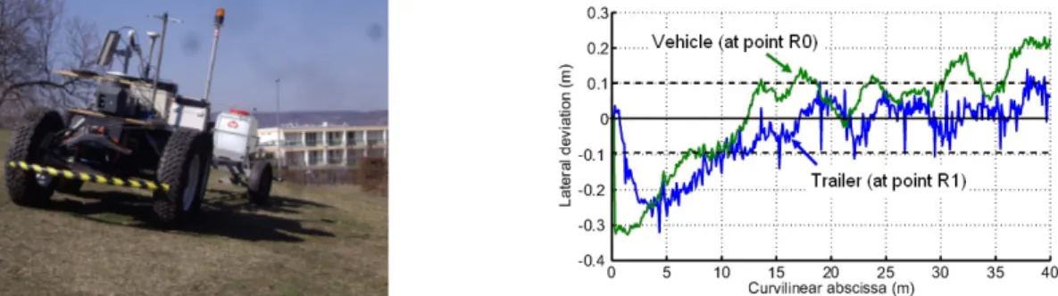
• Curved path following: as a first step, to point out that the trailer does not follow the vehicle's track on such a reference path, path following is performed at 1.4m/s with respect to the vehicle lateral and angular deviations (y0, 110), i.e. the trailer is ignored in that case. The

results are presented in Fig. 11.The lateral deviations y0 and y1 of the vehicle and the trailer

with respect to Γ are plotted according to the curvilinear abscissa. It can be seen that the vehicle follows satisfactorily Γ, whereas the trailer is shifted inside the two successive circles. The vehicle starts at about 18cm from Γ, then, it reaches Γ and maintains an overall lateral error within ±10cm (except at the beginning of the first circle, at curvilinear abscissa 17m, due to a fast curvature variation and actuator delays). In contrast, the trailer is shifted for roughly 50cm during the first circle and for more than 30cm during the second one.

FIGURE 11: Curved path following with respect to the vehicle

In the second test, the proposed control law (8) has been used in order to control the position of the trailer with respect to Γ. The results are depicted in Fig.12. It can be seen that the vehicle has moved outside the two successive circles (for roughly 40cm) enabling an accurate path tracking for the trailer. The trailer starts at about 30cm from Γ, then, it reaches

Γ and maintains a satisfactory overall lateral error within ±10cm.

FIGURE 12: Curved path following with respect to the trailer

• Straight line following in a sloping field: a heavy water drum has been added at the extremity of the trailer in order to obtain significant sliding phenomena in slope. A straight line is then recorded during a manual run on an irregular and side sloped ground varying from 0 to 25%. Path following is then achieved with control law (8). It can be seen in Fig. 13 that the trailer follows satisfactorily the reference path Γ despite the variation in the slope, with an overall error within ±10cm. It can be noticed that the vehicle moves away from the reference trajectory Γ for about 10cm in order to keep the trailer correctly on Γ.

• Backward path following and reverse turn maneuver: a reference path Γ is first recorded with the GPS receiver during a manual run. Then, path following is achieved backward at 0.5m/s with the proposed control law (8). It can be seen in Fig. 14 that the trailer starts with a lateral deviation of 1m from Γ. Then, it reaches the planned path and maintains an overall lateral error of about ±20cm.

Figure 14: Backward path following

The proposed control law (8) has finally been used to control the trailer backward between the two stop points S1 and S2 in a reverse turn maneuver, see Fig. 15.

FIGURE 15: Reverse turn maneuver

5. Conclusion

This paper addresses the problem of accurate path following of a vehicle-trailer system in presence of sliding, with application to automatic guidance of a towed agricultural implement. The objective is to control the position of the trailer's center with respect to a planned trajectory. An extended kinematic model accounting for sliding effects via three side slip angles has first been considered and an observer is used to obtain relevant estimations of the side slip angles. Next, a control law has been designed according to three steps. Promising results, based on full scale experiments, have been presented: the proposed algorithms succeed in stabilizing the trailer with a satisfactory overall lateral error within ±10cm during forward path following, and within ±20cm during backward motions.

References

Kormann G., Thacher R (2008). Development of a passive implement guidance system. International conference on agricultural engineering, Hersonissos-Crete, Greece.

Lenain R., Thuilot B., Cariou C., Martinet P. (2006). Sideslip angles observers for vehicle guidance in sliding conditions: application to agricultural path tracking task. IEEE conf. on Robotics and Automation, Florida, USA, pp. 3183-3158.

Wang D., Low C. B. (2006). Modeling skidding and slipping in wheeled mobile robots: control design perspective. IEEE int. conf. on Intelligent Robots and Systems, Beijing, China.