HAL Id: hal-00159580
https://hal.archives-ouvertes.fr/hal-00159580
Submitted on 3 Jul 2007HAL is a multi-disciplinary open access archive for the deposit and dissemination of sci-entific research documents, whether they are pub-lished or not. The documents may come from teaching and research institutions in France or abroad, or from public or private research centers.
L’archive ouverte pluridisciplinaire HAL, est destinée au dépôt et à la diffusion de documents scientifiques de niveau recherche, publiés ou non, émanant des établissements d’enseignement et de recherche français ou étrangers, des laboratoires publics ou privés.
Computing commons interval of K permutations, with
applications to modular decomposition of graphs
Anne Bergeron, Cedric Chauve, Fabien de Montgolfier, Mathieu Raffinot
To cite this version:
Anne Bergeron, Cedric Chauve, Fabien de Montgolfier, Mathieu Raffinot. Computing commons inter-val of K permutations, with applications to modular decomposition of graphs. ESA’05, 13th Annual European Symposium on Algorithms, 2005, Majorque, Spain. pp.779-790. �hal-00159580�
Computing common intervals of K permutations, with
applications to modular decomposition of graphs
Anne Bergeron∗ Cedric Chauve∗ Fabien de Montgolfier† Mathieu Raffinot‡
Abstract
We introduce a new way to compute common intervals of K permutations based on a very simple and general notion of generators of common intervals. This formalism leads to simple and efficient algorithms to compute the set of all common intervals of K permutations, that can contain a quadratic number of intervals, as well as a linear space basis of this set of common intervals. Finally, we show how our results on permutations can be used for computing the modular decomposition of graphs in linear time.
1
Introduction
The notion of common interval was introduced in [16] in order to model the fact that a group of genes can be rearranged in a genome but still remain connected. In [16], Uno and Yagiura proposed a first algorithm that computes the set of common intervals of a permutation P with the identity permutation in time O(n + N ), where n is the length of P , and N is the number of common intervals. However, N can be of size O(n2), thus the algorithm of Uno and Yagiura has a O(n2) time complexity. Heber and Stoye [10] defined a subset of the common intervals of K permutations, called irreducible common intervals, that contains O(n) common intervals and forms a basis of the set of all common intervals: every common interval is a chain overlapping irreducible common intervals. They proposed an O(Kn) time algorithm to compute the set of irreducible common intervals of K permutations, based on Uno and Yagiura’s algorithm.
One of the drawbacks of these algorithms is that properties of Uno and Yagiura’s algo-rithm are difficult to understand: even the authors describe their O(n + N ) algoalgo-rithm as ”quite complicated”. In practice, simpler O(n2) algorithms run faster on randomly generated permutations [16]. On the other hand, Heber and Stoye’s algorithms rely on a complex data structure that mimics what is known, in the theory of modular decomposition of graphs, as the P Q-trees of strong intervals. An incentive to revisit this problem is the central role that these P Q-trees seem to play in the field of comparative genomics. Strong intervals can be used to identify significant groups of genes that are conserved between genomes [11], or as guides to reconstruct plausible evolution scenarios [1, 7].
∗LaCIM, Universit´e du Qu´ebec `a Montr´eal, Canada. E-mail: [anne,chauve]@lacim.uqam.ca
†LIAFA, Universit´e Denis Diderot - Case 7014, 2 place Jussieu, F-75251 Paris Cedex 05, France. E-mail: [email protected]
‡CNRS - Laboratoire G´enome et Informatique, Tour Evry 2, 523, Place des Terrasses de l’Agora, 91034 Evry, France. E-mail: [email protected]
In order to design alternative efficient algorithms to compute common intervals, we pro-pose a theoretical framework for common intervals based on generating families of intervals. These families can be computed by straightforward O(n) algorithms that use only tables and stacks as data structures, and that upgrade trivially to the case of K permutations. Using these families, we compute common intervals with simple O(n + N ) and O(n) algorithms whose properties can be readily verified. We then link this work to previous studies on common interval, and we propose a new canonical representation of the family of common intervals that is simpler than the P Q-tree in many applications, and we exhibit the tight links between these two representations.
Finally, we extend our approach to the classical graph problem of modular decomposition that aims to efficiently compute a compact representation of the modules of a graph. The first linear time algorithms that appeared in 1994 [12, 5] are rather complex and many studies have been undertaken to design decomposition algorithms that are efficient in practice, even if they do not run in linear time but in quasi-linear time [6, 13]. The current simplest algorithm works in two steps. It first computes a factorizing permutation and then builds a tree representation on it. The first step has been simplified in [15, 8]. In this paper, we simplify the second step. The article is structured as follows. In Section 2, we describe the notion of generator of common interval and how to compute a generator in O(Kn) time. The third section explains how to generate the set of common intervals in O(n + N ) from the generator. Section 4 describes a new compact basis of common intervals, called canonical generators, and describes the links between this new basis and the classical basis of strong intervals and P Q-trees. Section 5 contains a simple linear-time algorithm to construct the strong intervals based, given a canonical generator. Finally, in Section 6, we extend our results to the modular decomposition of graphs.
2
Common intervals and generators
A permutation P on n elements is a complete linear order on the set of integers{1, 2, . . . , n}. We denote Idn the identity permutation (1, 2, . . . , n). An interval of a permutation P =
(p1, p2, . . . , pn) is a set of consecutive elements of permutation P . An interval of a permutation
will be denoted by either giving its left and right bounds, such as [i, j], or by giving the list of its elements, such as (pi, pi+1, . . . , pj). An interval [i, j] = (i, i + 1, . . . , j) of the identity
permutation will be simply denoted by (i..j).
Definition 1 LetP = {P1, P2, . . . , PK} be a set of K permutations on n elements. A common
interval ofP is a set of integers that is an interval in each permutation of P.
The set{1, 2, . . . , n} and all singletons are always common intervals of any non empty set of permutations, they are called trivial intervals. In the sequel, we will assume that the setP contains the identity permutation Idn. A common interval of P can thus be denoted as an
interval (i..j) of the identity permutation.
Definition 2 Let P = {Idn, P2, . . . , PK} be a set of K permutations on n elements. A
generator for the common intervals ofP is a pair (R, L) of vectors of size n such that: 1. R[i]≥ i and L[j] ≤ j for all i, j ∈ {1, 2, . . . , n},
The following proposition shows that constructing a generator for a union of sets of per-mutations is simple, once generators are known for each set. If X and Y are two vectors, we denote by min(X, Y ) the vector min(X[1], Y [1]), . . . , min(X[n], Y [n]).
Proposition 1 Let (R1, L1) and (R2, L2) be generators for the common intervals of two
sets P1 and P2 of permutations, both containing the identity permutation, then the pair
(min(R1, R2), max(L1, L2)) is a generator for the common intervals of P1∪ P2.
Proof. First note that (i..j) = (i..R[i])∩ (L[j]..j) if and only if L[j] ≤ i ≤ j ≤ R[i]. Interval (i..j) is a common interval of P1∪ P2 if and only if it is a common interval of both P1 and
P2, which is equivalent to L1[j] ≤ i ≤ j ≤ R1[i] and L2[j] ≤ i ≤ j ≤ R2[i], and then to
max(L1[j], L2[j])≤ i ≤ j ≤ min(R1[i], R2[i]). 2
Proposition 1 implies that, given an O(n) algorithm for computing generators for the com-mon intervals of two permutations, we can easily deduce an O(Kn) algorithm for computing a generator for the common intervals of K permutations. Generators are far from unique, but some are easier to compute than others. Identifying good generators is a crucial step in the design of efficient algorithms to compute common intervals. The remaining of this section focuses on particular classes of generators that turn out to have interesting properties with respect to computations.
Definition 3 Let P = (p1, . . . , pn) be a permutation on n elements. For each element pi,
define:
IM ax[pi] to be the largest interval of P that contains pi, and no element smaller than pi,
IM in[pi] to be the largest interval of P that contains pi, and no element greater than pi,
Sup[pi] to be the largest integer such that (pi..Sup[pi])⊆ IMax[pi],
Inf [pi] to be the smallest integer such that (Inf [pi]..pi)⊆ IMin[pi].
Remark that (pi..Sup[pi]) and (Inf [pi]..pi) are intervals of the identity permutation, but not
necessarily intervals of permutation P . For example, if P = (1 4 7 5 9 6 2 3 8), we have: IM ax[5] = (7 5 9 6) and Sup[5] = 7, and IM in[8] = (6 2 3 8) and Inf [8] = 8.
Proposition 2 The pair of vectors (Sup, Inf ) is a generator for the common intervals of P and Idn.
Proof. Suppose that (i..j) is a common interval of P and Idn, then Sup[i]≥ j and Inf[j] ≤ i
since all element in the set (i..j) are consecutive in permutation P , thus (i..j) = (i..Sup[i])∩ (Inf [j]..j). On the other hand, suppose that Sup[i] ≥ j and Inf[j] ≤ i, then IMax[i] contains j and IM in[j] contains i. Since both IM ax[i] and IM in[j] are intervals of P , their intersection is an interval and is equal to (i..j). 2
Proposition 3 Let P be a permutation on n elements. If the bounds of intervals IM ax[k] and IM in[k] are known for all k, then Algorithm 1 computes (Sup, Inf ) in O(n) time.
Proof. We first show that the Algorithm 1 is correct. Suppose that, at the beginning of the k-th iteration of the second For loop, Inf [k0] = m[k0] for all k0 < k, and m[k] ∈ IMin[k]. This is clearly the case at the beginning of iteration k = 2, since Inf [1] = 1. By definition, Inf [k]≤ k, thus before entering the While loop, we have Inf[k] ≤ m[k]. If the test m[k]−1 ∈
Algorithm 1: Computing the generator (Sup, Inf ). Inf [1]← 1, Sup[n] ← n. For k from 1 to n, m[k]← k, M[k] ← k. For k from 2 to n While m[k]− 1 is in IMin[k], m[k] ← m[m[k] − 1] Inf [k]← m[k] For k from n− 1 to 1 While M [k] + 1 is in IM ax[k], M [k]← M[M[k] + 1] Sup[k]← M[k]
IM in[k] of the While loop is true, then Inf [k]≤ m[k] − 1, implying Inf[k] ≤ Inf[m[k] − 1]. Since Inf [m[k]− 1] = m[m[k] − 1] by hypothesis, the instruction in the While loop preserves the invariant Inf [k]≤ m[k]. When the test of the While loop becomes false, then Inf[k] is greater than m[k]− 1, thus Inf[k] = m[k]. The correctness of Sup has a similar proof.
Suppose that IM in[k] = [i, j], then the tests in the While loops can be done in constant time using the inverse of permutation P . The total time complexity follows from the fact that the instruction within the While loop is executed exactly n− 1 times. Indeed, consider, at any point of the execution of the algorithm, the collection of intervals (m[k]..k) of the identity permutation that are not contained in any other interval of this type. After the initialization loop, we have n such intervals, and at the completion of the algorithm, there is only one, namely (1..n), since Inf [n] = 1. The instruction in the While loop merges two consecutive intervals into one and there can be at most n− 1 of these merges. 2
The computation of the bounds of intervals IM ax[k] and IM in[k], as well as the compu-tation of the inverse of permucompu-tation P , are quite straightforward. As an example, Algorithm 2 shows how to compute the left bound of IM ax[pi].
Algorithm 2: Computing the left bound LM ax[pi] of IM ax[pi] for all pi
S is a stack of positions; s denotes the top of S. Push 0 on S
p0 ← 0
For i from 1 to n
While pi< ps Pop the top of S
LM ax[pi]← s + 1
Push i on S
Proposition 4 Let P = (p1, . . . , pn) be a permutation on n elements, Algorithm 2 computes
the left bound of all intervals IM ax[pi] in O(n) time.
Proof. The time complexity of Algorithm 2 is immediate since each position is stacked once. The correctness of LM ax relies on the fact that, at the beginning of the i-th iteration, the position j of the nearest left element such that pj < pi must be in the stack. If it was not the
case, then an element smaller than pj was found between the positions j and i, contradicting
the definition of position j. 2
To summarize the results of this section, we have:
Theorem 1 Let P = {Idn, P2, . . . , PK} be a set of K permutations on n elements. It is
3
Common intervals of K permutations in O(Kn + N ) time
We now turn to the problem of generating all common intervals of K permutations in O(N ) time, where N is the number of such common intervals, given a generator satisfying the following property.
Definition 4 Two sets A and B commute if either A⊆ B, or B ⊆ A, or A and B are disjoint, and otherwise they overlap. A collectionC of sets is commuting if, for any pair A and B in C, A and B commute.
A generator (R, L) for the common intervals of P = {Idn, P2, . . . , PK} is commuting if
both the collections{(i..R[i])}i∈(1..n) and{(L[i]..i)}i∈(1..n) are commuting.
If (R, L) is a commuting generator, define Support[i], for i > 1, to be the greatest integer j < i such that R[i]≤ R[j].
It turns out that all generators defined in Section 2 are commuting: generators com-puted by Proposition 1 are commuting if they are constructed with commuting genera-tors R1, L1, R2, L2. This is a consequence of the fact that if a < b and a0 < b0 then
min(a, a0) < min(b, b0) and max(b, b0) > max(a, a0). For the basic generators, we have:
Proposition 5 The generator (Sup, Inf ) for the common intervals of permutations P and Idn is commuting.
Proof. Suppose that (k..Sup[k]) contains k0, we will show that it must also contain Sup[k0]. If k0 is in (k..Sup[k]), then k0 is in IM ax[k], and k0 > k, therefore, IM ax[k0] ⊆ IMax[k], and the interval (k0..Sup[k0]) is included in IM ax[k], thus in (k..Sup[k0]) also. Since Sup[k] is maximal, we must have Sup[k]≥ Sup[k0]. A similar argument holds for Inf . 2
Algorithm 3: Computing Support[i] for a commuting generator (R, L) S is an empty stack; s denotes the top of S
Push 1 on S For i from 2 to n
While R[s] < i Pop the top of S Support[i]← s
Push i on S
Proposition 6 Given a commuting generator (R, L), Algorithm 3 computes the values Support[i], for all i > 1, in linear time.
Proof. The time complexity of Algorithm 3 is immediate. At iteration i the stack contains the left bounds of all intervals of (j..R[j]) such that R[j]≥ i and j < i, sorted in decreasing size order. It is then easy to see when equality holds. Note that Support[1] is undefined and should not be used by subsequent algorithms. 2
Proposition 7 Given a commuting generator (R, L), Algorithm 4 outputs all common inter-vals of a setP of K permutations on n elements, in O(n + N) time, where N is the number of common intervals of the set P.
Proof. The time complexity of Algorithm 4 is immediate. Suppose that interval (i..j) is identified by the algorithm. At the start of the j-th iteration, i = j, thus j≤ R[i]. If the test of the While loop is true, then i≥ L[j], and (i..j) is a common interval. If i0 = Support[i], then R[i0]≥ R[i], thus j ≤ R[i0] at the end of the While loop.
On the other hand, if (i..j) is a common interval of P, with i < j, then Support[j] ≥ i, since R[i] ≥ R[j]. Let i0 be the smallest integer such that i < i0 and (i0..j) is identified by Algorithm 4 as a common interval. Such an interval exists, since (j..j) is a common interval. We will show that Support[i0] = i. Indeed, Support[i0] must be greater than or equal to i. If it is greater, then (Support[i0]..j) is a common interval, contradicting the definition of i0. 2
Algorithm 4: Generating the common intervals of a setP given a generator (R, L) For j from n to 1
i← j
While i≥ L[j]
Output (i..j) (* Interval (i..j) is a common interval of the setP *) i← Support[i]
4
Canonical representations of closed families
The common intervals of a set of permutations is an example of a more general families of intervals, the closed families. In this section, we develop a new canonical representation for such families, based on the generators of the previous section.
A closed familyF of intervals of the identity permutation on n elements is a family that contains all singletons, the interval (1..n) and that has the following property: if (i..k) and (j..l) are in F, and i ≤ j ≤ k ≤ l, then (i..j), (j..k), (k..l) and (i..l) belong to F.
Closed families can have a quadratic number of elements, but can be compactly represented by P Q-trees:
Definition 5 A P Q-tree is a tree whose leaves are labeled from 1 to n, whose internal nodes are labeled P -nodes or Q-nodes, such that a P -node has at least two children, such that a Q-node has at least three children, and such that the children of a Q-node are totally ordered.
A classical result [2] establishes a bijection between the P Q-trees with n leaves and closed families of Idn, thus allowing a representation of size O(n) for any closed family. It is easy to
extend Definition 2 to the more general case of closed families. Among all possible generators, the following ones will also provide a representation of size O(n) for any closed family:
Definition 6 A generator (R, L) for a closed family F is canonical if, for all i ∈ (1..n), intervals (i..R[i]) and (L[i]..i) belong to F.
Proposition 8 LetF be a closed family. The canonical generator of F always exists, and it is unique and commuting.
Proof. LetF be a closed family. For 1 ≤ i ≤ n, define R[i] be the largest integer such that (i..R[i])∈ F, and L[i] be the smallest integer such that (L[i]..i) ∈ F.
If an interval (i..j) ∈ F, then (i..j) ⊆ (i..R[i]), and (i..j) ⊆ (L[j]..j), thus (R, L) is a generator. It is canonical since we picked elements of F. Suppose that there exists a second
canonical generator (R0, L0), with R6= R0, then there exists 1≤ i ≤ n such that R0[i] < R[i].
Since (i..R[i]) is inF, it should be generated by (R0, L0) but (i..R0[i])∩(L0[R[i]], R[i]) does not contain R[i]. A similar argument holds if L6= L0. Finally, suppose that two intervals (i..R[i]) and (j..R[j]) overlap with i < j < R[i] < R[j]. Then (i..R[j]) is in F which contradicts the maximality of (i..R[i]). 2
Algorithm 5: Computing the canonical generator (R, L) given any generator (R0, L0) The vector Support is obtained from R0 using Algorithm 3
R[1]← n
For k from 2 to n R[k]← k For k from n to 2
If (Support[k]..R[k])∈ F
R[Support[k]]← max(R[k], R[Support[k]])
(* Computation of L is similar, by defining the vector Support with respect to L0 *) Theorem 2 Algorithm 5 computes the canonical generator (R, L) of a closed family F, in O(n) time, given a commuting generator (R0, L0).
Proof. The time complexity of Algorithm 5 follows from the fact that testing if an interval belongs toF can be computed in O(1) time with the generator (R0, L0). Its correctness relies on the following observation: if R[k]6= k, then there exists an integer k0> k such that
Support[k0] = k, and R[k0] = R[k] (1)
where Support[k0] is defined (Definition 4) as the greatest integer smaller than k0 such that R0[Support[k0]] ≥ R0[k0]. Statement (1) implies that, since the values of R[k] are computed in decreasing order, the value of R[k] will be known at the start of iteration k.
In order to prove statement (1), let k0 be the smallest integer such that R[k0] = R[k]. The hypothesis R[k]6= k, and the fact that (R, L) is a commuting generator, imply that k0 > k. We must show that Support[k0] = k. Since (R0, L0) is a commuting generator, and (R, L) is the canonical generator, we must have R0[k] ≥ R0[k0]. Thus, Support[k0] ≥ k, implying
that R[Support[k0]] ≤ R[k]. Since R[k] = R[k0], this would imply R[Support[k0]] = R[k], contradicting the definition of k0. 2
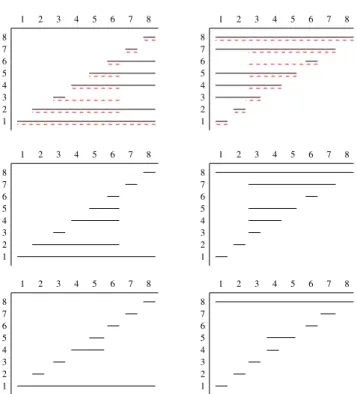
Example 1 As an example, let P = {Id8, P2} and Q = {Id8, P3} with
Id8 = (1, 2, 3, 4, 5, 6, 7, 8) P2 = (1, 3, 2, 4, 5, 7, 6, 8) P3 = (2, 8, 3, 4, 5, 6, 1, 7)
Figure 1 shows the generators (Sup, Inf ) for the common intervals ofP and of Q, a generator for the common intervals of P ∪ Q built on the two first ones, and the canonical generator for the common intervals of P ∪ Q.
Compared to P Q-trees, this canonical representation of a closed familyF is much simpler since it basically relies on two arrays. Moreover, some operations, for instance testing if an interval (i..j) belongs to the family F, are also simpler on it. However, the P Q-tree has the advantage of being a recursive structure. Thus, in order to be complete, we show below how to transform one representation into the other using the key notion of strong intervals.
8 7 6 5 4 3 2 1 8 7 6 5 4 3 2 1 8 7 6 5 4 3 2 1 8 7 6 5 4 3 2 1 8 7 6 5 4 3 2 1 8 7 6 5 4 3 2 1 1 2 3 4 5 6 7 8 1 2 3 4 5 6 7 8 1 2 3 4 5 6 7 8 1 2 3 4 5 6 7 8 1 2 3 4 5 6 7 8 1 2 3 4 5 6 7 8
Figure 1: The top row shows the generators (Sup, Inf ) of the common intervals of the set P in solid lines, and of set Q in dashed lines. The middle row, a generator for the common intervals ofP ∪ Q is constructed using Proposition 1. Finally, the bottom row is the canonical generator constructed by Algorithm 5
5
From canonical generators to strong intervals and P Q-trees
A strong interval of F is an interval that commutes with each interval of F. In [15], it is shown that the P Q-tree associated to F is the inclusion tree of the strong intervals. In this section, we show how to compute the strong intervals, given a canonical generator.
Let (R, L) be the canonical generator. Consider the 4n bounds of intervals of the families (i..R[i]) and (L[j]..j) for i, j ∈ (1..n). Let (a1, . . . , a4n) be the list of these 4n bounds sorted
in increasing order and, if equality, with the left bounds sorted before the right bounds. For the example Figure 1 the list is
(1, 1, 1, 1, 2, 2, 2, 2, 3, 3, 3, 3, 4, 4, 4, 4, 5, 5, 5, 5, 6, 6, 6, 6, 7, 7, 7, 7, 8, 8, 8, 8)
where i denotes a right bound. This list can be constructed easily by scanning the two vectors R and L, and by noting that each i∈ (1..n) is a left bound at least once, and a right bound at least once.
Proposition 9 Given the ordered list (a1, . . . , a4n) of the 4n bounds of a canonical generator
(R, L), Algorithm 6 outputs the strong intervals of a closed family in O(n) time.
Proof. An interval of the form (i..R[i]) non-trivially overlap intervals of the form (L[j]..j) only if i ≤ j < R[i], otherwise R[i] would not be maximal. If (i..R[i]) is identified by the algorithm, then (i..R[i]) must commute with all intervals of the form (L[j]..j), therefore with
Algorithm 6: Computation of the strong intervals S is a stack of bounds, s denotes the top of S
For i from 1 to 4n If ai is a left bound
Push ai on S
Else
Output (s..ai) (* Interval (s..ai) is strong *)
Pop the top of S
all members ofF, implying (i..R[i]) is a strong interval. A similar argument shows that any interval of the form (L[j]..j) that is identified by the algorithm must be strong.
If an interval (i..j) is identified by Algorithm 6, but is neither of the form (i..R[i]) or (L[j]..j), then it must be the intersection of the two, therefore (i..j) ∈ F since (R, L) is a generator. If (i..j) is not a strong interval, then there exists k such that either i < k≤ j and R[k] > j, or i≤ k < j and L[k] < i. In the first case, all the intervals of the form (i..R[i]) that end at j have a left bound greater of equal to k, implying that j is paired only to values greater or equal to k by the algorithm, thus (i..j) is not identified. A similar argument holds for the other case.
Define δ(k, l) to be the difference between the number of left bounds and the number of right bounds in the sublist of (a1, . . . , a4n) that begins at position k a and ends at position
l. Let (i..j) be a strong interval, p(i) the last position of i in the list of bounds, and p(j) the first position of j in the list of bounds. Let x be the number of integers j0 such that L[j0] = i and j0 < j, and y be the number of integers i0 such that R[i0] = j and i0 > i. We have δ(p(i), p(j)) = y− x. But, since R[i] ≥ j and L[j] ≤ i, there are at least x + 1 left bounds i and at least y + 1 right bounds j in the list. Thus Algorithm 6 outputs the interval (i..j). 2
6
Modular decomposition
Let G = (V, E) be a directed, finite, loopless graph, with|V | = n and |E| = m. Undirected graphs may be seen as symmetrical directed graphs in this context. A module is a subset M of V that behaves like a single vertex: for x /∈ M either there are |M| arcs that join x to all vertices of M , or no arc joins x to M , and conversely either there are |M| arcs that join all vertices of M to x, or no arc joins M to x. A strong module does not overlap any other module. There may be up to 2n modules in a graph (in the complete graph for instance)
but there are at most O(n) strong modules, and the modular decomposition tree based on the strong modules inclusion tree is sufficient to represent all modules [14].
Modular decomposition is the first step in many graph algorithms like graph recognition (eg. cographs, interval graphs, permutation graphs and other classes of perfect graphs, see [3] for a survey) and transitive orientation computation [12]. (See [14] for a survey.)
Many linear-time decomposition algorithms have been discovered ([12, 5, 6]) but remain rather complex. This is why, in the late 90’s, some research attempted to design practical modular decomposition algorithms, sometimes at the price of a less efficient – is obtained by noticing – theoretical complexity. In [13], an O(n + m log n) algorithm was proposed while [6] gives an O(n+mα(n, m)) complexity bound (where α(n, m) is the inverse Ackermann function). The current simple algorithms work in two steps. They first compute a factorizing
permutation, and then compute the modular decomposition tree on it. We simplify below the second step.
A factorizing permutation of a graph [4] is a permutation of the vertices of the graph in which every strong module of the graph is a factor. As the strong modules are a commuting family, every graph admits a factorizing permutation. As noticed by Hsu and Ma [9], the LexBFS graph traversal produces a factorizing permutation of a chordal graph. A factorizing permutation of a graph can be computed in linear time [8]. In the following we assume, without loss of generality, that the vertex-set V is the set {1, ..n} and that the identity permutation is a factorizing permutation of the graph.
Given an interval (u..v) of the factorizing permutation, a vertex x /∈ (u..v) is a splitter of the interval if there are between 1 and v− u arcs going from x to (u..v) or if there are between 1 and v− u arcs going from (u..v) to x. A right-module is an interval (u..v) with no splitters greater than v. A left-module is an interval (u..v) with no splitters smaller than u. An interval-module is an interval (u..v) with no splitters. Clearly interval-modules are modules. However, all modules are not interval-modules, but according to the definition of a factorizing permutation, the strong modules of the graph are interval-modules. A classical result is that modules behave like intervals: the union, intersection or difference of two overlapping module is a module. Thus:
Proposition 10 [14] The interval-modules of a factorizing permutation are a closed family. The strong intervals of this family are exactly the strong modules of the graph.
Definition 7 For a vertex v let R[v] be the greatest integer such that (v..R[v]) is a left-module and L[v] the smallest integer such that (L[v]..v) is a right-module.
It can be easily proved that for every w∈ (L[v]..v), (w..v) is a right-module, and for every w < L[v], (w..v) is not a module. For this reason (L[v]..v) is called the maximal right-module ending at v. We can also define the maximal left-right-module beginning at v. According to this property and to the deifnition of interval-modules, we have:
Proposition 11 The pair (R, L) is a commuting generator of the interval-modules family.
Proof. Clearly (u..v) is an interval-module if and only if R[u]≥ v and L[v] ≤ u, and so (R, L) is a generator. R is commuting because if (u..R[u]) overlaps (v..R[v]), and if, without loss of generality, u < v, (u..R[v]) is a left-module starting at u greater than the maximal left-module (u..R[u]), which is a contradiction. A similar proof shows that L also is commuting. 2
Hence, we would like to know how to compute the maximal right-strong and left-strong modules. The following algorithm is a simplified version of an algorithm due to Capelle and Habib [4] for computing the maximal right-modules. The algorithm to compute the maximal left-modules can easily be derived from it.
Let us consider the maximal right-module (L[v]..v) ending at v. If L[v] > 1, then there exists an x > v that splits (L[v]− 1..v), otherwise this right-module would not be maximal, and x therefore splits (L[v]− 1..L[v]), but does not split (y − 1, y) for all L[v] < y ≤ v.
Based on this observation, Capelle and Habib algorithm proceeds in two steps. First, for every vertex v the rightmost splitter s[v] is computed. It is the greatest vertex, if any, that splits the pair (v − 1..v). Then a loop for v from n to 2 computes all the maximal right-modules (L[x]..x) such that v = L[x].
Computing s[v] can be done by a simultaneous scan of the adjacency lists of v and v− 1: the greatest element occurring in only one adjacency list is kept. It takes a time linear in the adjacency lists size. The computation of s[v] for all v can therefore be performed in O(n + m), that is linear in the size of the graph. The second step is Algorithm 7. It clearly runs in O(n) time. Its correctness relies on the following invariant:
Invariant At step v, for all vertices x in the stack, (v..x) is a right-module, and for all x > v not in the stack, L[v] > v.
Proof. The invariant is initially true. Every step maintains it: if s[v] does not exist then for all x in the stack (v− 1..x) is a right-module, and (v − 1..v) also is a right-module. And if s[v] exists, (v) is the maximal right-module ending at v. For all x < s[v] (v− 1..x) is not a right-module and (v..x) is therefore the maximal right-module ending at x. For all x≥ s[v] (v− 1..x) is still a right-module, because s[v] is the greatest of the splitters of (v − 1, v). 2
Algorithm 7: Computing all maximal right-modules S is a stack of vertices; t denotes the top of S.
for v from n to 2 if s[v] exists
L[v]← v While t < s[v]
L[t]← v
Pop the top of S else
Push v on S
We thus have:
Theorem 3 Given a graph G, and a factorizing permutation of G, it is possible to compute the modular decomposition tree of G in time O(n + m).
7
Conclusion
In the present work, we formalized two concepts about common intervals, namely generators and canonical representation, that prove to have important algorithmic implications. Indeed, the combinatorial properties of these objects, and in particuliar the different links between them, are central in the design and the analysis of the simple optimal algorithms for com-puting common intervals of permutations we presented. It is important to highlight that our algorithms are ”real optimal algorithm” as they are based on very elementary manipulations of stacks and arrays. This is, we believe, a significant improvment over the existing algorithms that are based on intricate data structures, in terms of ease of implementation, time efficiency and understanding of the underlying concepts [16, 10].
Moreover, we showed how, transposed in the more general context of modular decomposi-tion of graphs, our results have a similar impact and lead to a significant simplificadecomposi-tion of some existing algorithms. Indeed, modular decomposition algorihms are quite complex algorithms, but using the simple factorizing permutation algorithm of [8] and then the right-modules iden-tification algorithm we presented, a generator of the interval-modules can easily be computed in linear time; tools from Section 5 can then be used to compute the strong interval-modules,
that also are the strong modules, and the P Q-tree, called modular decomposition tree in this context.
References
[1] S. B´erard, A. Bergeron, and C. Chauve. Conserved structures in evolution scenarios. In Compar-ative Genomics, RECOMB 2004 International Workshop, vol. 3388 of Lecture Notes in Comput. Sci., p. 1–15. Springer-Verlag, 2005.
[2] S. Booth and G. Lueker. Testing for the consecutive ones property, interval graphs, and graph planarity using PQ-trees algorithms. J. Comput. Syst. Sci., 13:335–379. 1976.
[3] A. Brandst¨adt, V.B. Le, and J. Spinrad. Graph Classes: a Survey. SIAM Monographs on Discrete Mathematics and Applications. SIAM, 1999.
[4] C. Capelle and M. Habib. Graph decompositions and factorizing permutations. in Fifth Israel Symposium on Theory of Computing and Systems, ISTCS 1997, p. 132–143. IEEE Computer Society, 1997.
[5] A. Cournier and M. Habib. A new linear algorithm for modular decomposition. In Trees in algebra and programming – CAAP’94, 19th International Colloquium, vol. 787 of Lecture Notes in Comput. Sci., p. 68–84. Springer-Verlag, 1994.
[6] E. Dahlhaus, J. Gustedt, and R. M. McConnell. Efficient and practical algorithms for sequential modular decomposition. J. Algorithms, 41(2):360–387. 2001.
[7] M. Figeac and J.-S. Varr´e. Sorting by reversals with common intervals. In Algorithms in Bioin-formatics, 4th International Workshop, WABI 2004, vol. 3240 of Lecture Notes in Comput. Sci., p. 26–37. Springer-Verlag, 2004.
[8] M. Habib, F. de Montgolfier and C. Paul. A Simple Linear-Time Modular Decomposition Algo-rithm for Graphs, Using Order Extension In AlgoAlgo-rithm Theory – SWAT 2004, 9th Scandinavian Workshop on Algorithm Theory, vol. 3111 of Lecture Notes in Comput. Sci., p. 187–198. Springer-Verlag, 2004.
[9] W.-L. Hsu and T.-H. Ma Substitution decomposition on chordal graphs and applications In ISA’91 Algorithms, International Symposium on Algorithms, vol. 557 of Lecture Notes in Comput. Sci., p. 52–60. Springer-Verlag, 1991.
[10] S. Heber and J. Stoye. Finding all common intervals of k permutations. In Combinatorial Pattern Matching, 12th Annual Symposium, CPM 2001, vol. 2089 of Lecture Notes in Comput. Sci., p. 207–218. Springer-Verlag, 2001.
[11] G.M. Landau, L. Parida and O. Weimann. Gene Proximity Analysis Across Whole Genomes via PQ Trees. Submitted, 2004.
[12] R. M. McConnell and J. Spinrad. Linear-time modular decomposition and efficient transitive orientation of comparability graphs. In Fifth Annual ACM-SIAM Symposium on Discrete Algo-rithms, p. 536–545. ACM/SIAM, 1994.
[13] R. M. McConnell and J. Spinrad. Ordered vertex partitioning. Discrete Mathematics & Theoret-ical Computer Science, 4:45–60. 2000.
[14] R. H. M¨ohring and F. J. Radermacher. Substitution decomposition for discrete structures and connections with combinatorial optimization. Annals of Discrete Mathematics, 19:257–356. 1984. [15] F. de Montgolfier. D´ecomposition modulaire des graphes. Th´eorie, extensions et algorithmes.
Ph.D. thesis, Montpellier II University (France). 2003.
[16] T. Uno and M. Yagiura. Fast algorithms to enumerate all common intervals of two permutations. Algorithmica, 26(2):290–309 2000.