Database partitioning strategies for social network data

(1)

Database Partitioning Strategies for Social

Network Data

by

Oscar Ricardo Moll Thomae

B.S. EECS, Massachusetts Institute of Technology (2011)

B.S. Mathematics, Massachusetts Institute of Technology (2011)

Submitted to the Department of Electrical Engineering and Computer

Science

in partial fulfillment of the requirements for the degree of

Masters of Engingeering in Electrical Engineering and Computer

Science

at the

ARCHIVES>

MASSACHUSETTS INSTITUTE OF TECHNOLOGY

June 2012

@

Massachusetts Institute of Technology 2012. All rights reserved.

IA

Author ... ... ...

Department of Electrical Engineering ah1lComputer Science

May 25, 2012

Certified by.

r--.

Certified

by...

(7>-V

Stu Hood

Engineer at Twitter

Company Supervis

Samuel R. Madden

Associate Professor

MIT Thesis

SInervisor

Accepted by ...

Dennis M. Freeman

Chairman, Masters of Engineering Thesis Committee

(2)

Database Partitioning Strategies for Social Network Data by

Oscar Ricardo Moll Thomae

Submitted to the Department of Electrical Engineering and Computer Science on May 25, 2012, in partial fulfillment of the

requirements for the degree of

Masters of Engingeering in Electrical Engineering and Computer Science

Abstract

In this thesis, I designed, prototyped and benchmarked two different data partitioning strategies for social network type workloads. The first strategy takes advantage of the heavy-tailed degree distributions of social networks to optimize the latency of vertex neighborhood queries. The second strategy takes advantage of the high temporal locality of workloads to improve latencies for vertex neighborhood intersection queries. Both techniques aim to shorten the tail of the latency distribution, while avoiding decreased write performance or reduced system throughput when compared to the default hash partitioning approach. The strategies presented were evaluated using synthetic workloads of my own design as well as real workloads provided by Twitter, and show promising improvements in latency at some cost in system complexity.

Thesis Supervisor: Stu Hood Title: Engineer at Twitter

Thesis Supervisor: Samuel R. Madden Title: Associate Professor

(3)

Acknowledgments

On the MIT side, I thank professor Sam Madden for accepting being my advisor in the first place, meeting online and in person and providing feedback on my work and guiding it with useful suggestions. Thanks also to Dr. Carlo Curino for giving me ideas and meeting on Skype to discuss them. On the Twitter side, thanks to the company for letting me work there during the Fall of 2011, to Judy Cheong for helping me join the Twitter MIT VI-A program last minute, to the Twitter Data Services team for being my hosts during the fall of 2011. Thanks especially to Stu Hood for taking up the supervisor role, meeting regularly, providing resources for my work and dicussing ideas.

(4)

List of Figures

2-1 Frequency of different queries vs rank . . . . 2-2 log-log scatter plot showing the relation between fanout popularity and

intersection popularity . . . . 2-3 rank plot of in-degrees over vertices in sample and correlation

without-d egree . . . . 2-4 relation between query popularity and number of followers . . . .

3-1 Simulated effects of increasing the number of parallel requests on

la-tency for different types of delay distributions (at 50th, 90th, 99th and 99.9th percentiles) . . . .

4-1 Experimental setup. only one APIServer was needed but adding more is p ossible . . . . 4-2 Effects of increased parallelization on a small degree vertex vs a large

degree vertex for a synthetic workload . . . .

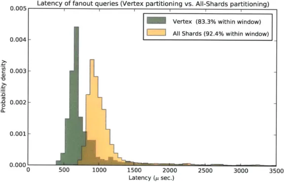
4-3 The two control strategies: vertex sharding and all-shards partitioning. Note the substantial fractions of data lying beyond the window range. See also Figure 4-4 . . . .

27 29 31 33 40 50 52 55

(7)

4-4 Comparing the two-tier strategy and the two control strategies on fanout latencies for synthetic graph and queries on the same synthetic workload as Figure 4-3 . . . . 56

4-5 Comparison of fanout query latencies of Two Tier and Vertex hash partitionings using real graph and logs . . . . 57

4-6 Comparison of intersection query latencies of Workload driven and Vertex hash partitionings using real graph and logs . . . . 58

(8)

List of Tables

2.1 Graph store usage statistics from query logs . . . . 2.2 Basic Twitter data . . . .

4.1 Comparison of latencies at different percentiles (in micro seconds) . .

4.2 Comparison of fanout latencies at different percentiles on real data (m usec) . . . .

4.3 Comparison of intersection latencies at different percentiles on real data (m u sec) . . . . 25 29 54 57 58

(9)

Introduction

Twitter is a popular web service and social network that anyone can join. Once in it, users create a profile and follow other users. Users can post brief messages, known as Tweets, that get delivered in real time to their followers. Similarly, users can view the latest messages from the users they follow.

As the network has grown to hundreds of millions of users, the backend systems supporting Twitter have developed into a vast custom infrastructure, offering many exciting opportunities for computer systems research. In particular, the data stores are responsible for storing all the user data as well as serving it quickly upon request. These services need to reliably store billions of relations between users, their profiles, their messages, and are tasked with serving this information fast enough to support the almost instant delivery of up to 30000 unique Tweets per second [10] to up to about 20 million users in some cases. This kind of scaling requirement is a strong motivation to seek alternative methods of serving these specific workloads.

The data stores, or data services in Twitter parlance, are among the core backend systems supporting the site. One of these data services, the graph store, is in charge of storing the relations between users. The graph store supports basic graph data structure operations such as inserting and removing vertices and edges, and retrieving adjacency lists for vertices. In addition to that, it also supports more complicated set arithmetic queries such as intersections, counts and differences. This thesis proposes improvements to the graph store.

(10)

for general purpose database systems, but these techniques generalize to other social network type workloads. Social network type workloads are characterized for their extremes. For example, in Twitter some users are much more popular and central to the rest of the community than others. Operations on them benefit from being treated differently.

In chapter 1 I survey the general purpose partitioning approaches used in other systems and how they related to query. In chapter 2 I look at the specifics to Twitter's workload. Knowing the specifics of both the kind of data stored by Twitter's graph store and the patters in its query workload help motivate proposals to improve the specific Twitter case. In chapter 3 I introduce the two proposals and quantitative arguments to explain why they should work. Finally, in chapter 4 I present the results from prototyping and benchmarking these techniques on both synthetic and real data provided by Twitter.

(11)

Chapter 1 Background

Many systems with high throughput needs such as Google, Facebook or Twitter achieve their scalability goals by building distributed infrastructure. This is the case for most of their infrastructure, from the web servers and caches down to the databases backing these services. In the specific case of databases, the potential gains from using multiple computers simultaneously depend partly on a good partitioning of the underlying data. Database partitioning in general is a widely studied topic, and there are several standard solutions that work well in general but are not optimal in the specific case of social network workloads. This thesis presents and evaluates two different partitioning strategies for social network type workloads.

There are two basic properties desirable from shared nothing distributed system. The first property, scale out, is that we can double the throughput of the system simply by doubling the number of nodes, without affecting latency. The second property, speed up, is that we can halve the latency by doubling the number of nodes. In practice, it is common that doubling the number of nodes in a system will less than double its throughput, or less than halve the latency according to the objective, but those are still the ideals. For websites such as Twitter scale out is seen as the primary goal because it implies that an increase in users can be matched by a proportional investment in machines, and that the average cost of running the site remains the

(12)

same. Latency is also important from the user experience perspective: the web page needs to feel responsive, and messages sent from user to user should arrive almost instantaneously.

Traditionally, workloads fall into two categories. The first category is online trans-action processing, or OLTP, in which the read and write sets of an operation are fairly small. The second category is online analytical processing, or OLAP, in which the read sets are fairly large. The emphasis on the first category is on ensuring scale out, while for the second category there is also attention to speed up. Very often, the databases serving websites are considered OLTP, and optimized for throughput. But because in social networks such as Twitter some users have a lot more edges than others, then for such users, queries like counts and scans are in fact a lot more similar to OLAP. This type of extreme workload variation is one of the key differences from other typical workloads, and why speeding up some of the queries becomes impor-tant. In the next section we wee how different data partitioning policies influence a system's scaling properties.

1.1 Database partitioning

Ideally, a partitioning strategy enables scaling by distributing all work evenly across the nodes and having each node work independently of the others. When the work is not evenly distributed among nodes then the overloaded nodes will likely show reduced throughput, thus reducing overall system throughput. There are reasons why work may not be perfectly distributed, one is the unpredictability of which items will be popular. Similarly, communication and coordination across nodes mean there will always be some degree of dependence between nodes. When the nodes need to constantly communicate data or coordinate updates to ensure they are all or none, like in distributed transaction, then the extra waiting due to locks may reduce throughput. Even if there is no locking, all the communication between nodes may turn network bandwidth into the bottleneck. Some operations invariably require looking at several

(13)

tuples at the same time, and these may be located in different physical computers. The most general purpose partitioning strategies are hash and range partitioning

[6].

Like their name suggests, hash partitioning uses a hash function to map rows to nodes, while range partitioning defines value ranges and then maps each to a node. Given an suitable hash function, hash based partitioning on any sufficiently diverse attribute will achieve the goal of balancing tuples and requests evenly, even as the table changes. On the other hand, hash partitioning only guarantees to map equal values to equal nodes. Two different values will be mapped to the same machine only

by chance no matter how similar. With probability 1/n for a cluster of n machines,

which tends to 0 as n grows. Range partitioning, on the other hand, will map rows with values close in their natural ordering to the same machine, achieving locality. Range partitioning may spread things less equally than hashing and will need to repartition in case one range turns out to be a lot more popular than other ranges, but its locality properties may help reduce the competing cost of communication across nodes when queries themselves tend to read nearby values of attributes. This thesis proposes two alternative partitioning methods that are not intended to general purpose, but that should work better for Twitter graph store workloads, explained in more detail in chapter 2.

We saw what methods we can use to partition, but another aspect of partitioning is which attributes we decided to partition by. Parallel joins are a typical example. If two large tables are expected to be joined regularly on a field x, partitioning both ta-bles using the same policy on field x allows the join to proceed in parallel without need to reshuffle one of the tables across machines. In this case, there is both a through-put gain (no communication) and a latency gain (parallelism). Another example illustrates the interactions between choosing partitioning attributes and partitioning methods. If we partition a table of log entries by using timestamps and a range par-titioner, then only one machine will be in charge of receiving all updates at one time and can be overloaded. On the other hand, if we choose to partition by a hash on the timestamp the write load would be spread across the whole cluster.Similarly, if we

(14)

had chosen to partition by a range on a different attribute such as log even category, we would also more likely have spread the workload. The moral is the partitioning decisions need to be made based on knowledge of the workload.

The closely related concept of database replication deals with how many copies of each block of data to keep and where to keep them. Even though replication is often used primarily to ensure fault tolerance, replication decisions also can help improve performance. For example, a system may replicate heavily read data, allowing the read requests to be served by different machines. On the other hand this replication policy increases the cost of writing an update. Depending on the read to write ratio of the data, this policy can increase or decrease throughput. Another example of using replication for performance purposes is when a database replicates a table thats frequently joined with others, this policy helps avoid communication overhead, and again, involves changing the cost for updates. In this thesis, the aim was to not affect writing overhead, so we do not consider alternative replication policies, mostly focusing on the partitioning itself.

Different partitioning policies involve two different implementation challenges. The first challenge is in storing enough information to enable efficient lookups. Hash partitioning is very practical from this point of view, because a hash function contains all the information needed to map any tuple to its location, the overhead for both storage space and lookup time is 0(1) relative to the number of tuples in the database as well as the number of nodes, this is relatively little state, so we could even place it in the client library directly. Range partitioning is not as easy, it involves keeping a range directory structure that grows as 0(r) where r is the number of ranges we have split the tuple universe into, because of that, it is less practical to place the state in the client library and we may need a partition manager node in the archi-tecture. Alternative partitioning systems, such as those proposed in this thesis, also need their own customized data structures for implementation. The storage challenge is complicated by system needs to scale up and tolerate node failures, which is the second challenge.

(15)

The more nodes participate in a database, the more likely it is some will fail, and also the more we need to support easy addition and removal of nodes. The partitioning infrastructure must make it possible to add new nodes without creating too much work to adapt. For example, if our partitioning function were f(k) = hash(k) mod n where n is the number of nodes, then the load would be well balanced on a static system. On the other hand, if n changes then the system must move most of the data from from their old location to the new one. There are more elaborate techniques to deal with these problems, such as extensible hashing and consistent hashing, but they are more complicated than in the static case. Consistent hashing, for example, requires an ordered list of size 0(n) where n is the number of nodes. It also requires to be updated whenever there is an event such as a node leaving or entering the system. In addition to dealing with nodes that enter or leave the system, range partitioning must react to many tuples entering or leaving the same range, and react by splitting or merging ranges and relocating data accordingly. As routing information grows, the system needs to be able to recover it after failures and to keep it consistent across different servers and between servers and actual nodes storing the data. All of these are important problems, but not the focus of this thesis.

1.2 Graph oriented systems

In section 1.1 I described partitioning from the general point of view of databases. This thesis is specifically concerned with partitioning policies for the Twitter graph store. The graph store does fall within the domain of databases, but has a more specific interface and workload. In the case of the graph store, the data is users and their relations, and the operations are adding users and relationships between users, and reading them too. I explain the interface and workload in more detail in

chapter 2.

Graph workloads are a specific niche of database workloads, but they are not unique to Twitter nor to social networking applications. Geographic entities such as

(16)

roads and cities, semantic web relations and graphical models in machine learning all exhibit graph structure and can be processed as such. Similarly, Twitter's graph store is not the only one graph data store. There are many other systems specifically designed to store and process graph data. Ultimately, a graph can be stored in a typical relational database and queried there, too. For example, we can store a tables of vertices and tables of edges. Operations such as neighbors, queries such as degree per nodes, 2-hop neighbors can be expressed etc can all be expressed with typical SQL statements. Nevertheless, graph systems with custom interfaces and organization are becoming popular [24] [31].

The graph processing systems described can be split broadly into two categories: analytics and storage. Graphlab [21], Pregel [22], and Cassovary [16] work for the analytics category. Graphlab and Pregel are distributed, and Cassovary is not. All of them offer a graph-centric programming model and aim to enable efficient execution of richer algorithms. On the other end there are the storage systems, these include the Twitter graph store (also known as FlockDB)[17], which provides distributed and persistent storage with online reads and writes and offers a much more limited interface: get sets of neighbors, get edge information for a specific edge and a few basic set operations. Other stores such as Neo4j sit somewhere in the middle: Neo4j offers persistence, online updates and a richer interface for queries: shortest paths, 2-hop neighbors, etc, but is not distributed [24].

Finally, partitioning in graph oriented systems is done similarly to that of databases. Pregel uses a function of the hash(ID) mod N as the default partitioner, for example, but allows to plug in different partitioners [22]. Apache Giraph is similar [3].

1.3 The abstract partitioning problem

I have introduced the partitioning problem in databases, why it is relevant to graph

(17)

partitioning in the Twitter graph store, it is worth noting that the partitioning prob-lem is complex algorithmic probprob-lem for which no solution is known. Partitioning problems, even in offline batches are often hard to solve optimally. Here I present two

NP complete problems that show, in one way or another, that balancing problems

can only be dealt with heuristically. The first problem is about partitioning a set of numbers of different values, the second problem is about partitioning a graph with arbitrary edges.

Definition 1. Balanced partition problem. input A group of n positive numbers

S = a1, ...a,

output A partition of the numbers into two groups A and S A such that | ZaA

a-Zap aj is minimized.

This problem can be interpreted as a way to optimally balance the load across servers if we knew ahead of time the load ai for each task. In that case, a scheduler could run the algorithm and then allocate tasks accordingly. One interesting aspect of this problem is that it involves no communication among the parts, but already is NP-complete. For practical purposes, there exist several quick heuristic methods to generate a (non necessarily optimal) solution to this problem.

Often, data partitioning problems also need to consider communication costs. If doing task a1 and a2 involves some sort of communication, then we may want to

group them in the same partition. Problems like such as this one, with an added communication cost can be better modeled as the graph partitioning problems rather than set partition problems. Formally speaking, the graph partitioning problem is the following.

Definition 2. Graph partition problem input A graph G = (V, E), and targets k and

m.

output A partitioning of V with none of the the parts is larger than |V|/m and

(18)

The graph partitioning problem, unlike the balanced partitioning problem, does not necessarily have weights, nevertheless it is NP-complete. A more general version allows both vertex and edge weights is therefore just as hard. Like for the number partition problem, there are efficient (but, again, not necessarily optimal) heuristics to solve it. One such heuristic is the Kernighan-Lin method that try finding a good

solution in O(n2_{lgn) time [19]. Kernighan Lin is also one of the components of the} more general METIS heuristic [25]. METIS is an algorithm and associated implemen-tations that aims to solve larger scale instances of these problems. Graph partitioning algorithms such as these have been used for parallel computing applications as a pre-processing step, to divide the load evenly among processors.

The problems and heuristics presented in this section were results on the static (see everything at once, and graph does not change) case. One challenge for these algorithms is to scale to larger graphs. As the input graph size increase it may no longer be possible to fit the graph in a single machine. Another challenge for graphs that are constantly changing is to compute an incremental repartitioning that does not move too much data across parts and yet is effective. Running a static partitioner periodically may not be a good solution if the algorithm produces widely different partitions every time. Despite the challenges, there exist heuristics for distributed streaming graph partitioning [28].

Even though the partitioning problem is hard, a partitioning strategy does not need to achieve optimality. In the previous subsections we saw that hash partitioning is widely used despite causing many edges to cross between parts, so many other heuristics will probably perform better. For this thesis, one of the strategies proposed makes use of the METIS algorithm.

In this chapter I explained the relation between partitioning and scaling, listed the typical partitioning strategies supported by databases and their more recent relatives known as graph processing systems, and described known hardness results that are relevant to the partitioning problem. The next chapter will expand on the Twitter specific aspects of the project.

(19)

Chapter 2 Twitter specific background

The main persistent Twitter objects are users, their Tweets, and their relations (known as Follows) to other users. Each of these objects has associated informa-tion such as user profile picture and locainforma-tion in the case of an individual user, Tweet timestamp and location for a Tweet, and the creation time of a Follow between two users. Any user can choose follow any other user freely, there is no hard limit. Con-versely, a user can be followed by anyone who chooses to. That policy combined with the growth in Twitter's popularity made some users such as the singer @ladygaga or current US president @BarackObama very popular. Each of them has about 20 million followers as of mid 2012. A note on terminology: Twitter usernames are com-monly with the '@' symbol. Also, by Followers of AA we mean all users @B such that @B Follows @A. Conversely, the term Follows of @A refers to all the users AC such that @A Follows @C. A user chooses her Follows, but not her Followers. The relation is asymmetric.

Each Twitter user gets a view of the latest Tweets from his Follows, this view is called his Timeline. If @A Follows @B and ©B Tweets c, then @A should see c in its timeline. Constructing all users' Timelines is equivalent joining the Follows table with Tweets table. At Twitter, the three tables: User, Tweet and Follows are implemented as three different services. So we talk about each table as the User store,

(20)

the Tweet store, and the Graph store respectively. These databases are constantly joining entries to construct timelines, so all the operations involved in these process are crucial to Twitter's functioning. This separation also impacts the amount of user information available internally to the graph store, for example, it is not possible to simply partition users by country or by language because this information is not really part of the graph store, which deals with users only as user ids.

A second note on terminology: since the the graph vertices correspond to users,

we treat the term vertex; and user as synonyms. Similarly, a Follow relation and an edge are also synonyms. The term 'node' is reserved for the physical machines on which the system runs.

2.1 Graph store interface

For the purposes of this thesis, we can think of the graph store as a system supporting three kinds of updates and three kinds of queries. The updates are to create an edge or vertex, to delete an edge or vertex and to update an existing edge. The three queries are described below. In short, the graph store can be thought of as offering basic adjacency list functionality, with additional support for some edge filtering and intersection.

The first basic query, known as an edge query, is a lookup of edge metadata given the two edge endpoints. Metadata includes timestamps for when the edge was created, when it was last updated and other edge properties such as the type of the edge. For example, it could be a standard 'Follow', or a 'Follow via SMS' that specifies SMS delivery of Tweets, or a 'blocked' edge. Edges are directed. At the application level, the edge query enables the site to inform a visitor of its relation to the profile he's looking. In the case of blocked users, the metadata also enables the system to hold their Tweets from being delivered to the blocker.

(21)

referred to as a fanout query. A fanout query returns all the neighbors of a given vertex @A. The complete interface to the graph store allows for some filters to be applied before returning results. For example, we may wish to read all the Followers of

OA, or all the Follows of A or users blocked by @A. Some of these queries may involve

filtering out of elements. The fanout query interface also offers to page through the results of a query, useful in case the client is not prepared to deal with large result sets, or simply because may be interested only in 1 or 10 followers. Such queries are used for display in the profile web page, for example. The paging interface requires specifying both a page size for the result set and an offset from which to resume. The ordering of the result set can be set to be the order in which follows happened. This provides a way to answer queries like 'who are the 10 latest followers?'. Because the time ordering of the edges probably differs from the natural order of the user ids, some of these queries involve more work than others. The most important use case of fanout operation is Tweet routing and delivery. Whenever user AA Tweets, the effects of that action must be propagated to the followers returned, which we find out using a fanout query.

The third query is the intersection query, the intersection of neighbors for two given vertices. Intersection queries are more heavy weight than fanout queries. A single intersection operation implies at least two fanout type operations plus the added work to intersect the results. The extra work can be substantial, for example if the two fanouts are coming from separate machines and the are not sorted by user id to start with. One design option is to let the server implement only fanout queries, and have the clients intersect the results themselves. This approach reduces work at the server, but increases external bandwidth use to transmit results that eventually get filtered anyway. Like with fanout queries, there are many parameter variations on this query. Like with fanouts, the result for an intersection can be paginated.

There are several Twitter use cases for the intersection query. When a user @A visits @B, the website shows AA a short list of his Follows that in turn are Followers of @B. This is an intersection query of the Follows of @A and the Followers of @B.

(22)

Because the website only displays the first 5 or 10 names, this use case only requires a executing part of the full intersection. The most important Twitter use case of the full intersection is, like with fanouts, also related to Tweet routing. When a public conversation takes place between two users AA and AB, Twitter propagates the conversation only to Followers of both @A and @B, so it must intersect Followers of

@A with Followers of AB. There are potentially many uses for intersection query, such

as computing a similarity metric between users such as cosine similarity, or measure the strength of the connection between two users @A and @B by intersecting AA's Follows with @B's Followers and counting the result. Another example is in listing paths: a full intersection of @A's Follows with @B's followers encodes all the 2-hop paths from @A to @B. An intersection query could also be used for looking more complicated path patterns in the graph, like follow triangles. or simple statistics: for example, how many mutual Follows-Followers does @A have? We can answer this by intersecting Follows @A with Followers @A. Intersection is the more complex operation considered in this thesis, and given these use cases it is possible that gains from improving its performance may enable the graph store to handle more interesting queries.

The graph store interface supports more than fanout and intersection queries. It actually supports more complicated set arithmetic such as three way intersections, and set differences. It also allows counting queries. A general optimization strategy for general set arithmetic queries is out of the scope of this thesis, and we will see that empirically the main uses of the store are fanouts and intersections.

There is limited need to enable arbitrarily powerful queries in the graph store be-cause Twitter has also developed a separate graph processing system called Cassovary (mentioned in chapter 1). At Twitter, Cassovary is used for more analytic workloads. Unlike the graph store, Cassovary loads data once and then mostly reads. Because of the read only workload, data can be compressed much more. Because it is not meant to be persistent, all of it can be stored in memory. Even at the scale of Twitter's operations, the graph in compact form can fit into a single machine. As an estimate,

(23)

the connections between 1/2 billion users with a combined degree of 50 can be rep-resented efficiently in around 100GB. The kinds of queries done in Cassovary include things like page rank and graph traversal, and it is used to power applications such as Follow recommendations, similarity comparisons between users and search. These operations can use data that is a bit stale, since they are not meant to be exact. By contrast, the graph store cannot fall behind updates. When a user follows another, this change should be reflected in the website immediately. New Tweets from the re-cently followed user should be delivered as soon as there is a subscription. Similarly, when a user blocks another the system should react immediately. This is not the case with recommendations, which can be computed offline and more slowly.

Both FlockDB and Cassovary are open source projects, so full details of their interfaces and current implementations are available in the source repositories [17]

[16]. While the interface description tells us which operations are possible, viewing

actual logs informs us of which is the actual use the system. The next sections profiles the queries and data stored in the system..

2.2 Workload profile

The graph store workload is made up of a mix of the queries for edges, fanouts and intersections as well as by the data stored in it. By checking operation frequencies we gain a clearer picture of how the API is really used: which operations are relevant and which are not. And looking at the graph itself we understand the variations in work needed by these operations. This section clarifies the workload and helps understand what a social network workload is like.

The goals of analyzing the workload are to check that the operations merit opti-mization, to learn about the average and extreme cases, and to possibly learn facts that may help us devise improvements.

(24)

and intersections to the load on the graph store?

2. Are queries are made evenly across users or not? Are there any users with many fanout queries? Are there users that are intersected often?

3. Are users that get queried for fanout often also queried for intersection often?

4. What is the distribution of data among users? We know some users have reached 20 million followers while others have only about 50, are there many such cases? can these large follower counts be considered outliers or are there too many of them?

5. Is there any relation between a user's query popularity its degree?

To answer these questions I used a sample of all incoming requests to the running graph store for a few hours, resulting in about 300 million samples as well as a sepa-rately collected snapshot of the Follows graph. These logs did not sample operations such as writes, deletes and updates, nor counting operations, so we are limited to only comparing among queries.

2.2.1 Query profile

The short answer to the question about the frequencies of the different operations is that fanouts are the most popular queries, comprising about 80% of all queries. As described in section 2.1, the graph store supports paginated results for fanout queries, and so it accepts both a page size and an offset as part of the fanout query arguments.

By analyzing the more common page sizes and offsets, I found that the main form of

fanout query is only querying for a small page size starting at offset zero. The second most popular fanout query also starts at offset zero, but requests page sizes of above

100. As described in section 2.1 small page size fanout queries may be produced by

user page views. Fanouts done with larger page sizes are more consistent with the Tweet routing use case. The full aggregate results are shown in Table 2.1.

(25)

operation type frequency fanout (small page, zero offset) 70% fanout (large page, zero offset) 10%

intersection 1.5%

edge metadata 0.5%

other fanouts, etc 18%

Table 2.1: Graph store usage statistics from query logs

The 'other fanouts, etc' category includes fanouts done at starting at larger offsets and a few unrelated operations. Because a full logical fanout query may be actually implemented as a series of paged requests at different offsets, the 'other fanouts, etc' category may include the same logical fanout repeatedly, which is why I show it separately. And about the other queries, intersections happen much less often, suggesting they may not be as important. Surprisingly, edge metadata queries seem to happen seldom.

The significance of a particular type of query in the workload is not just a function of how frequent it is, but is really a product of its frequency and the load each individual operation places on the system. For instance, the page size given to a fanout query has a relation with the potential cost of the operation. Requesting the latest 1 or 10 followers is lightweight, but requesting 1000 of them can involve more work both in scanning it (it may occupy multiple pages on disk) and in sending it (its more data after all). For this reason, I believe they should be considered separately. Similarly, a single intersection operation implies at least 2 fanouts and at some merging (which can be quadratic in size). Even at small page sizes, the intersection operation may need to internally read much larger fractions of the fanouts in order to compute a small number of answer elements. so, the effect of intersection on system load could well be larger than its frequency alone suggests.

The effect of this load factor can easily match the effect of frequency: since the light weight fanout operations represent at most about 70% of the requests, and the heavy weight ones about 10%, then an individual heavyweight operation needs to be about 7x more work than a single light weight, for the heavyweight operations

(26)

become just as significant as the light weight ones. I did not have a way of checking whether this difference in workload is as significant as this or not. Either way, as a result of this observation the work in this thesis focuses on the heavy fanout queries and slightly less on the intersection queries, and none on the edge queries.

2.2.2 Query skew

The second question is whether queries are uniformly distributed across users. It is often the case in other systems that requests have certain skew. For example, in a news website it is expected the recent articles are probably requested much more than older ones. In Twitter's case, individual people may be much more active users than others, and some people's profiles may be much more visited than others. Information about query skew is important for optimizations. A large skew makes it harder to balance load across nodes easily, because even if the databases are nominally balanced

by user count, not all users contribute to system load the same way. On the other

hand, caching may be more effective in large situations than in the case uniform access, which means skew can also be helpful. Either way, a system that assumes a uniform distribution may not be capable of deal with extremes such as particularly popular users or messages. Because of its important effects, also many papers or benchmarks model this kind of skew explicitly by generating queries with some bias, for example [4] and [5].

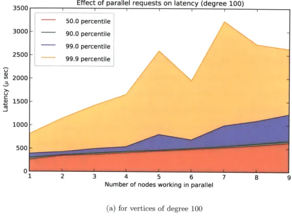
In order to verify whether this kind of query skew also occurs at Twitter, we ag-gregated the sample query logs by user and randomly re-sampled about 1000 different users, we got a view of the number of operations they were involved in. The results appear in Figure 2-1.

The plot is on a log-log scale because of the extreme values of the workload. From Figure 2-1 we can see that fanout skew is a lot larger than that for intersection, But in either fanout or intersection, the skew is large. While most vertices are involved in relatively few queries of either type, the most queried vertices are involved in up to

(27)

Rank plot for number of intersection

101 102

Rank

(a) Intersections look linear

Rank plot for number of fanout queries

101 102

Rank

(b) Fanouts show different behavior at two ranges

Figure 2-1: Frequency of different queries vs rank

102 C-C 0 I-0 E 101 100 1 0 100 103 0* C 4-0 E 103 102 101 100 L_ 100 103

(28)

slightly less than 10k fanout queries or up to about 100 intersections (recall this is a small sample of about 1000 vertices that appear in the query logs). Intersection for some reason shows a very straight line, typical of power law distributions, while the fanout frequency somehow is made up of two different straight line segments. These plots show skew results consistent with measurements seen in other workloads, such as Wikipedia [30]. The results for skew on both queries show that there are opportunities in caching, as well as in pursuing which users are the most actively queried and maybe treat them differently. Later in this chapter we check for whether these users also have large degrees, and find a weak but nevertheless positive correlation between these variables.

2.2.3 Query correlations

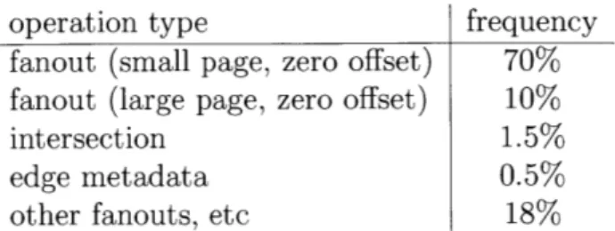
We saw that some users are queried much more than others. The third question is whether the same users that are popular for intersections are also popular for fanouts. In this section we see there is a weak but unambiguous correlation. The results of these measurements are shown in Figure 2-2.

Interestingly, fanout queries and intersection queries are observably correlated. This suggests that it is meaningful to think of a vertex as being 'popular' for queries as a whole, because being popular for some types of queries implies it is likely also popular for other kinds. Correlation of skews also implies the overall workload skew is more pronounced than if there was no correlation.

2.2.4 Graph data profile

The fourth question was not about the queries to the data store but about the data in it. As of March 2012, Twitter has an active user population of beyond 140 Million

[15], and the overall number of vertices is some multiple of that (though most of the

(29)

log-log scatter 10 4 . 103 E 02 0 . 101

plot of fanout involvement vs. intersection (corr: 0.532, log-corr: 0.491)

100

100 101 102

fanout involvement

Figure 2-2: log-log scatter plot showing the relation between fanout popularity and intersection popularity

For the experiments I performed, described more extensively in chapter 4 I worked with an older sample of the graph with 130 million vertices and an average follower count of 40, for a total of about 5 billion directed edges. The maximum degree vertex in this sample had about 1 million followers.

The basic Twitter data information is summarized in Table 2.2, side by side with the dataset I used for some of the benchmarks.

quantity

number of vertices

average followers (in-degree) max number of followers

number of edges (using average)

2012 estimates > 140 million < 100 24 million > 10 billion workload data 130 million 40 1 million 5 billion

Table 2.2: Basic Twitter data

In the snapshot, the gap between the average in-degree of 40 and the maximum in-degree of 1M is typical of of heavy tailed distributions. In Figure 2-3 A rank plot shows the in-degree as a function of rank. Like with many other naturally occurring

involvement * e.g

ft.

I I

II

.26

U U

I I..

*

~ I

S **

I,

.

3 33,

1

9, 0 S 0 'I

(30)

graphs, the degree distribution tail is similar to a power law: most of the users have relatively small degree but with a still substantial tail of users having larger degrees. Like with the plots for query skew shown Figure 2-1, the plot looks as a straight line in part of the range, and shows variation along orders of magnitude. From the smoothness of the line We can see how there is a natural progression in degree, which means heavy vertices cannot really be considered outliers because there is a clear progression from the bulk of the data to the extreme values. This suggests that any system needs to know how to deal with both very large and very small degree vertices, and it may need to do so differently. This is one of the motivations behind one optimization approach described in chapter 3.

Figure 2-3 again shows the wide range of both the out-degree and in-degree dis-tributions, but additionally also shows how they are very strongly correlated. This correlation holds even the in-degree is decided independently by other users whereas an individual user is in full control of his out-degree. Also note, the out-degree and in-degree are very correlated but an the out-degree is one order of magnitude smaller in range than the in-degree.

The differences between out degree and in degree have suggests interesting opti-mizations. For example, may be better off storing edge (a, b) as associated with a rather than with b, because this method reduces the incidence of extreme degree cases. Similarly, we could decide users pull Tweets rather than push them. Because pulling is an operation with load proportional to the out degree, whereas pushing is propor-tional to the in-degree, load may be more balanced this way. I do not pursue these ideas further, but they exemplify the kind of optimizations enabled by knowledge of

the specific workload 1.

(31)

Rank plot for Number of Followers

101 102

Rank

(a) The number of followers (in-degree) of a vertex

log-log scatter plot of number of follows vs. number of followers (corr: 0.357, log-corr: 0.757) 0

I

a e 0 0 0 10 1 e a 102 104 number of follows

(b) Strong correlation between in-degree and out-degree

Figure 2-3: rank plot of in-degrees over vertices in sample and correlation

without-106 10 5 10 4 0 10 U) 4--10 E z ₁₀₁ 100 1 100 103 106 105 14 L 104 0 0 0 10~ 101 10 0 10 105 I 10 3

(32)

2.2.5 Query-graph correlations

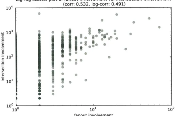
The last question is about correlations between query skew and degree skew. There are arguments why this correlation is plausible: perhaps heavy users are much more active by visiting the site or tweeting more often. Also, a vertex with very large degrees implies a larger historic amount of writes, and would seem more likely to be followed in the future. By joining the log records from section 2.2.1 with the graph snapshot, we checked for any significant patterns. The results are shown in Figure 2-4. The correlations are positive but fairly weak.

In this chapter I introduced the Twitter graph store and its API, including and the two main operations my thesis aims to improve; fanout and intersection queries. I also explained the relevance of these operations from the application's perspective. Most importantly, I presented statistics on actual usage, these included both information about which queries are more common, which turn out to be fanout queries of small page size followed by fanout queries of larger page size, and then by intersection. Also, I exhibited the heavy query and and degree skews in the query patterns and graph respectively, these observations form the basis of the optimization proposals presented in the next chapter.

(33)

log-log scatter plot of intersection involvement vs. (corr: 0.117, log-corr: 0.011) number of followers 106 105 1 04 10 02 4- 0 .0 E ₂ CM 102 101 100

(a) Intersections seem to be independent from degree

log-log scatter plot of fanout involvement vs. number of followers (corr: 0.571, log-corr: 0.197)

101

fanout involvement

(b) Fanouts are slightly related to degree

102

Figure 2-4: relation between query popularity and number of followers

0 't 0 0 0 00 GOW *00 10 101 102 103 intersection involvement 106 105 104 L103 0 4- 3 E e 102 101 10 0 * 0 0 * * 0 0 * gO . 60

Sg

0.e 100 10 4 0 L

(34)

Chapter 3 Optimizations

The contributions of this thesis are two different partitioning methods that improve fanout and intersection query performance. Performance refers to many desirable but different properties of a system. As discussed in the introduction, throughput is one such desirable property and it has a direct effect on the costs of growing system. The optimizations aim to improve latency for individual requests. Specifically, the objective of these techniques is to improve service latency, without sacrificing anything at all levels of the distribution, in other words, improving the worst cases without worsening the common case.

There are two good reasons for reasoning about latency in terms of distributions rather than as a single number. The first reason is that if a distribution has a very large spread the mean value is less meaningful. So for instance in the case of Twitter the degree of all users in itself shows high variance, as does the rate at which some users are queried. In situations such as these, average case analysis fails to account for the significant mass concentrated at the extreme cases. A second reason for targeting the full latency distribution rather than only median or average cases is that large latency variability for a service (even with good expected case) creates latency problems when integrating that system into larger ones. The intuitive argument is that when call latency is variable, parallel call latency worsens as we add

(35)

more calls. In this thesis this same phenomenon affects the design of a partitioning strategy internally later on in this Chapter, in subsection 3.1.2. Perhaps as a result of these reasons it is common practice in service oriented architectures to include latency targets such as bounds on latency at the 99.9 percentile [9].

Another important decision in searching for better partitioning strategies was to exclude adding replication. A few optimization proposals in the literature often involve exploiting not only partitioning but also replication

[30].

While those opti-mizations will likely improve read performance, they involve trading reads off against writes. Writes are one of the core differentiators of the graph store, so there was a conscious effort to focus on improving the reading queries without modifying write costs.

From the information in the previous chapter we know that there are significant degree and query skews. Degree skew causes longer latencies in fanout queries because some vertices simply have very large degrees. The first optimization approach in this chapter reduces the effect of degree skew by making fine grained partitioning decisions for the tail of the degree distribution. The result is a corresponding improvement in the latency distribution. Query skews mean that some queries are more popular than others, this applies also to pairs of vertices involved intersection queries. The second proposed optimization partitions vertices according to how often they are intersected so that they are placed in the same locations, yet, still are spread out so that no only one machine is overloaded. Both of these optimizations are made possible partially because we can make these more fine grained partitioning decisions only of the more significant or active parts of the graph. I expand on the techniques and their motivation in the next sections.

(36)

3.1 Optimizing fanout queries

Under the current hash by vertex approach employed in the Twitter graph store, some fanout queries take much longer than others because some vertices have many more edges than others. Because we partition by vertex, then all edges adjacent to the same vertex will always be on the same machines. As new vertices are added to the graph and new edges connect old or new vertices, the differences in vertex degree will become more pronounced. For these two reaons, fanout query latency may become a problem.

Consider that the largest Twitter users have around 25 million followers at the moment of writing. Using conventional hardware parameters, we can estimate the minimum amount of time that different basic tasks take to execute on a vertex of degree 25M. Consider the time it takes to scan sequentially and in memory all of the fanout a heavy user of that degree:

8B 250musec lmsec

25M id x- id MB ~50msec

id MB 1000musec

So, assuming it takes 250 micro seconds to read 1MB sequentially from memory, it

would take 50 milliseconds to complete the task. This number is large enough to fall within the grasp of human perception. As a second example, consider the same task of reading 25M user ids but this time when done over the network or from disk. In that case the calculation changes slightly, and we get

8B 10msec 1sec

25M id x - x x ~ 2sec id MB 1000 msec

So, to read list of followers sequentially from Disk or to send them sequentially to

one node over Gigabit ethernet it takes about 2 seconds. This number is also over optimistic, it assumes we can make use of the full bandwidth, which is not the case if there are any seeks in disk for example.

(37)

reality other factors make these calculations fall far below what they actually are. For example, any extra information besides the user ids sent over the wire, or less locality in reads from memory, or paging through the result, would increase the time substantially. From a user standpoint, a difference of less than 5 seconds probably does not detract from the real-time feel of the experience but longer differences could. The graph store is only one of the many components that contribute to the latency between a tweet being posted by a user and the tweet being delivered to the last recipient, but its latency contribution grows with the number of edges in the graph, whereas some other contributors are independent of this latency.

Besides the previous latency argument, there are other reasons to improve fanout performance. There exist several side effects to having some users get Tweets delivered much later than others. One effect is that it causes chains of dependent tweets to stall. Many Tweets are responses or retweets of other tweets. Because delivering out of order conversations would be detrimental to user experience, Twitter implements mechanisms to enforce ordering constraints. One such mechanism is to withhold tweets from delivery until all of their dependencies have been satisfied, or to pull the dependencies upon discovering they are not satisfied. Any unsuccessful attempts to deliver a tweet or repeated calls to pull are a waste of bandwidth. The chances of long chains of stalled tweets increase as latency for large fanouts increases.

Having established the need for methods to improve fanout query latency, we turn to considering methods for improving it. Using parallelism to reduce latency as vertex degrees increase is a natural solution, but the more naive parallelization approaches do not work well. For example, one possible solution is to partition the edges for every vertex into 2 shards. This technique effectively slows the degree growth rate of the graph. Another possible approach is to instead of hashing by vertex, we hash

by edge. This way, all large degree vertices are distributed evenly across all cluster

nodes. The problem with this approach is that every query will require communication with all nodes, even queries for small degree vertices that only have a few followers will need to communicate with many nodes. The problem with both the hash by

(38)

edge technique and hash into two parts technique is that for a great fraction of the vertices, splitting their edges into two separate locations does not improve latency and moreover, needing to query all or many shards is a waste in bandwidth. Many vertices in the graph are actually of small degree, so it is quite likely that the overall system will be slower and have lower capacity than one partitioned using vertex hash. In order to evaluate what the optimal policy for partitioning edges is in view of the factors of parallelism and communication, I present a simple performance model for fanout queries in the following subsections, and I use it derive the 'Two-Tier' hash partitioning technique, the first of the two partitioning methods proposed in this thesis.

3.1.1 Modelling fanout performance

Intuitively, the main determining factor for fanout query latencies is the number of vertices needing to be read from disk or memory and then sent over the network, this cost is proportional the degree of the queried vertex, which we denote d. If we decide to parallelize, then the amount of work to do per node decreases, but the effects of variability network communication times start becoming comes in as a second determining factor. The more parallel requests there are, the more latency there is in waiting for the last request to finish. Equation 3.1 expresses the tradeoff between parallelism and parallel request latency more formally:

L(d, n) = an + max'(Li + qd/n) (3.1)

In Equation 3.1 a and q are system dependent constants, d stands the vertex degree and n for the number of nodes involved in the query. When the n parallel requests get sent to the n nodes, each of those n nodes performs an amount of work proportional to the amount of data it stores, d/n. The initial term an corresponds to a client

(39)

side overhead in initiating the n requests1 . Additionally, a random delay Li is added independently to each request, representing latency variability. The total latency

L(d, n) is a random variable, because the Li are assumed to be random as well.

Since we are interested in optimizing latency for an arbitrary percentile level p, let percentile(p, X) stand for the pth percentile of a random variable X. For instance, percentile(O.5, X) is the median of a distribution.

3.1.2 The cost of parallel requests

The formula in Equation 3.1 also captures, indirectly, what happens as we increase the n. Whenever we parallelize an execution we potentially reduce the work term d/n done at each node, but add the overhead of making more calls. This overhead has several sources: making each call involves some work, so as we increase the number of calls this work overhead increases linearly with it. Depending on the amount of work we are parallelizing in the first place, this call overhead may become important for large enough n. This overhead is also described elsewhere [12]. A second factor is in the variability of the time it takes to make these function calls. Each call made over a network has a natural variability in latency. Since ultimately we need to wait for the last of the parallel calls to finish, we need to wait for the worst case of n requests. As n increases, the chance of delay also increases.

In this section I explore the sorts of overheads that can occur via simulation. It is reasonable to assume that the effect of making a parallel call to an extra machine will slow the system down a bit, but the exact functional form depends on the variability distribution in the first place. A few simulations show what the effect on latency is like for three different popular distributions: exponential, Pareto (also called a power law) and uniform. As we increase the number of nodes we get the trends in Figure 3-1. Note that the effects can go from seemingly linear, like in the case of the Pareto distribution, to very sublinear like the case of the exponential. In empirical tests

'Though technically, this cost itself may be lowered to ig n if the initialization of requests is itself done in parallel

(40)

Parallel (exponential distributed) requests and latency

>1

5 10 15

Number of nodes working in parallel

Parallel (pareto distributed) requests and latency

5 10 15

Number of nodes working In parallel

Parallel (uniform distributed) requests and latency

C

5 10 15

Number of nodes working in parallel

Figure 3-1: Simulated effects of increasing the number of parallel requests on latency for different types of delay distributions (at 50th, 90th, 99th and 99.9th percentiles)

Database partitioning strategies for social network data