A Bayesian dose finding design for clinical trials combining a cytotoxic agent with a molecularly targeted agent

(1)

HAL Id: hal-01298649

https://hal.sorbonne-universite.fr/hal-01298649

Submitted on 6 Apr 2016

HAL is a multi-disciplinary open access

archive for the deposit and dissemination of

sci-entific research documents, whether they are

pub-lished or not. The documents may come from

teaching and research institutions in France or

abroad, or from public or private research centers.

L’archive ouverte pluridisciplinaire HAL, est

destinée au dépôt et à la diffusion de documents

scientifiques de niveau recherche, publiés ou non,

émanant des établissements d’enseignement et de

recherche français ou étrangers, des laboratoires

publics ou privés.

A Bayesian dose finding design for clinical trials

combining a cytotoxic agent with a molecularly targeted

agent

M.-K. Riviere, Y. Yuan, F. Dubois, Sarah Zohar

To cite this version:

M.-K. Riviere, Y. Yuan, F. Dubois, Sarah Zohar. A Bayesian dose finding design for clinical trials

combining a cytotoxic agent with a molecularly targeted agent. Journal of the Statistical Society of

London, JSTOR, 2015, 64 (1), pp.215-229. �10.1111/rssc.12072�. �hal-01298649�

(2)

A Bayesian Dose-finding Design for Clinical Trials

Com-bining a Cytotoxic Agent with a Molecularly Targeted

Agent

M-K. Riviere

INSERM, UMRS 1138, Team 22, Centre de Recherche des Cordeliers, Universit ´e Paris 5, Universit ´e Paris 6, Paris, France

IRIS (Institut de Recherches Internationales Servier), Suresnes, France

Y. Yuan

Department of Biostatistics, The University of Texas MD Anderson Cancer Center, Houston, TX 77030, U.S.A.

F. Dubois

IRIS (Institut de Recherches Internationales Servier), Suresnes, France

S. Zohar

INSERM, UMRS 1138, Team 22, Centre de Recherche des Cordeliers, Universit ´e Paris 5, Universit ´e Paris 6, Paris, France

Abstract. Novel molecularly targeted agents (MTAs) have emerged as valuable alternatives or complements to traditional cytotoxic agents in the treatment of cancer. Clinicians are com-bining cytotoxic agents with MTAs in a single trial to achieve treatment synergism and better patient outcomes. An important feature of such combinational trials is that, unlike the efficacy of the cytotoxic agent, that of the MTA may initially increase at low dose levels and then ap-proximately plateau at higher dose levels as MTA saturation levels are reached. Therefore, the goal of the trial is to find the optimal dose combination that yields the highest efficacy with the lowest toxicity and meanwhile satisfies a certain safety requirement. We propose a Bayesian phase I/II design to find the optimal dose combination. We model toxicity using a logistic re-gression and propose a novel proportional hazard model for efficacy, which accounts for the plateau in the MTA dose-efficacy curve. We evaluate the operating characteristics of the pro-posed design through simulation studies under various practical scenarios. The results show that the proposed design performs well and selects the optimal dose combination with high probability.

Address for correspondence: Sarah Zohar, INSERM, UMRS 1138, Team 22, Centre de Recherche

des Cordeliers, Universit´e Paris 5, Universit´e Paris 6, Paris, France. Email: sarah.zohar@inserm.fr; and Ying Yuan, Department of Biostatistics, The University of Texas M. D. Anderson Cancer Center, Houston, TX 77030, USA. Email: yyuan@mdanderson.org

(3)

1. Introduction

Traditional cytotoxic agents have played important roles in combating cancer. However, after decades of research, it has become difficult to find new cytotoxic agents that are sub-stantially more effective than the existing therapeutic strategies. Recently, novel molecularly targeted agents (MTAs), such as small molecules or monoclonal antibodies, have emerged as alternatives or complements to cytotoxic agents for treating cancer (Le Tourneau et al., 2010, 2011, 2012; Postel-Vinay et al., 2009). Unlike cytotoxic agents, MTAs modulate spe-cific aberrant pathways in cancer cells, while sparing normal tissue. To take advantage of both types of treatment agents, clinicians are exploring the possibility of combining tradi-tional cytotoxic agents with novel MTAs to achieve treatment synergism and better patient response.

This new trend of combining cytotoxic agents with MTAs for treating cancer brings new challenges for early-phase dose-finding trial design. These challenges arise from the differ-ence in the dose-efficacy curves between the two types of treatment agents. For cytotoxic agents, more is better (i.e., a higher dose yields a greater response) until a dose-limiting toxicity level is reached. However, the dose-efficacy relationship of the MTA may not follow a monotonic pattern: the efficacy of the MTA often increases at low dose levels and then plateaus (or approximately plateaus) at higher dose levels once a saturation level in the body is reached (Le Tourneau et al., 2010; Hoering et al., 2011). Although it is possible that efficacy decreases at higher dose levels, here we focus on the case in which efficacy first increases and then plateaus because such a dose-efficacy relationship is much more commonly encountered in practice.

Consequently, the conventional dose-ﬁnding paradigm of searching for the maximum tolerated dose (MTD) is not suitable for combinational trials of a cytotoxic agent with an

(4)

MTA, and it is imperative to consider efficacy and toxicity simultaneously, with the goal of finding the molecularly targeted optimal dose combination (ODC). This is because once the MTA dose-efficacy curve reaches a plateau, further increases in the dose of the targeted agent will not yield any therapeutic benefit, but will potentially result in greater toxicity (Postel-Vinay et al., 2009). In this article, the ODC is defined as the most efficacious dose combination that yields the lowest toxicity. As the lowest toxicity can still be excessive, we also require the ODC to satisfy a certain safety requirement, e.g., the toxicity probability must be lower than a certain upper bound.

Numerous designs have been proposed to find the MTD for trials combining multiple cytotoxic agents, without considering the efficacy endpoint. For example, Thall et al. (2003) developed a Bayesian approach to identify an entire toxicity “contour” of drug combina-tions. Conaway et al. (2004) proposed a dose-finding method based on the simple and partial orders of drug combinations. Yuan and Yin (2008) proposed a sequential dose-finding design that allows single-agent dose-dose-finding methods to be used in multiple-agent combination trials. Braun and Wang (2010) proposed a hierarchical-model-based approach for dose finding. Yin and Yuan (2009) developed a Bayesian dose-finding method based on a copula-type regression model. Wages et al. (2011) extended the continual reassessment method to two-dimensional dose finding. Recently, several phase I/II drug-combination trial designs have been proposed to account for both toxicity and efficacy. Focusing on a combination of cytotoxic agents, Huang et al. (2007) proposed a phase I/II design based on the “3+3” type dose escalation scheme, and Yuan and Yin (2011) developed a model-based approach to accommodate toxicity and efficacy for combination trials. Mandrekar et al. (2007) proposed a dose-finding design for trials combining two MTAs based on a continua-tion ratio model for trinary outcomes. Cai and Ji (2014) proposed a Bayesian dose-finding

(5)

design for trials combining two MTAs, which used a change point model to reflect that the dose-toxicity surface of combinations may plateau. Despite this rich body of literature, no design is available for clinical trials combining a cytotoxic agent with an MTA, which requires simultaneously accounting for the different behaviors of the cytotoxic agent and the MTA. In addition, the existing phase I/II drug-combination designs assume that the efficacy outcome is immediately ascertainable; however, this assumption may not hold in many practical situations because, unlike the toxicity endpoint, the efficacy endpoint often requires a relatively long time to assess.

We propose a Bayesian phase I/II design to find the ODC for trials combining a cytotoxic agent with an MTA. We model efficacy as a time-to-event outcome rather than a binary outcome, thereby eliminating the requirement that the efficacy outcomes of treated patients must be fully evaluated before a new cohort can be enrolled into the trial. To account for the feature of the MTA whereby the dose-efficacy curve may initially increase and then plateau, we incorporate a plateau parameter into the proportional hazard model for time to efficacy. We model the binary toxicity outcome using a logistic regression model. During the trial, we continuously updated the model estimates and use them to assign patients to the ODC.

The remainder of the article is organized as follows. In Section 2, we present a case study that has motivated the proposed methodology. In Section 3, we propose toxicity and efficacy models, and describe a dose-finding algorithm to identify the ODC. In Section 4, we present simulation studies to evaluate the operating characteristics of the proposed design and investigate its sensitivity to model specifications. We conclude with a brief discussion in Section 5.

(6)

2. A solid tumor clinical trial

Pishvaian et al. (2012) reported a phase I dose-finding clinical trial for the combination of imatinib and paclitaxel in patients with advanced solid tumors refractory to standard therapy. Imatinib is a tyrosine-kinase inhibitor used in the treatment of multiple cancers, most notably chronic myelogenous leukemia (CML). Imatinib works by inhibiting the ac-tivity of the BCR-Abl tyrosine kinase enzyme that is necessary for cancer development, thus preventing the growth of cancer cells and leading to their death by apoptosis. Because the BCR-Abl tyrosine kinase enzyme exists only in cancer cells and not in healthy cells, imatinib works effectively as an MTA killing only cancer cells through its action. The goal of the trial was to evaluate the safety of combining imatinib with the traditional cytotoxic chemotherapeutic agent paclitaxel, and to determine whether that combination improved the efficacy of imatinib. In the trial, four doses (300, 400, 600, 800 mg) of imatinib and three doses (60, 80, 100 mg/m2) of paclitaxel were investigated. Most of the grade 3 or 4 toxic-ities related to therapy involved neutropenia, flu-like symptoms, and pain. The treatment response was evaluated using the Response Evaluation Criteria in Solid Tumors (RECIST). This phase I trial adopted the conventional “3+3” design, which unfortunately suffers from several limitations. First, as the “3+3” design requires that the doses under investi-gation must be monotonically increasing, only a subset of all 12 possible combinations of imatinib and paclitaxel were investigated in the trial. As a result, the trial might not have even examined the most desirable dose in the 4× 3 dose combination space. Specifically, the trial selectively investigated 6 dose combinations: (paclitaxel, imatinib) = (60, 300), (60, 400), (80, 400), (80, 600), (100, 600) and (100, 800). The original protocol involved an intensive dose schedule, with continuous daily oral administration of imatinib and weekly paclitaxel infusions. However, after treating patients at the first two doses, the regimen

(7)

resulted in an excessive number of adverse events, and thus the protocol was amended to a less intensive schedule, with intermittent dosing of imatinib. The second limitation of this use of the “3+3” design is that it ignores the important fact that the efficacy of imatinib does not monotonically increase with the dose, and that the MTD may not be the optimal dose for treating patients. Druker (2002) pointed out that, for treating CML, a dose of 400 to 600 mg of imatinib reached the plateau of the dose-response curve. As a result, 400 mg or 600 mg is the dose of imatinib that is commonly used in clinical practice. This result was confirmed in a meta-analysis (Gafter-Gvili et al., 2011) of phase III randomized trials, in which no treatment difference was found between 400 mg and higher doses of imatinib. This trial example demonstrates the need for a new dose-finding design to handle the clinical trials that combine an MTA with a traditional cytotoxic agent. We apply our design to the trial in Section 4.

3. Methods 3.1. Toxicity model

Consider a trial combining J doses of cytotoxic agent A with K doses of molecularly targeted agent (MTA) B, and denote (j, k) as the combination of the jth dose level of agent A with the kth dose level of agent B. We assume that toxicity (i.e., the dose-limiting toxicity deﬁned by the trial investigator) is quickly ascertainable and monotonically increases with the doses of both agents A and B; this assumption generally holds for cytotoxic agents and is plausible for most MTAs.

Let yi denote the binary toxicity outcome of patient i with yi= 1 indicating a toxicity

response, and pjk denote the toxicity probability of combination (j, k) for j = 1, . . . , J and

k = 1, . . . , K. We model toxicity using a logistic model as follows,

(8)

where β0, β1, and β2are unknown parameters, and uj and vk are “eﬀective” doses ascribed

to the jth dose level of agent A and the kth dose level of agent B based on the prior estimates of the single-agent toxicity probabilities for these two dose levels. The procedure of determining the values of uj and vk will be described in Section 3.4. We require β1> 0

and β2> 0 so that toxicity monotonically increases with the dose levels of both agents A

and B.

Assuming that during the trial conduct, among the njk patients administered the

com-bination (j, k), mjk patients experienced toxicity, then the likelihood of the toxicity data

Dtox={njk, mjk} is L(Dtox|β0, β1, β2)∝ J ∏ j=1 K ∏ k=1 pmjk jk (1− pjk) njk−mjk_.

Letting π(β0, β1, β2) denote the prior distribution of β0, β1 and β2, the posterior is then

given by

f (β0, β1, β2|Dtox)∝ π(β0, β1, β2)L(Dtox|β0, β1, β2). (2)

In model (1), we do not include an interactive eﬀect of the two agents (e.g., an interaction term β3ujvk) because the reliable estimation of such an interaction term requires a large

sample size (e.g., a few hundred), which is typically not available in early-phase trials. Our numerical study suggests that including the interaction term does not improve but often impairs the performance of the design (results are not shown). Note that for the purpose of dose finding, our goal is not to accurately model the entire dose-toxicity surface, but to obtain an adequate local fit to facilitate dose escalation and de-escalation. A model may provide a poor global fit for the entire dose-toxicity surface; however as long as the model provides a good local fit around the current combination, it will lead to correct decisions of dose escalation and dose selection (O’Quigley and Paoletti, 2003).

(9)

3.2. Efficacy model

Unlike toxicity, which often can be observed quickly, the efficacy response may require a relatively long follow-up time to be scored. In this circumstance, the conventional approach of treating efficacy as a binary outcome causes a serious logistic issue: when a new patient is enrolled and is waiting for dose assignment, some of patients already treated in the trial might not have finished their evaluation yet, and thus their response outcomes are not available to make the decision of dose assignment for the new patient. To overcome this difficulty, we herein model the response as a time-to-event outcome, in which the data of the incomplete efficacy evaluations are naturally incorporated into the decision making of dose assignment as censored observations.

Let t denote the time to response. In early phase clinical trials, the typical way to evaluate efficacy is to follow each patient for a fixed period of time T , e.g., 3 months, after the initiation of the treatment. Within the assessment window (0, T], if the patient responds favorably to the treatment (i.e., t≤ T ), it is scored as a response, otherwise nonresponse. The efficacy of the drug is defined as the response rate at T . Patient’s outcomes after T will not be used to define the efficacy of the drug and make the decision of dose escalation and selection. In other words, the time to response t is always administratively censored at T . Although we cannot observe any t beyond the time point T , it does not cause any issue here because for the purpose of evaluating the efficacy of the drug and finding the optimal dose, by definition, we only concern the response rate at T , i.e., 1− S(T ), where S(·) denotes the survival function of t. For the same reason, conceptually, we can regard t =∞ for the patients who do not benefit from the treatment without affecting the dose finding. A special feature of the trial combining an MTA with a cytotoxic agent is that the dose-efficacy curve behaves differently with respect to the two agents: efficacy is expected

(10)

to monotonically increase with the dose of the cytotoxic agent, but not with the dose of the MTA. Eﬃcacy often initially increases and then plateaus with the dose of the MTA after the MTA reaches a level of saturation. Let λjk(t) denote the hazard function associated with

combination (j, k), and1(C) denote the indicator function, which takes a value of 1 if C is true. We model the time to eﬃcacy for the combination of an MTA and a cytotoxic agent using a proportional hazard model, augmented with a plateau parameter τ , as follows,

λjk(t) = λ0(t)exp{γ1wj+ γ2(zk1(k < τ) + zτ1(k ≥ τ))},

where λ0(t) is the baseline hazard, and wj and zk are “eﬀective” doses ascribed to the jth

dose level of agent A and the kth dose level of agent B based on the prior estimates of the single-agent eﬃcacy probabilities for these two doses, which will be described in the next section. We assume that γ1> 0 and γ2> 0, and therefore eﬃcacy monotonically increases

with the dose of the cytotoxic agent A (i.e., wj). The plateau parameter τ is an integer

between 1 and K and indicates at which dose level of agent B (i.e., the MTA) efficacy reaches a plateau. When the dose level is lower than τ , the efficacy monotonically increases with the dose of the MTA (i.e., zk) through the covariate effect γ2(zk1(k < τ) + zτ1(k ≥ τ)) = γ2zk;

and when the dose level is equal to or higher than τ , the eﬃcacy plateaus (with respective to the dose level of agent B) with a constant dose eﬀect γ2zτ.

Due to the small sample size of early-phase trials, we take a parameter approach and assume an exponential distribution for the time to eﬃcacy with a constant baseline hazard, i.e., λ0(t) = λ0, resulting in the following survival function for the time to eﬃcacy

Sjk(t) = exp[−λ0t exp{γ1wj+ γ2(zk1(k < τ) + zτ1(k ≥ τ))}].

Then, the response rate at the end of T for patients treated at the combination (j, k), denoted by qjk, is given by qij = 1− Sjk(T ). In our design, qjkwill be used as the measure

(11)

of eﬃcacy for determining the dose transition and selection.

For patient i, let si denote the actual follow-up time, ti denote the time to response,

and (ji, ki) denote the combination administered to the patient. Deﬁne xi = min(T, si, ti)

and censoring indicator δi = 1(xi = ti). Given the eﬃcacy data Deﬀ = {xi, δi} obtained

from n patients, the likelihood is given by

L(Deﬀ|λ0, γ1, γ2, τ )∝ n ∏ i=1 λδi jiki(xi)Sjiki(xi),

and the posterior is

f (λ0, γ1, γ2, τ|Deﬀ)∝ π(λ0, γ1, γ2, τ )L(Deﬀ|λ0, γ1, γ2, τ ), (3)

where π(λ0, γ1, γ2, τ ) is the prior for the unknown parameters.

3.3. Specification of prior and effective doses

We ﬁrst discuss the speciﬁcation of priors for the model parameters. For the toxicity model, we adopted a vague normal prior N (0, 100) for the intercept β0, and, following

Chevret (1993), we assigned the slopes β1 and β2 independent exponential distributions

with a rate parameter of 1, i.e., β1, β2 ∼ Exp(1). For the eﬃcacy model, we took vague

priors λ0 ∼ Exp(0.01) and γ1, γ2 ∼ Exp(0.1), and assigned τ a multinomial distribution

with probability parameters π = (π1, ..., πK), where πk is the prior probability that the

dose-efficacy curve plateaus at dose level k of the MTA. When there is rich information on the location of τ , e.g., we know the saturation dosage of the MTA from pharmacokinetic and pharmacodynamic studies, we can choose a set of π to reflect the likelihood of each dose level being the plateau point. When there is no good prior information regarding the location of τ , we recommend assigning τ an increasing sequence of prior probabilities (i.e., π1 < π2 < ... < πK) rather than a noninformative flat prior π1 = π2 = ... = πK. This

(12)

using a noninformative prior often caused the dose selection to remain at low dose levels due to the sparsity of data; whereas the prior with increasing πk’s encourages the dose-ﬁnding

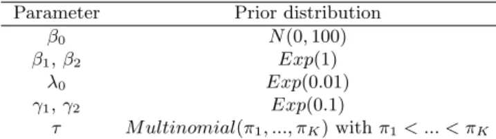
algorithm to explore higher dose levels of agent B and actively learn the shape of the dose-eﬃcacy curve, thereby improving the ODC selection accuracy. In our simulation study, we took π = (0.14, 0.20, 0.28, 0.39), which led to good operating characteristics across various scenarios. A summary of prior distributions is given in Table 1. After specifying the prior distributions, we sampled posterior distributions (2) and (3) using the Gibbs sampler.

We next discuss how to specify the eﬀective doses (i.e., uj’s and vk’s in the toxicity

model, and wj’s and zk’s in the eﬃcacy model) based on the prior estimates of the

single-agent toxicity and efficacy probabilities. In practice, before two single-agents are to be combined, each of them typically has been studied individually. For example, prior to the solid tumor clinical trial that combines imatinib with paclitaxel (Pishvaian et al., 2012), many phase I and II trials have been conducted to study the single-agent toxicity and efficacy profiles for imatinib (Ramanathan et al., 2008; Gibbons et al., 2008; Lipton et al., 2010; van Oosterom et al., 2001) and paclitaxel (Kato et al., 2011; Tsimberidou et al., 2011; Takano et al., 2002; Lim et al., 2010; Horiguchi et al., 2009). Therefore, we often have good prior estimates of the single-agent toxicity and efficacy probabilities for each of the agents. The purpose of defining and using the effective doses is to match the prior estimates of (single-agent) toxicity and efficacy probabilities under our model with those elicited from the prior information. By doing so, we incorporate the available single-agent dose-toxicity and -efficacy information into our model and thus improve the efficiency of the design. This approach has been previously used for dose finding in single-agent trials (Chevret, 2006; Zohar et al., 2013) and drug-combination trials (Liu and Ning, 2013).

(13)

for the jth level of agent A and the kth level of agent B, respectively, and ˆqj0≡ 1 − ˆSj0(T )

and ˆq0k≡ 1 − ˆS0k(T ) denote the estimates of the single-agent eﬃcacy probabilities for the

jth level of agent A and the kth level of agent B (at the end of follow-up). Under toxicity model (1), by setting the dosage of agent B (or A) as zero, we obtain the single-agent toxicity model logit(pj0) = β0+ β1uj for agent A and logit(p0k) = β0+ β2vk for agent B.

Therefore, based on the prior estimates ˆpj0 and ˆp0k , we backsolve the eﬀective doses uj

and vk as

uj = {logit(ˆpj0)− ˆβ0}/ ˆβ1

vk = {logit(ˆp0k)− ˆβ0}/ ˆβ2,

where ˆβ0 and ˆβ1 are prior means of β0 and β1. Similarly, under eﬃcacy survival model

(2), the single-agent eﬃcacy model is Sj0(t) = exp{−λ0.t.exp(γ1wj)} for agent A and

S0k(t) = exp[−λ0.t.exp{γ2(zk1(k < τ) + zτ1(k ≥ τ))}] for agent B. We determine the

eﬀective doses

wj = log[−log{1 − ˆqj0}/(ˆλ0T )]/ˆγ1

zk = log[−log{1 − ˆq0k}/(ˆλ0T )]/ˆγ2,

where ˆλ0, ˆγ1, ˆγ2 are prior estimates of the corresponding parameters, and ˆτ is the highest

dose levels.

3.4. Dose-finding algorithm

At the beginning of the trial, data are very sparse and the estimates of the toxicity and efficacy models are highly unreliable. To improve the reliability of dose finding, we use a start-up phase to collect some preliminary data prior to switching to the formal model-based dose-finding algorithm.

(14)

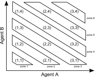
We adopted a start-up phase similar to that proposed by Huang et al. (2007), which divides the dose combination matrix into a sequence of zones along the diagonal from low doses to high doses (see Figure 1), and then conducts a “3+3” type dose escalation across the zones. Specifically, we initiate the start-up phase by treating the first cohort of 3 patients at the lowest zone, i.e., the lowest combination (1, 1), and then continuously escalate the dose to higher dose zones until we first encounter a zone in which all doses are “closed.” Given a dose, if more than 1 patient were to experience toxicity out of the 3 or 6 patients who have been administered that dose, we close the dose and require that all higher doses (i.e., any combination having a higher dose level of A or B or A and B) are automatically closed and not eligible for use in treating future patients in the start-up phase. More precisely, if we close dose combination (j, k), we also close higher doses {(j′, k′); j′ ≥ j and k′ ≥ k}. The “closed” dose combinations can be reopened later to treat patients in the subsequent model-based dose-finding phase if the accumulating data indicate that they are actually safe. The dose escalation across zones is analogous to the traditional “3+3” dose escalation rule: among three patients, if we observe no toxicity, we escalate the dose; if more than 2 patients experience toxicity, we close the dose; and if 1 patient experiences toxicity, we treat three more patients at the current dose. In the latter case, if 0 or 1 out of the 6 patients experiences toxicity, we escalate the dose; otherwise we close the dose. When we escalate to a higher dose zone, if there are multiple combinations that are not closed in that zone, we simultaneously assign patients to each of the combinations.

After the start-up phase, we switch to the model-based dose-finding phase. Let θ and ξ denote the prespecified toxicity upper bound and efficacy lower bound, respectively. Let N denote the total sample size, and n denote the number of patients treated in the trial. We

(15)

deﬁne that a combination (j, k) is admissible if it satisﬁes the safety requirement

P (pjk> θ) < CT (4)

and also the eﬃcacy requirement

P (Sjk(T ) > ξ)≥ CE1(n ≥ N/2), (5)

where CT and CE are the respective probability thresholds for toxicity and eﬃcacy. Note

that the efficacy requirement (5) takes effect when only half of the patients have been enrolled, as controlled by the indicator function 1(n ≥ N/2). We found that introducing the efficacy condition too early caused a high frequency of misclassification of the admissible doses as inadmissible and thus resulted in the early termination of the trial. This situation can arise because, compared to the evaluation of the toxicity condition (4), the reliable evaluation of the efficacy condition (5) requires more data, as the efficacy outcome is not immediately observable and the efficacy model is relatively more complicated.

Let (j, k) denote the current dose, A denote the set of combinations that have been previously used to treat patients, and B = {(j′, k′); j′ ≤ j + 1, k′ ≤ k + 1, and (j′, k′) ̸= (j+1, k+1)} denote the set of combinations for which the doses are not two levels higher than the current dose (j, k). Our model-based dose-finding algorithm can be described as follows: after the start-up phase, we assign the next cohort of patients to the optimal combination that is admissible and which also has the highest estimate of efficacy, i.e., 1− ˆS(T ), selected from the setA ∪ B. If several such optimal combinations exist, e.g., the efficacy has reached a plateau with respect to the dose level of the MTA, we select the one with the lowest toxicity probability (e.g., the optimal combination with the lowest MTA dose level) to treat the new cohort. At any time, if all combinations are not admissible, then we terminate the trial; otherwise, we continue this dose assignment process until the maximum sample size

(16)

is reached. At the end of the trial, we select the ODC as the admissible combination that has the highest estimate of eﬃcacy along with the lowest estimate of toxicity.

4. Numerical Studies 4.1. Simulation study

We carried out extensive simulations to evaluate the operating characteristics of the pro-posed phase I/II design. Taking the setting of the aforementioned solid tumor trial, we assumed 3 dose levels for cytotoxic agent A (i.e., paclitaxel) and 4 dose levels for molec-ularly targeted agent B (i.e., imatinib), resulting in a total of 12 combinations. We took the initial guesses of the single-agent toxicity and efficacy as (0.2, 0.3, 0.4) and (0.3, 0.4, 0.5), respectively, for agent A, and (0.12, 0.2, 0.3, 0.4) and (0.3, 0.4, 0.5, 0.59) for agent B. The maximum sample size was 75 and patients were treated sequentially in cohorts of size 3. We assumed that the patient accrual followed a Poisson process with the rate of 1/3.5 patients per week. The toxicity upper bound was θ = 0.30 and the efficacy lower bound was ξ = 0.20. We set the toxicity threshold as CT = 0.85 and the efficacy threshold as

CE = 0.10, and took the prior probabilities of the dose-eﬃcacy curve reaching a plateau

at the different dose levels of agent B as (0.16, 0.21, 0.27, 0.36). We considered 8 different dose-toxicity and efficacy scenarios (see Table 2), representing what we may encounter in practice. We assumed that toxicity was quickly evaluable, while the evaluation of efficacy required 7 weeks, i.e., T = 7 weeks. Under each scenario, we assumed that at each com-bination, the time to efficacy followed an exponential distribution. The parameter of the exponential distribution was chosen such that at the end of follow-up, the efficacy rate of each dose combination (i.e., 1−Sjk(T )) matched those displayed in Table 2. As a result, the

parameter of the exponential distribution had to vary across doses. Under each scenario, we conducted 1,000 simulations.

(17)

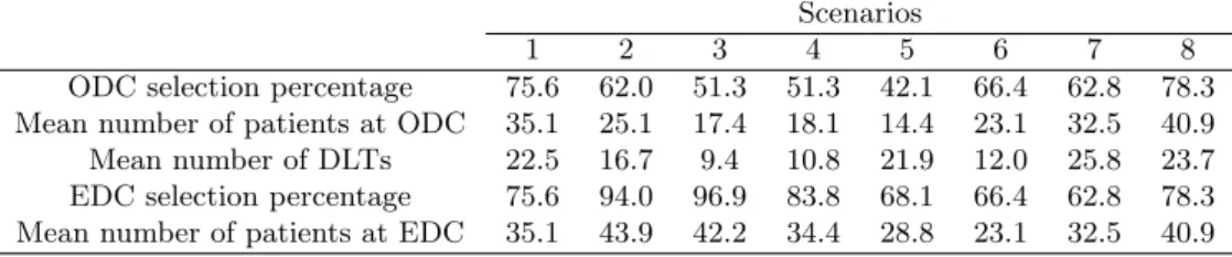
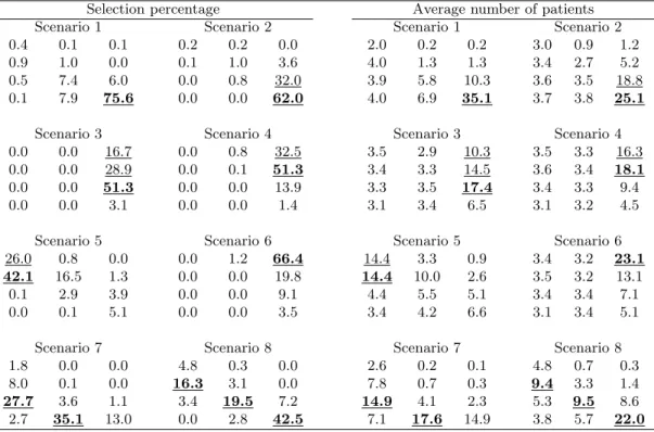
Table 3 shows the simulation results, including the ODC selection percentage, the av-erage number of patients assigned to the ODC, and the avav-erage number of dose-limiting toxicities (DLTs). We also reported the “effective dose combination” (EDC) selection per-centage, defining the EDCs as the admissible combinations that yield the same (highest) efficacy as the ODC and which also have acceptable toxicity, i.e., the toxicity probability of the EDC is not necessarily the lowest among several equally efficacious combinations. For example, in scenario 2 in Table 2, both (3, 1) and (3, 2) have the same high efficacy rate of 55% and acceptable toxicity rates not higher than 30%. The ODC is (3, 1) as it has a lower toxicity probability or lower MTA dose level (i.e., agent B); whereas both (3, 1) and (3, 2) are EDCs as they are both safe and efficacious. Although the ODC is optimal, in practice, the EDCs are also of interest due to their high efficacy even though their dose of agent B may be higher than what is actually needed. Note that under our definitions, the ODC is one of the EDCs, but not vice versa. Table 4 provides more detailed simulation results for the selection percentages and the number of patients treated at each dose combination.

In general, the proposed design performed well across 8 scenarios. The ODC and EDC selection percentages were generally greater than 50%, and the design allocated a large number of patients to the ODC and EDCs. Specifically, in scenario 1, the dose-efficacy curve (approximately) plateaus at the lowest dose level of the targeted agent B, and the ODC is the combination (3, 1), which yields the highest efficacy with the lowest dose of the targeted agent. This ODC is also the only EDC in scenario 1. To mimic what may happen in practice, we designed the scenarios to allow for some variation in efficacy, even when it has reached the plateau. The proposed design selected the ODC 75.6% of the time, and allocated on average 35.1 patients to the ODC. As in scenario 1, in scenario 2, the dose-efficacy curve plateaued from the lowest dose level of the targeted agent B with (3, 1)

(18)

as the ODC, but with two EDCs, i.e., (3, 1) and (3, 2). Note that combinations (3, 3) and (3, 4) have high efficacy probabilities that are similar to that of the ODC (3, 1), but they are not EDCs because they are not admissible combinations due to high toxicity. In this case, the proposed design selected the ODC and EDCs 62.0% and 94.0% of the time. In scenario 3, the dose-efficacy curve plateaus after dose level 1 of agent B. The ODC and EDC selection percentages in that scenario were 51.3% and 96.9%, respectively. Scenarios 4 and 5 both have efficacy plateaus after dose level 2 of agent B, but with different locations for the ODC and EDCs. In these two cases, the ODC selection percentages were more than 40%. Scenarios 6 to 8 simulate efficacy monotonically increasing with the dose of agent B (e.g., agent B does not reach a level of saturation within the range of the investigational doses), with different numbers for the ODCs, which is similar to what may happen in conventional combination trials with two cytotoxic agents. The simulations demonstrate that our proposed design performed well and achieved ODC and EDC selection percentages that were all higher than 60%, suggesting that the proposed design can also be applied to the combination of two cytotoxic agents.

4.2. Sensitivity analysis

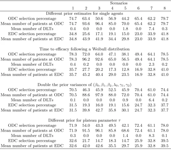
We performed sensitivity analyses to study the robustness of our design. We varied four fac-tors: (1) the prior estimates of the single-agent toxicity and eﬃcacy probabilities; (2) the dis-tribution of time to eﬃcacy; (3) the variance of the prior disdis-tribution for β0, β1, β2, λ0, γ1, andγ2;

and (4) the prior distribution for τ . We assumed that the single-agent toxicity and ef-ficacy probabilities, used to determine the “effective” dose in the toxicity and efficacy model, were (0.06, 0.12, 0.2) and (0.12, 0.2, 0.3) for agent A, and (0.06, 0.12, 0.2, 0.3) and (0.4, 0.5, 0.59, 0.67) for agent B. We simulated the time to efficacy from a Weibull tion with a fixed shape parameter of 3. We chose the scale parameter of the Weibull

(19)

distribu-tion such that the eﬃcacy probabilities at the end of follow-up, i.e., 1−S(T ), matched those given in Table 2. We inﬂated the prior variances of parameters β0, β1, β2, λ0, γ1, and γ2 by

2-fold, and used π = (0.11, 0.17, 0.28, 0.44) as the prior probabilities of τ . Table 5 shows the results of the sensitivity analyses. We can see that the ODC and EDC selection per-centages and the number of patients treated at the ODC and EDCs are generally similar to those reported in Table 3, which suggests that the proposed design is not sensitive to the aforementioned design factors.

4.3. Application

We retrospectively applied our design to the solid tumor trial. As described previously, the trial selectively studied six dose combinations out of 12 possible combinations. Because the dosing schedule used in the original protocol resulted in too many toxicities, the protocol was amended to use a less intensive dose schedule. As a result, ﬁve dose combinations were actually used for dose ﬁnding under the amended schedule, as shown in Table 6. The window for assessing treatment response was set at T = 13 weeks. The trial did not report the time to response; thus, we assumed that it was uniformly distributed within the assessment window. To be consistent with the “3+3” method used by the trial, we set CT= 0.33 and

CE= 0.0, and forbade skipping untried doses during the dose escalation.

The trial started by treating the ﬁrst cohort of 3 patients at the lowest dose combination (60, 400), at which one response and no dose-limiting toxicity (DLT) was observed. Based on the data, our method identiﬁed dose combination (100, 600) as the ODC, with an estimated response rate of 0.54, and thus recommended dose escalation to (80, 400) for treating the second cohort of patients. Among the three patients treated at (80, 400), two responded to the treatment and no DLT was observed. In light of this new information,

(20)

our method estimated combination (100, 600) as the ODC, with an estimated response rate of 0.56. Accordingly, we escalated the dose to (80, 600) for treating the third cohort of 3 patients, among which 2 patients responded to the treatment and no DLT was observed. Our method then escalated the dose and assigned the fourth cohort to dose combination (100, 600), at which we observed 2 responses and no DLT. At that moment, the estimated ODC was dose combination (100, 600), with the estimated response rate of 0.45. Based on this result, our method would retain the current dose and assign the remaining 6 patients to (100, 600); whereas the “3+3” design dictated a dose escalation to (100, 800). At the end of the trial, our design selected (100, 600) as the ODC, while the “3+3” design picked (100, 800). According to the literature, a dose of 600mg of imatinib reaches the plateau of the dose-response curve and actually is the dosage that has been widely administered to cancer patients in practice. It seems that our design successfully identiﬁed that, while the “3+3” design might have resulted in overdosing of patients by selecting a dose of 800mg. 5. Conclusions

We have proposed a Bayesian phase I/II design for trials that combine a cytotoxic agent with a molecularly targeted agent. We assumed that toxicity is quickly evaluable and used a logistic regression model to evaluate toxicity as a binary outcome. In contrast, we assumed that efficacy takes a relatively long time to evaluate, and correspondingly used a proportional hazard model to evaluate efficacy as a time-to-event outcome. To account for the characteristic dose-efficacy curve for MTAs, which initially increases and then plateaus, we incorporated a plateau point into the time-to-efficacy model. During the trial conduct, we continuously updated the model estimates and used them to assign patients to the ODC. We evaluated our design through a simulation study under various practical scenarios. Our design performed well by selecting the optimal dose combination a high percentage of the

(21)

time.

The proposed design assumes that the treatment response can be observed anytime during the followup period. For some clinical trials, the response however can only be ascertained at the end of followup, for example, when the response is deﬁned as a certain percentage of tumor shrinkage at time T . In these cases, rather than modeling the time to response, we can model the time to disease progression (i.e., time to nonresponse), which typically is observable in real time based on patient’s symptoms. The proposed model and design can still be used. We just need to treat t as the time to nonresponse, and accordingly estimate the response rate qjk at T by Sjk(T ), rather than 1− Sjk(T ).

There are several possible extensions of the proposed design to further improve its per-formance or flexibility in order to accommodate different clinical applications. For example, rather than modeling toxicity as a binary outcome, we can use measurements of the various grades of toxicity and model it as an ordinary outcome. This approach uses more refined information and can potentially improve the efficiency of the trial design. In addition, when late-onset toxicity is of concern, we can model toxicity as a time-to-event outcome, as we have done for efficacy. Lastly, our dose assignment and selection criteria focus on efficacy while controlling for toxicity. In some applications, it may be more appropriate to consider the tradeoff between toxicity and efficacy. To accommodate these cases, we can define a utility function for the tradeoff between toxicity and efficacy and then use the utility as the criterion for dose assignment and selection.

Acknowledgements

This work was partially funded by grants from the ANRT (Association Nationale de la Recherche et de la Technologie), “Laboratoires Servier” (CIFRE number 2011/0900), and

(22)

Denis Diderot University-Paris 7 (“Aide `a la mobilit´e internationale 2012”). Yuan’s research was partially supported by Award Number R01 CA154591 and P50 CA098258 from the National Cancer Institute.

(23)

References

Braun, T. M. and S. Wang (2010, Sep). A hierarchical Bayesian design for phase I trials of novel combinations of cancer therapeutic agents. Biometrics 66 (3), 805–812.

Cai, C., Y. Y. and Y. Ji (2014, Jan). A bayesian phase i/ii design for oncology clinical trials of combining biological agents. Journal of the Royal Statistical Society: Series C 63, 159–173.

Chevret, S. (1993, Jun). The continual reassessment method in cancer phase I clinical trials: a simulation study. Stat Med 12 (12), 1093–1108.

Chevret, S. (2006, May). Statistical Methods for dose-Finding Experiments. Statistics in Practice. Chichester: John Wiley and Sons Ltd.

Conaway, M. R., S. Dunbar, and S. D. Peddada (2004, Sep). Designs for single- or multiple-agent phase I trials. Biometrics 60, 661–669.

Druker, B. J. (2002, Feb). Perspectives on the development of a molecularly targeted agent. Cancer Cell 1 (1), 31–36.

Gafter-Gvili, A., A. Leader, R. Gurion, L. Vidal, R. Ram, A. Shacham-Abulaﬁa, I. Ben-Bassat, M. Lishner, O. Shpilberg, and P. Raanani (2011, Aug). High-dose imatinib for newly diagnosed chronic phase chronic myeloid leukemia patients–systematic review and meta-analysis. Am. J. Hematol. 86 (8), 657–662.

Gibbons, J., M. J. Egorin, R. K. Ramanathan, P. Fu, D. L. Mulkerin, S. Shibata, C. H. Takimoto, S. Mani, P. A. LoRusso, J. L. Grem, A. Pavlick, H. J. Lenz, S. M. Flick, S. Reynolds, T. F. Lagattuta, R. A. Parise, Y. Wang, A. J. Murgo, S. P. Ivy, and S. C. Remick (2008, Feb). Phase I and pharmacokinetic study of imatinib mesylate in patients

(24)

with advanced malignancies and varying degrees of renal dysfunction: a study by the National Cancer Institute Organ Dysfunction Working Group. J. Clin. Oncol. 26 (4), 570–576.

Hoering, A., M. LeBlanc, and J. Crowley (2011, Feb). Seamless phase I-II trial design for assessing toxicity and eﬃcacy for targeted agents. Clin. Cancer Res. 17 (4), 640–646.

Horiguchi, J., Y. Rai, K. Tamura, T. Taki, K. Hisamatsu, Y. Ito, T. Seriu, and T. Tajima (2009, Feb). Phase II study of weekly paclitaxel for advanced or metastatic breast cancer in Japan. Anticancer Res. 29 (2), 625–630.

Huang, X., S. Biswas, Y. Oki, J. P. Issa, and D. A. Berry (2007, Jun). A parallel phase I/II clinical trial design for combination therapies. Biometrics 63 (2), 429–436.

Kato, K., M. Tahara, S. Hironaka, K. Muro, H. Takiuchi, Y. Hamamoto, H. Imamoto, N. Amano, and T. Seriu (2011, Jun). A phase II study of paclitaxel by weekly 1-h infusion for advanced or recurrent esophageal cancer in patients who had previously received platinum-based chemotherapy. Cancer Chemother. Pharmacol. 67 (6), 1265– 1272.

Le Tourneau, C., V. Dieras, P. Tresca, W. Cacheux, and X. Paoletti (2010, Mar). Current challenges for the early clinical development of anticancer drugs in the era of molecularly targeted agents. Target Oncol 5 (1), 65–72.

Le Tourneau, C., H. K. Gan, A. R. Razak, and X. Paoletti (2012, Dec). Eﬃciency of new dose escalation designs in dose-ﬁnding phase I trials of molecularly targeted agents. PLoS ONE 7 (12), e51039.

(25)

(2011, Jul). Heterogeneity in the deﬁnition of dose-limiting toxicity in phase I cancer clinical trials of molecularly targeted agents: a review of the literature. Eur. J. Can-cer 47 (10), 1468–1475.

Lim, W. T., E. H. Tan, C. K. Toh, S. W. Hee, S. S. Leong, P. C. Ang, N. S. Wong, and B. Chowbay (2010, Feb). Phase I pharmacokinetic study of a weekly liposomal paclitaxel formulation (Genexol-PM) in patients with solid tumors. Ann. Oncol. 21 (2), 382–388.

Lipton, A., C. Campbell-Baird, H. Harvey, C. Kim, L. Demers, and L. Costa (2010, Feb). Phase I trial of zoledronic acid + imatinib mesylate (Gleevec) in patients with bone metastases. Am. J. Clin. Oncol. 33 (1), 75–78.

Liu, S. and J. Ning (2013, Sep). A bayesian dose-ﬁnding design for drug combination trials with delayed toxicities. Bayesian Analysis 8 (3), 703–722.

Mandrekar, S. J., Y. Cui, and D. J. Sargent (2007, May). An adaptive phase I design for identifying a biologically optimal dose for dual agent drug combinations. Stat Med 26, 2317–2330.

O’Quigley, J. and X. Paoletti (2003, Jun). Continual reassessment method for ordered groups. Biometrics 59 (2), 430–440.

Pishvaian, M. J., R. Slack, E. Y. Koh, J. H. Beumer, M. L. Hartley, I. Cotarla, J. Deeken, A. R. He, J. Hwang, S. Malik, K. Firozvi, M. Liu, B. Elston, S. Strychor, M. J. Egorin, and J. L. Marshall (2012, Dec). A Phase I clinical trial of the combination of imatinib and paclitaxel in patients with advanced or metastatic solid tumors refractory to standard therapy. Cancer Chemother. Pharmacol. 70 (6), 843–853.

(26)

J. De-Bono, I. Judson, and S. Kaye (2009, May). Clinical beneﬁt in Phase-I trials of novel molecularly targeted agents: does dose matter? Br. J. Cancer 100 (9), 1373–1378.

Ramanathan, R. K., M. J. Egorin, C. H. Takimoto, S. C. Remick, J. H. Doroshow, P. A. LoRusso, D. L. Mulkerin, J. L. Grem, A. Hamilton, A. J. Murgo, D. M. Potter, C. P. Belani, M. J. Hayes, B. Peng, and S. P. Ivy (2008, Feb). Phase I and pharmacokinetic study of imatinib mesylate in patients with advanced malignancies and varying degrees of liver dysfunction: a study by the National Cancer Institute Organ Dysfunction Working Group. J. Clin. Oncol. 26 (4), 563–569.

Takano, M., Y. Kikuchi, T. Kita, M. Suzuki, M. Ohwada, T. Yamamoto, K. Yamamoto, H. Inoue, and K. Shimizu (2002, May-Jun). Phase I and pharmacological study of single paclitaxel administered weekly for heavily pre-treated patients with epithelial ovarian cancer. Anticancer Res. 22 (3), 1833–1838.

Thall, P. F., R. E. Millikan, P. Mueller, and S. J. Lee (2003, Sep). Dose-ﬁnding with two agents in Phase I oncology trials. Biometrics 59 (3), 487–496.

Tsimberidou, A. M., K. Letourneau, S. Fu, D. Hong, A. Naing, J. Wheler, C. Uehara, S. E. McRae, S. Wen, and R. Kurzrock (2011, Jul). Phase I clinical trial of hepatic arterial infusion of paclitaxel in patients with advanced cancer and dominant liver involvement. Cancer Chemother. Pharmacol. 68 (1), 247–253.

van Oosterom, A. T., I. Judson, J. Verweij, S. Stroobants, E. Donato di Paola, S. Dimitri-jevic, M. Martens, A. Webb, R. Sciot, M. Van Glabbeke, S. Silberman, and O. S. Nielsen (2001, Oct). Safety and eﬃcacy of imatinib (STI571) in metastatic gastrointestinal stro-mal tumours: a phase I study. Lancet 358 (9291), 1421–1423.

(27)

Wages, N. A., M. R. Conaway, and J. O’Quigley (2011, Dec). Continual Reassessment Method for Partial Ordering. Biometrics.

Yin, G. and Y. Yuan (2009, May). Bayesian dose ﬁnding in oncology for drug combinations by copula regression. JRSS 58, 211–224.

Yuan, Y. and G. Yin (2008, Nov). Sequential continual reassessment method for two-dimensional dose ﬁnding. Stat Med 27 (27), 5664–5678.

Yuan, Y. and G. Yin (2011, Jan). Bayesian Phase I/II Adaptively Randomized Oncology Trials With Combined Drugs. Ann Appl Stat 5 (2A), 924–942.

Zohar, S., M. Resche-Rigon, and S. Chevret (2013, Jun). Using the continual reassessment method to estimate the minimum eﬀective dose in phase II dose-ﬁnding studies: a case study. Clin Trials 10 (3), 414–421.

(28)

Table 1. Prior distributions for model parameters.

Parameter Prior distribution

β0 N (0, 100)

β1, β2 Exp(1)

λ0 Exp(0.01)

γ1, γ2 Exp(0.1)

(29)

Table 2. Eight toxicity and efficacy scenarios for the combination of a cytotoxic agent (agent A) with a molecularly targeted agent (agent B). The optimal dose combinations (ODCs) are in bold and the effective dose combinations (EDCs) are underlined. The dashed lines indicate the dose level of the MTA at which the efficacy plateaus.

Agent A Agent A

Agent 1 2 3 1 2 3 1 2 3 1 2 3

B Toxicity Eﬃcacy Toxicity Eﬃcacy

Scenario 1 Scenario 2 4 0.45 0.50 0.65 0.27 0.42 0.56 0.30 0.45 0.55 0.28 0.43 0.57 3 0.30 0.45 0.55 0.26 0.41 0.56 0.15 0.30 0.45 0.27 0.42 0.56 2 0.15 0.30 0.45 0.25 0.41 0.55 0.12 0.15 0.30 0.26 0.40 0.55 1 0.10 0.15 0.30 0.25 0.40 0.55 0.08 0.10 0.15 0.25 0.40 0.55 Scenario 3 Scenario 4 4 0.10 0.15 0.30 0.37 0.52 0.67 0.10 0.15 0.30 0.32 0.46 0.61 3 0.07 0.10 0.15 0.36 0.51 0.66 0.08 0.10 0.15 0.30 0.45 0.60 2 0.05 0.08 0.10 0.35 0.50 0.65 0.04 0.05 0.10 0.20 0.30 0.40 1 0.01 0.05 0.07 0.15 0.25 0.35 0.01 0.03 0.07 0.05 0.10 0.20 Scenario 5 Scenario 6 4 0.30 0.55 0.65 0.41 0.56 0.67 0.10 0.15 0.30 0.40 0.55 0.70 3 0.15 0.45 0.55 0.40 0.55 0.65 0.07 0.10 0.15 0.25 0.40 0.55 2 0.10 0.30 0.45 0.15 0.20 0.25 0.05 0.08 0.10 0.15 0.30 0.40 1 0.05 0.15 0.30 0.05 0.10 0.15 0.01 0.05 0.07 0.05 0.10 0.30 Scenario 7 Scenario 8 4 0.50 0.60 0.65 0.50 0.60 0.70 0.45 0.55 0.65 0.50 0.60 0.70 3 0.45 0.55 0.60 0.45 0.50 0.60 0.30 0.45 0.60 0.45 0.52 0.63 2 0.30 0.45 0.50 0.30 0.45 0.50 0.15 0.30 0.50 0.30 0.45 0.50 1 0.15 0.30 0.45 0.15 0.30 0.45 0.10 0.15 0.30 0.20 0.30 0.45

(30)

Table 3. Selection percentage of the optimal dose combination (ODC) and effective dose combination (EDC), the average number of patients treated at the ODC and EDC, and the average number of dose-limiting toxicities (DLTs).

Scenarios

1 2 3 4 5 6 7 8

ODC selection percentage 75.6 62.0 51.3 51.3 42.1 66.4 62.8 78.3 Mean number of patients at ODC 35.1 25.1 17.4 18.1 14.4 23.1 32.5 40.9 Mean number of DLTs 22.5 16.7 9.4 10.8 21.9 12.0 25.8 23.7 EDC selection percentage 75.6 94.0 96.9 83.8 68.1 66.4 62.8 78.3 Mean number of patients at EDC 35.1 43.9 42.2 34.4 28.8 23.1 32.5 40.9

(31)

Table 4. ODC (in boldface) and EDC (underlined) selection percentages and the average number of patients treated at each combination.

Selection percentage Average number of patients

Scenario 1 Scenario 2 Scenario 1 Scenario 2

0.4 0.1 0.1 0.2 0.2 0.0 2.0 0.2 0.2 3.0 0.9 1.2

0.9 1.0 0.0 0.1 1.0 3.6 4.0 1.3 1.3 3.4 2.7 5.2

0.5 7.4 6.0 0.0 0.8 32.0 3.9 5.8 10.3 3.6 3.5 18.8

0.1 7.9 75.6 0.0 0.0 62.0 4.0 6.9 35.1 3.7 3.8 25.1

0.0 0.0 16.7 0.0 0.8 32.5 3.5 2.9 10.3 3.5 3.3 16.3

0.0 0.0 28.9 0.0 0.1 51.3 3.4 3.3 14.5 3.6 3.4 18.1

0.0 0.0 51.3 0.0 0.0 13.9 3.3 3.5 17.4 3.4 3.3 9.4

0.0 0.0 3.1 0.0 0.0 1.4 3.1 3.4 6.5 3.1 3.2 4.5

26.0 0.8 0.0 0.0 1.2 66.4 14.4 3.3 0.9 3.4 3.2 23.1

42.1 16.5 1.3 0.0 0.0 19.8 14.4 10.0 2.6 3.5 3.2 13.1

0.1 2.9 3.9 0.0 0.0 9.1 4.4 5.5 5.1 3.4 3.4 7.1

0.0 0.1 5.1 0.0 0.0 3.5 3.4 4.2 6.6 3.1 3.4 5.1

1.8 0.0 0.0 4.8 0.3 0.0 2.6 0.2 0.1 4.8 0.7 0.3

8.0 0.1 0.0 16.3 3.1 0.0 7.8 0.7 0.3 9.4 3.3 1.4

27.7 3.6 1.1 3.4 19.5 7.2 14.9 4.1 2.3 5.3 9.5 8.6

(32)

Table 5. Results of the sensitivity analysis.

Scenarios

1 2 3 4 5 6 7 8

Diﬀerent prior estimates for single agents

ODC selection percentage 74.7 63.4 50.6 56.9 44.2 65.4 62.2 79.7 Mean number of patients at ODC 74.7 93.6 96.4 85.0 70.0 65.4 62.2 79.7

Mean number of DLTs 0.4 0.0 0.0 0.0 1.8 0.0 7.4 0.3

EDC selection percentage 34.8 25.6 17.1 19.1 15.0 23.0 33.9 41.8 Mean number of patients at EDC 34.8 43.9 41.9 34.4 29.8 23.0 33.9 41.8

Time to eﬃcacy following a Weibull distribution

Double the prior variances of (β0, β1, β2, λ0, γ1, γ2)

Diﬀerent prior for plateau parameter τ

(33)

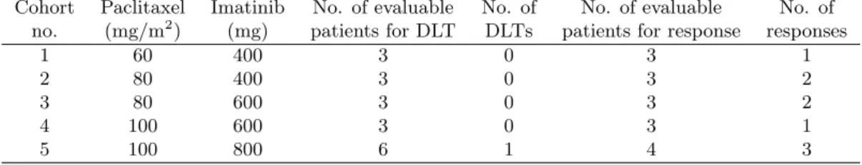
Table 6. Summarized data from the case study combination clinical trial involving Imatinib with Pacli-taxel. The number of responses is the addition of stabilities and partial responses.

Cohort Paclitaxel Imatinib No. of evaluable No. of No. of evaluable No. of no. (mg/m2) (mg) patients for DLT DLTs patients for response responses

1 60 400 3 0 3 1

2 80 400 3 0 3 2

3 80 600 3 0 3 2

4 100 600 3 0 3 1

(34)

Figure 1. An illustration of combination zones for the start-up phase. (1,3) (2,3) (3,4) (3,3) (1,2) (2,2) (3,2) (2,4) (1,1) (2,1) (1,4) (3,1) Agent A A ge nt B

zone 1 zone 2 zone 3

zone 4 zone 5 zone 6