Faculté des Sciences Economiques Avenue du 1er-Mars 26 CH-2000 Neuchâtel www.unine.ch/seco
PhD Thesis submitted to the Faculty of Economics and Business Institute of Financial Analysis
University of Neuchâtel
For the degree of PhD in Finance by
Ali MARAMI
Accepted by the dissertation committee:
Prof. Michel Dubois, University of Neuchâtel, thesis director Prof. Rüdiger Fahlenbrach, EPFL
Prof. Peter Fiechter, University of Neuchâtel Prof. Jérôme Taillard, Boston College, USA
Prof. Philip Valta, HEC Paris, France
Defended on 27 August 2014
Acknowledgments
First of all, I would express my gratitude to my advisor Professor Michel Dubois for guiding me during the entire PhD research. I appreciate his inspiration, encouragement and support through these valuable years at the University of Neuchatel. I would also like to thank Rüdiger Fahlenbrach, Peter Fiechter, Jérôme Taillard and Philip Valta who have accepted to be part of my dissertation committee. I am certain that their comments enrich my research at the different stages of this thesis.
My further gratitude goes to Jean Noël Barrot, Stefano Puddu, Ehraz Refayet, Carolina Salva, Tobias Scheinert, and seminar participants at the World Finance Conference, the FMA Europe 2013, and the AFFI International Conference in Paris 2013 for their valuable comments and suggestions. I am also grateful to all my Ph.D. student colleagues as well as participants of finance seminars at University of Neuchâtel for their significant impact on my research through discussions and comments.
This thesis is impossible without the encouragement and support of my family. I am indebted to them.
Summary:
In this dissertation, I analyze the proxies used in literature as the determinants of firm value to identify the core variables in modeling firm value. Using these variables, I evaluate the impact of interest rate derivatives on firm value. More specifically, I find that interest rate derivatives imposed in credit agreements has a positive impact on firm value in contrast to those used voluntarily for which the motive behind the use of derivatives is not clear for equity holders. The impact of systematic risk in placement structure of debt is also studied. I show that the impact of systematic risk on cost of debt is higher for public debts compared to those for private credit agreements. However, the emergence of loan secondary market diminishes this difference.
Keywords:
Firm value; interest rate; risk management; derivatives; hedging; agency conflicts; systematic risk; public debt; private debt; loan secondary market.
Table of Contents
Introduction ... 1
Chapter 1: Which factors are important in firm valuation? ... 4
1.1 Introduction ... 4
1.2 The determinants of firm value ... 8
1.3 Empirical Analysis ... 14
1.4 Specification and power of the regression model ... 20
1.5 Conclusion ... 26
References ... 27
Appendix ... 34
Chapter 2: Which Firms Benefit from Interest Rate Hedging? ... 58
2.1 Introduction ... 58
2.2 Data and methodology ... 65
2.3 IRP and firm value... 68
2.4 Firm value, IRP, and alternative monitoring tools ... 74
2.5 Information asymmetries, mandatory hedging and firm value ... 79
2.6 Conclusion ... 86
References ... 88
Appendix ... 93
Chapter 3: Why do firms with investment grade rating borrow from private lenders? 103 3.1 Introduction ... 103
3.2 Review of the literature ... 107
3.3 Data and methodology ... 111
3.4 Empirical tests and results ... 114
3.5 Selection biases and simultaneity ... 119
3.6 Conclusion ... 125
References ... 126
1
Introduction
In this dissertation, I focus on the determinants of firm value. More specifically, I start by investigating the main determinants and core factors in modelling the “normal” value of the firm. I review papers published in major accounting, economic and finance journals that relate firm value to a set of determinants. Consistent with existing theories, this review reveals that profitability, risk, growth, payout policies and size are the main determinants of firm value. However, the proxies used for each factor is extremely diverse. Therefore, I apply Bayesian Information Criterion (BIC) to find variables with highest explanatory power. This analysis identifies six core variables for firm value. I also test the specification and power of the model based on these core variables by conducting a pseudo Mont Carlo simulation. The outcome of this research provides an in-depth understating of determinants of firm value as well as a baseline model to be applied in my research on the impact of risk management on firm value.
In chapter two, I study the interplay between the use of financial derivatives and firm value. I leverage my findings in my research on firm value and analyze the impact of the interest rate derivatives on firm value. Market frictions such as income tax, bankruptcy costs and access to the financial markets bolster potentials for value generation by risk management. For instance, risk management reduces the volatility of cash flows. As a result, it reduces the present value of tax liabilities when the tax function is convex and diminishes the probability of bankruptcy in unfavorable states of economy. Financial derivatives are one of the prevailing tools in risk management. International Swap and Derivative Association and Bank of International Settlement (BIS) frequently report a significant increase in the use of derivatives. For instance, according to BIS report, the notional value of interest rate derivatives increased from $3.3 trillion in 2000 to more than $35.6 trillion in 2009. However, these financial derivatives could be used for other purposes rather than risk management.
2
Stulz (1984) and Smith and Stulz (1985) argue that managers may hold derivative positions for their own advantage that might not be aligned with shareholders’ interests. Consistent with this idea, there is evidence that some firms use financial instruments for speculation; see e.g., Faulkender (2005) and Géczy, Minton, and Schrand (2007). This agency conflict accounts for inconclusive result of researches on unconditional use of derivatives and firm value. Therefore, I turn my attention on the use of derivatives imposed by creditors on firm value. More specifically, I investigate the impact of interest rate protection covenants (IRPC) in syndicated loans on firm value. An IRPC clarifies the use of derivatives to both shareholders and bondholders for the purpose of risk management. Consequently, it alleviates the uncertainty in the motive behind the use of derivatives.
Using a panel of US firms exposed to interest rate risk between 1998 and 2007, I show that mandatory interest rate hedging has an economically large and statistically significant positive impact on firm value. This finding is robust to various competing hypotheses including the existence of additional covenants enhancing firm value, stricter corporate governance rules, and more intensive competition on the product market. To check the robustness of this result to a potential selection bias, I use a propensity score matching and my results are not altered. To reduce endogeneity concerns, I use the introduction of FAS133 rule as a natural experiment. This accounting rule imposes the disclosure of hedging policies, which reduces the ambiguity about interest rate derivatives usage. I find that, after the implementation of the rule, interest rate hedging has a positive impact on firm value. Finally, this analysis shows that this value is created by the relaxation of the financial constraint that allows a higher level of investment and, to a less extent, the reduction of cost of debt.
The outcome of this chapter motivates me to study the interplay between firm risk and debt structure. In fact, working on firms issued syndicated loans, I notice that a large portion of firms with investment grade rating finance their projects through private placement. The
3
literature on the placement structure of debt posits information asymmetries as the main determinants of debt structure. In other word, private lenders are superior to public creditors in financing “information-problematic” firms (Carey, Post and Sharpe, 1998). However, information asymmetry is not an incentive for firms with investment grade rating. Several studies document the impact of systematic risks similar to those in equity price on cost of debt, e.g. Elton, Gruber, Agrawal, and Mann (2001). Since private creditors have a different investment horizon from that of public bond holders, I conjecture that private lenders have a distinct expectation for price of systematic risk compare to public lenders. As a result, in chapter three, I study the systematic risk of private and public borrowers in two groups of investment and speculative credit ratings. I also analyze the impact of emerging secondary loan market on the difference between systematic risk of public and private lenders.
To conclude, the results of my research on firm value complement the literature that examines the determinants of firm value. While most of the previous research considers the main determinants as control variables, I suggest which proxies really matter. I also provide novel empirical evidence of the impact of interest rate derivatives usage on firm value by comparing non-users, voluntary and mandatory users. It is also a step forward to an unbiased estimation of the influence of derivatives on firm value by focusing on derivatives usage imposed by creditors rather than that decided by managers alone. Last but not least, this research opens a new chapter in the debt structure literature by contrasting the price of systematic risk in private and public debt market. I also show that how secondary market diminishes the advantage of private lending in information asymmetry and controlling incentives.
4
Chapter 1: Which factors are important in firm valuation?
(In collaboration with Michel Dubois)1.1 Introduction
Variables affecting firm value are of major interest for both corporate finance and asset pricing. A significant change in these variables, at a given point in time, allows the quantification of their real impact on firm value. Frequently, this identification consists of two steps: (a) the computation of cumulated abnormal stock returns around the event date (event studies) and (b) the estimation of a regression with cumulated abnormal returns as the dependent variable, the independent variables being the variable of interest and a set of controls that determine firm value. However, this identification strategy is feasible when the date and the magnitude of the change in the variable of interest are observable with a reasonable degree of accuracy; see, e.g., Kothari and Warner (2008). It also assumes that the event is not partially anticipated, which smooth the market reaction, and that wealth transfers between stockholders and creditors are absent. An alternative strategy consists in regressing Tobin’s Q, a proxy for firm value, against the variable of interest1 and a set of contemporaneous firm value determinants measured at
equally spaced intervals. The former strategy has been employed routinely in finance and more generally, in economics, while the latter has been used more recently. It is popular for studying the impact of corporate governance, the structure of the board and specific manager’s actions like the impact of derivatives usage, cash holding, corporate diversification and foreign listing.
In this paper, we study which variables are the core factors in firm valuation, whether the corresponding model is well specified and has power to detect changes in firm value when a specific variable of interest is added to the baseline model. We first identify the variables used in the literature. While there is a large consensus on the role of profitability, risk, growth, the
5
payout policy and size as the main determinants of firm value, the proxies for these factors are extremely diverse. We examine which proxies explain firm value and, more importantly, exhibit a reliable sign. For that purpose, we follow a procedure similar to Frank and Goyal (2009). We collect the proxies of the core factors and select our baseline model with the Bayesian Information Criterion (BIC). This approach should help reduce the diversity of the control variables. Secondly, we evaluate the performance of this baseline model. Beyond the core factors, we aim at testing whether the model is well specified and has power to detect a variable of interest not already incorporated in the model. We explore these properties through pseudo Monte Carlo simulations.
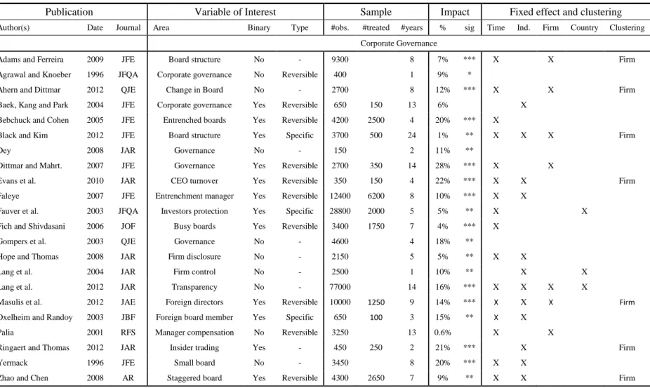
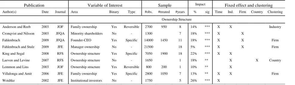
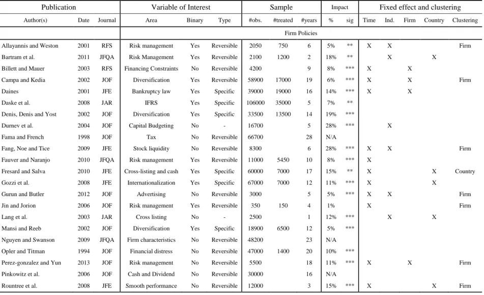
We begin by reviewing papers published in major accounting, economic and finance journals that relate firm value to a set of determinants. We select empirical papers, published between 1995 and 20132, containing the following key words in the text: “Q ratio”, “Tobin’s Q”, “firm
value”, “firm valuation” and “firm performance”. Then, we retain exclusively those papers where Tobin’s Q is the dependent variable. In total, we find fifty-two papers that match our requirements (fourty in finance journals, ten in accounting journals and two in economic journals). More specifically, their focus is on corporate governance (twenty-two papers), ownership structure (nine papers), followed by risk management (five papers), diversification, cross-listing and other corporate policies (sixteen papers).
These empirical papers typically study whether a variable of interest affects Tobin’s Q after controlling for its main contemporaneous determinants (forty-nine papers). However, the comparison of their results is unreliable since most models do not share the same proxies for the control variables. For example, thirteen different proxies are used for profitability, twelve for risk, fifteen for growth, four for the payout policy and six for size. Note that industry, firm and
2 These journals are: Accounting Review, Journal of Accounting and Economics, Journal of Accounting Research (accounting journals), American Economic Review, Journal of Political Economy, Quarterly Journal of Economics (economic journals), Journal of Finance, Journal of Financial Economics, Journal of Financial and Quantitative Analysis, and Review of Financial Studies (finance journals).
6
time fixed effects and their combinations are not counted, which renders the comparison of these models even more difficult.
Over the sample period (1963-2012), ten sub-samples and six sub-periods, our findings indicate that the explanatory power of the variables is not equal. We identify EBITDA / Total Assets, Market Leverage, CAPEX / Total Assets, R&D / Total Assets, Dividend / Total Assets and (the Log of) Total Assets as the core determinants of firm value in a model where we account for firm and industry-time fixed effects. In this model, standard errors are clustered by firm and industry-time. The adjusted R-square of the baseline model is twenty-three percent when the estimation is conducted over the sample period. The variance decomposition of Tobin’s Q shows that twenty-two percent of the total variance is attributable to the determinants, forty-two percent to the firm fixed effect and six percent to the industry-time fixed effect. The sub-samples and the sub-periods that we examine demonstrate similar results with an adjusted R-square around twenty percent.
Fama and French (1998) propose an alternative dynamic panel data model that has been used in four papers; see Pinkowitz, Stulz and Williamson (2006), Dittmar and Mahrt-Smith (2007), and Frésard and Salva (2010). The core factors are profitability, risk, growth and dividends. This model departs from the previous specification by including lead-lag values of the core factors. The practical issue that arises is which model should be preferred. To answer this question, we proceed as follows. We estimate Fama and French (1998) model over the sample and six sub-periods. The R-square of this model is twenty percent, which is slightly lower than that of the baseline model. Since the baseline model, with the core contemporaneous determinants, and Fama and French (1998) model are non-nested, we use Vuong (1989) test to check which one (if any) dominates. Our results show that the baseline model should be preferred.
To examine the specification and the power of the baseline model, we proceed as follows. Based on the surveyed papers, we identify the characteristics of the variable of interest. Its effect
7
on Tobin’s Q is: (a) continuous, permanent and all firms are concerned, (b) the impact is permanent but it is firm-specific and (c) the treatment is reversible3. For (b) and (c) the number
of treated firms varies across papers from ten to one hundred percent. In addition, the cross-sectional intensity of the treatment is constant eight papers) or firm dependent (twenty-five papers)4.
Second, we use pseudo Monte Carlo simulations. We draw five hundred firms in a given year and collect the core determinants for the current and the following seven years. We obtain an unbalanced panel data of five hundred firms over an eight-year period. Then, we generate a random variable of interest and estimate via OLS the baseline model (including the variable of interest) with firm and industry-time fixed effects. We estimate standard errors clustered at the firm level, at the firm and the industry-time levels (double clustering with analytical and a bootstrap estimate). This procedure is iterated five hundred times to generate the empirical distributions. Finally, we study whether the model is well specified and has power at the one, five and ten percent levels. Our benchmark is a model with firm fixed effect and standard errors clustered at the firm level.
Our results complement the literature that examines the determinants of firm value. While most of the previous research considers the main determinants as control variables, we suggest which proxies really matter. The spirit of our research is closely related to Bhojraj and Lee (2002). Two differences are noticeable. We use Tobin’s Q as a proxy of firm value (instead of equity or enterprise value), a variable that has become standard in finance. We estimate the model appropriate fixed effects and standard errors adjustments. Our research is also related to
3The typical cases are (a) competition pressure or accounting transparency, (b) cross-listing in a foreign capital market and (c) derivatives usage since the firm can decide to hedge one year and not to hedge the next year, perhaps because the risk does not exist anymore.
4 For instance, to study the impact of derivatives on firm value, the variable of interest can be binary (i.e., a firm is classified as derivatives user or non-user) or continuous (i.e., for every firm the hedging intensity is measured). Some papers use both variables in different specifications; see, e.g., Jin and Jorion (2006).
8
Fama and French (1998). The main advantage of our model is that it incorporates more observations without losing explanatory power when the performance of both models is compared on the same data set. In the context of panel data models examining the impact of both cross-sectional and time-series dependence, our contribution can be seen as an empirical application of recent techniques to a major topic in finance; see, e.g., Bertrand et al. (2004), Cameron, Gelbach and Miller (2008), Gow, Ormazabal and Taylor (2010) and Petersen (2009).
The structure of the paper is as follows. In the next section, we review how firm value and its determinants are measured in the literature. We also examine the sample characteristics and the estimation methods previously used. Section 1.3 reports the results of the variable selection process. In Section 1.4, we analyze the specification and the power of the model selected in the previous section and Section 1.5 concludes the paper.
1.2 The determinants of firm value
Discounting future cash flows is the classic approach to determine what a firm is worth. By making additional assumptions concerning earnings growth and the payout policy, analytical formulas are obtained. Empirical models, in a way or another, incorporate these core factors.
1.2.1. Defining Tobin’s Q
Tobin’s Q is the ratio of the market value of the firm to the replacement cost of its physical assets. As it is well known, the market price of debt and the replacement cost of the assets in place are difficult to estimate. However, Chung and Pruitt (1994), and Perfect and Wiles (1994) find a strong correlation between the market value of equity plus the book value of non-equity financial claims scaled by the book value of total assets, and proxies for Tobin’s Q based on more complex methods; see, e.g., Lindenberg and Ross (1981), and Lang and Litzenberger (1989). Hence, most of the existing studies use their definition, which is easy to compute, and homogeneous among firms. We define Tobin’s Q ratio as follows:
9
, , , , , 1 i t i t i t i t i t MV BV Assets BV Equity Q BV Assets where MV is the market value of equity, BV Assets is the book value of assets and BV Equity is the book value of equity, i and t refer to firm i at fiscal year-end t. Due to the skewness of Tobin’s Q ratio, we use Log of Q as the proxy of the firm value, a common practice in literature.
1.2.2. The determinants of firm value
From forty-nine papers in our survey, we summarize empirical Tobin’s Q models as follows:
, 0 1 2 3 4 5 2
i t i t it
Q
Profi,t
Riski,t
Growthi,t
Divi,t
Sizei,t
where
Q
i t, is (Log of) Tobin’s Q, andProf
i,t,Risk
i,t,Growth
i,t,Div
i,t andSize
i,t are vectors of proxies for profitability, risk, growth, the payout policy and firm size. Firm, industry or country and time fixed effects are also frequently included.Following Fama and French (1998), Dittmar and Mahrt-Smith (2007), Frésard and Salva (2010) or Pinkowitz, Stulz and Williamson (2006) estimate a model with the current level of these core variables and their two-year lead and lag changes. Lead variables are included because Tobin’s Q contains the market value of equity. Hence, it incorporates expectations about the future value of accounting numbers. Lagged variables are also included to smooth (unusual) current values. Again, the core variables are profitability, risk, growth and the payout policy. With our notations, it can be written has follows:
, 0 1 2 3 4 3
F F F F F
i t it
Q
Profi,t
Riski,t
Growthi,t
Divi,t
Interestingly, previous studies using this model retain the same proxies for the core factors5.
Earnings before Extraordinary Items proxies for
Prof
i,t, Interest (rate) Expenses forRisk
i,t,change in Total Assets and R&D Expenses for
Growth
i,t and Common Dividends forDiv
i,t.
5 Frésard and Salva (2009) add two variables, sales growth and the median of Q, plus a country fixed effect. We do not consider these variables in our specification.
10
Note that the lead market equity to book equity ratio is also added to capture growth options and that size is missing. While also missing in the original model, firm or country and time fixed effects have been included in two papers.
1.2.3. Measuring the determinants of Tobin’s Q
1.2.3.1. Profitability and internal financing resources
Discounting models show that profitability is expected to be positively related to firm value. Fernandez (2013) states that cash flows should be preferred. As he put it: “Cash flow is a fact. Net income is just an opinion”. He argues that net income figures are contaminated with accounting assumptions while cash flow is not. However, profitability ratios like Net Income, Income Before Extraordinary Items, EBIT, or EBITDA scaled by Total Assets, Sales, Tangible Assets or the Market Value of Equity represent the vast majority of the proxies in the surveyed papers. EBITDA/ Total Asset, the most frequent proxy for profitability, appears ten times, followed by ROA and Net Income / Total Asset (four times), and EBIT or EBITDA scaled by Sales (three times each).
1.2.3.2. Risk
The asset pricing literature states that the discounting rate increases with risk. Hence, everything else equal, a negative relation between risk and firm value should be observed. Systematic risk (market model Beta) is a classic proxy for risk (four times). The standard deviation of the residuals has also been used as a proxy for idiosyncratic risk; see, e.g., Fahlenbrach and Stulz (2009) and Gurun and Butler (2012). There are at least three concerns about these proxies: (a) they show a significant instability, (b) they are subject to the error in variables problem when used as independent variable, and (c) they are affected by infrequent trading. Leverage, particularly book leverage, computed as total debt over total assets, is the prevailed proxy for risk (twenty papers). Studies such as Welch (2004) underpin market leverage
11
as a forward looking measure and book leverage as a backward accounting measure. However, Myers (1977) advocates book leverage as a measure for risk since debts are more supported by assets rather than equity. Long term debt instead of total debt, or scaling debt by equity, are alternative proxies. The volatility of stock return (four times), Altman’s Z-Score and the distance to default (see Merton, 1974) are also used sporadically. Fama and French (1998) construct a proxy of financial risk based on interest payment instead of leverage with its two-year lead and lag data.
1.2.3.3. Growth
The relation between growth and firm value has two dimensions. The first component describes the dynamics of future earnings through the investment policy. The second component is the value of real options. Both are expected to be positively related to firm value. Proxies for growth are highly diverse but those based on CAPEX and R&D expenditures are the most frequent (twenty-six and twenty-three papers respectively). Myers (1977), and Smith and Watts (1992) argue about the impact of investment opportunities on firm value and introduce CAPEX as a proxy for investment. Morck and Yeung (1991) explain that CAPEX is a measure of tangible investment while R&D and Advertisement expenditures (not capitalized intangible investment) are proxies for growth options. Studies such as Maury and Pajuste (2005) use tangible assets as a proxy for investment growth. They argue that firms with lower tangible assets have higher intangibles with potential of generating cash flows. Barth and Clinch (1998) also show the positive correlation between firm value and intangible assets. The question is whether this proxy is interchangeable with R&D and Advertisement expenditures or whether both should be included. Measures based on sales, asset growth and depreciation of assets are other substitutes for growth (sixteen papers).
12
1.2.3.4. Payout policy
There are several potential reasons why the payout policy should matter. As mentioned in Fama and French (1998), dividends could signal future profits or just be a smooth version of profits. In addition, dividend paying firms could face lower agency costs because less discretionary cash is available. Everything else equal, more dividends should enhance firm value.
The payout policy is captured through dividends scaled by sales, equities or assets, or with a dummy variable for dividend payments (six papers). Studies such as Lang and Stulz (1993) use this dummy as an indicator of access to the financial markets. Following Fazzari, Hubbard and Petersen (1988), they state that firms can cut dividend and invest the retained earnings. Therefore, a dividend paying firm has access to other financial resources for its investment. However, a firm may have a payout because it has no investment opportunities or because it is highly profitable. Fama and French (1998) use the level of dividend paid and state the tax disadvantage of dividends.
1.2.3.5. Size
As equation (2) shows, scaling market value with total assets, neutralizes the impact of size on firm value. Stigler (1963) demonstrates that size has no relation with the performance of the firm while Peltzman (1977) states that larger firms are more efficient. In his literature review, Mueller (2003) concludes that the relation between size and performance, particularly profitability, is ambiguous. Despite the above mentioned argument, size is frequently included as a determinant of firm value. Access to financial resources, industrial and geographical diversification, analysts’ coverage and investors’ visibility, are potential reasons explaining this relation. Therefore, firm size indirectly influence two main components of firm value, i.e. risk and growth options. Log of book value of assets (thirty papers), age (eleven papers), equities
13
(seven papers), sales and tangible assets are the proxies for the firm size in the surveyed literature.
1.2.4. Estimation methods and sample characteristics
The models examined previously analyze panel data sets. Because some groups of observations have specific characteristics, fixed effects are introduced in the vast majority of the models (forty-five papers). Fixed effects have been considered separately or simultaneously along the following dimensions: time, firm, industry and country. Time and industry (seventeen papers) followed by time and firm (fifteen papers) are the most frequently used. Since firms do not change frequently from an industry to another, at least in the mid-term, firm and industry fixed effect are not used simultaneously. Hence, several studies use industry-adjusted variables (i.e. demeaned by industry). Also some studies introduce the average or median of the Q ratio into the model. However, Gormley and Matsa (2014) show that it generates serious biases in estimation. As they recommend, industry-year fixed effect (
Industry t, ) represents an interestingalternative since it captures the exposure of the industry to the business cycle and the competition within the industry. This type of fixed effect is absent from the previous literature.
Cross-sectional and time-series dependences are serious issue in panel data; see, e.g., Bertrand, Duflo and Mullainathan (2004), Petersen (2009) and Gow, Ormazabal and Taylor (2010). Positive autocorrelation or cross-correlation induces standard errors that are too small leading too frequently to the rejection of the null hypothesis (no impact of a variable of interest). In the early period of our survey, Fama-McBeth (1973) method was the most frequent method of estimation. Different solutions to correct for either cross-sectional or time-series dependence are proposed in the literature but do not perform well when both forms of dependence show up. Panel data models with parameters estimated through OLS with standard errors clustered at the firm level (eighteen papers), at the industry level (one paper) or at the country level (two papers) is now the standard method. More specifically, Petersen (2009) suggests that introducing firm
14
fixed effect and clustering of the standard error at the firm level may be sufficient in some corporate finance applications. However, he clearly states that this pattern may not generalize and that […standard errors clustered by firm and time can be a useful robustness check]; see Petersen (2009, p. 473).
[Table 1.1]
In Table 1.1, we observe that the impact of the variable of interest on Tobin’s Q is highly variable with a median of twelve percent. In fifteen papers, it is lower than ten percent, and above twenty percent in twenty-four (five papers show an average impact between ten and twenty percent). The standard errors clustered by firm are present in twelve papers while clustering by time is never considered. Therefore, the power of the corresponding models, i.e. their ability to reject the null when it is false, is questionable.
Concerning the sample, the typical panel has eight annual observations (median), for eight hundred firms (median). Most of the panels are unbalanced so that the number of observations has a median of 4200. Finally, the number of treated firms in sample varies from ten to one hundred percent.
1.3 Empirical Analysis
We extract annual data from the merged COMPUSTAT and CRSP database. The sample period starts in 1963 based on Fama and French (1992, p. 429) comments that COMPUSTAT is “tilted toward big historically successful firms” for the years before, and ends on 2012. Financial institutions and utility companies (SIC code starting with 6 and 49, respectively) are removed due to their special and regulated activities.
The variables are defined in the Appendix 1.A. They are winsorized left and right at one percent to reduce the impact of outliers on our tests. We eliminate Z-score from our analysis since it is a linear combination of other variables in the model. We follow the general practice
15
in the literature that consists in replacing missing R&D and Advertisement expenditures with zero. To identify the core variables of the model, we conduct our tests on the sample over the 1963-2012 period, ten equal sub-samples where firms are selected randomly with replacement6, and annual cross-sections. This data set allows us to observe the stability of the sign and the explanatory power of the variables.
1.3.1. Univariate analysis
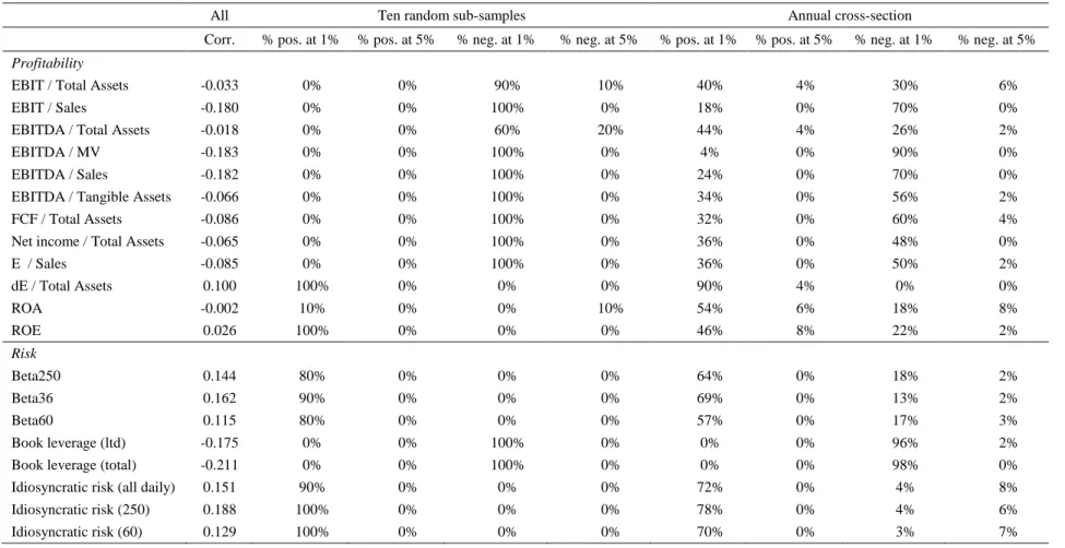
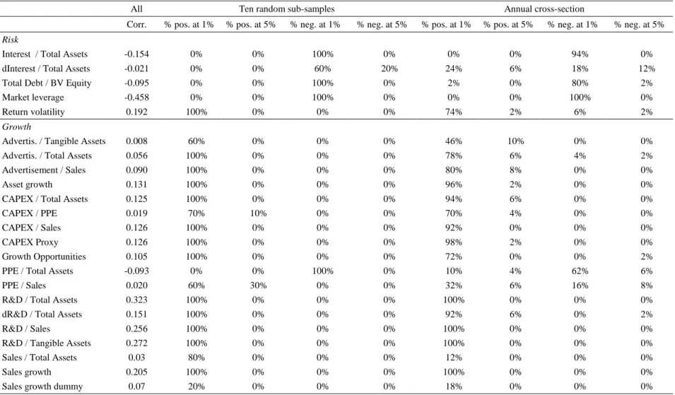
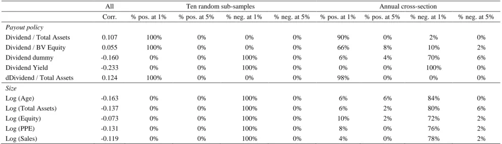
We conduct a univariate analysis similar to that in Frank and Goyal (2009) between each variable and the Tobin’s Q ratio. We compute the Pearson correlations and document how frequently they are statistically significant at the 1% (and 5%) level for negative and positive signs separately. This analysis gives a preliminary insight about the explanatory power of each variable and the stability of its corresponding sign.
[Table 1.2]
Table 1.2 shows the results. The first column is the correlation between each variable and firm value over the sample period. The next four columns show the proportion of correlations that are positive (respectively negative) and significant at the 1% and 5% (but not already significant at 1%) level in ten sub-samples. Column 6 to 9 report the proportion of correlation coefficients significant at the 1% and 5% (but not already significant at 1%) level for annual cross-sectional tests. The results indicate that the sign of pairwise correlations between the Q ratio and the proxies of profitability is not consistent. For instance, the negative correlation between ten profitability proxies and firm value is in contradiction with the theory. For nine of them, the correlation is more frequently negative than positive at the 1% level. Also in contradiction with the theory, measures of risk based on stock market prices (beta, idiosyncratic risk and volatility) are positively correlated with Q while, as expected, leverage proxies are
6 To have a balanced distribution of firm-years in ten sub-samples, we randomly divide the sample at each year and index them from 1 to 10, randomly. Then we aggregate them all by index to have the final 10 random sub -samples.
16
negatively correlated with Q. Two proxies (three) of the payout policy, the dividend yield and the dividend dummy (equal to one for firms paying dividends), are negatively (positively) correlated with Q. Reassuringly, the signs of the correlation between Q and the proxies for growth are consistently positive. Despite the ambiguous correlation predicted by the theory, we also obtain a consistent negative correlation for size. These preliminary results show that proxies of the core factors should not be considered in isolation.
1.3.2. Selecting the determinants of Tobin’s Q
Four model selection criteria have been employed in the literature: (a) Akaike Information Criterion (AIC, Akaike (1974)), (b) Bayesian Information Criterion (BIC, Schwartz (1978)), (c) Focused Information Criterion (FIC, Wei (1992) and (d) adjusted R2 to evaluate the explanatory power of the variables in a model.7 We use the BIC because of its popularity in literature; see e.g., Bossaert and Hillion (1999) and Frank and Goyal (2009). BIC is defined as:
2 log-likelihood log 4 BIC p n
where p is the number of variables in the model, and n the number of observations. Models with higher explanatory power generate a lower BIC. Given the high number of proxies, it is essential to remove those with low explanatory power.
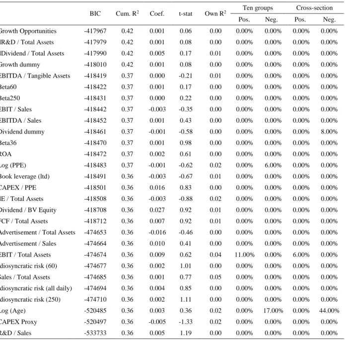
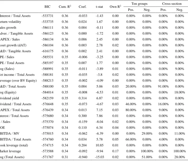
[Table 1.3]
For that purpose, we follow Frank and Goyal (2009) recursive procedure. First, we estimate the model with all proxies. In Table 1.3, columns 1 and 2, we report the BIC (-417967) and the adjusted R-square (42%). We then remove the proxy (Growth Opportunities) with the lowest t-statistic and estimate the regression of this proxy on Q. The corresponding coefficient (0.001), t-stat (0.06) and R-square (0%) are presented in Columns 3 to 5. Then, the model is re-estimated without the proxy with the lowest t-stat (Growth Opportunities). On the second row
17
(dR&D / Total Assets), column 1, we observe a slight drop in the BIC from -417967 to -417979. This procedure is iterated until the bottom of the table. The lowest BIC (-616175) is obtained when R&D / Tangible and all the explanatory variables below in Table 1.3 are included. At this stage, we still have nineteen explanatory variables in the model.
To reduce further the number of variables, the procedure described above is also repeated for both the ten groups and annually. At each test, when the lowest BIC is reached, we record the variables in the model and compute the proportion of groups for which a specific proxy has a positive (negative) coefficient and presents in the minimum BIC model. The variables that show most frequently in the lowest BIC model are assigned as core factors in the model.
Interestingly, there is at least one proxy, and a maximum of two, representing each core factor in the model. These proxies are EBITDA / Total Assets and EBITDA / MV for profitability, Market Leverage for risk, CAPEX / Total Assets and R&D / Total Assets for growth, Dividend / Total Assets for the payout policy and, Log (Total Assets) and Log (Equity) for size. For each core factor, we retain the proxy that has the highest stability in terms of sign. Therefore, EBITDA / MV and Log (Equity) are eliminated. Note that we keep two proxies for growth since they represent two different dimensions, i.e. CAPEX / Total Assets and R&D / Total Assets. The proxies included in our final specification are those present in minimum BIC model at least 50% of our sub-samples periods (either the ten groups or the annual cross-sections). They have also a sign that is consistent with the theory. Finally, they do not switch sign in the annual cross-sections or over the sub-samples. These findings are consistent with the literature. As indicated, EBITDA / Total Assets and Log (Total Assets) are the most frequent proxies for profitability and size in the surveyed papers, respectively. R&D / Total Assets and CAPEX / Total Assets are also among the most frequently used as proxies for growth. However, market leverage and dividend / Total Assets are not standard variables in firm valuation models.
18
1.3.3. Tobin’s Q baseline model
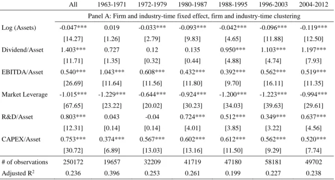
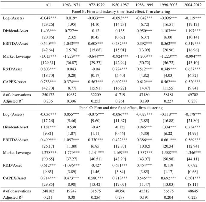
From the set of proxies selected in the previous section, we start our regression analysis of the baseline model (hereafter “BL”) by estimating equation (2) with firm and industry-time fixed effects. The t-statistics are adjusted for clustering at both firm and industry-time levels. Table 1.4, Panel A, displays results from OLS estimations of equation (2). Column 1 (“All”) to 7, report the results of the 1963-2012 period and the subsequent six eight-year sub-periods.
[Table 1.4]
Looking at the impact of the core variables in column 1, we notice that all of them have the expected sign and are statistically significant at the 1% level. The subsequent columns provide a slightly different message. While three core variables (EBITDA / Assets, Market Leverage and CAPEX / Assets) have the expected sign and are statistically significant at 1%, the remaining ones (Log(Assets), Dividend / Assets and R&D / Assets) are not significant at the usual level in three sub-sample periods. The 1972-1979 period shows a core variable (R&D / Assets) with the wrong sign but is not significant. The R-square is 23.6% for the 1963-2012 period and is between 19.9% and 39.6% for the remaining sub-periods.
In Table 1.4, Panel B, we examine whether clustering standard errors at the firm level only changes our inference. In the first and the subsequent columns, we remark that t-stat are higher (standard errors are too small). The two-way clustering really matters in our model. In Table 1.4, Panel C, we estimate the model with firm and time (instead of industry-time) fixed effect and cluster standard errors at the firm level. Globally, the statistical inference that we draw from the coefficients and their related t-stats are similar to that of Panel B. However, the R-square decreases when the whole sample and the sub-periods are considered.
1.3.4. An alternative Tobin’s Q (dynamic) model
As mentioned before, there is no variable selection for the Fama and French (1998) model (hereafter “FF”). We depart slightly from the original specification by introducing firm and
19
industry-time fixed effects. As for the baseline model, standard errors are clustered at the firm and the industry-time level. To check the robustness of our results, we re-estimate the model with firm and time fixed effect with standard errors clustered at the firm level.
[Table 1.5]
In Table 1.5, Panel A, column 1, we report the results for the 1963-2012 sample period. All the coefficients have the expected signs and are significant at the 1% level. Similar results are obtained for the six sub-sample periods. Panel B and Panel C confirm these results. Two limitations of this specification are noticeable. First, the number of observations is 30% lower because lead/lag variables require at least five consecutive years to be computed and, second, the explanatory power (R-square) is always lower than that of the baseline model (-4% for the 1963-2012 sample period). To explore further this issue, we decompose the variance as suggested by Coles and Li (2011). To facilitate comparison, we estimate both models on the same sample, i.e. the one used to estimate FF.
[Figure 1.1]
The observed variables of the BL and FF explain respectively 23% and 19% of the total variance. This is consistent with BL having a higher adjusted R-square since there are more independent variables in FF. The contribution of the firm fixed effects is high for both models (42% and 48% respectively) while the industry-time fixed effect is of a lower magnitude (9% and 8% respectively). To summarize the pros and cons: (a) BL has a higher in-sample explanatory power, (b) BL does eliminate unnecessarily observations and, (c) FF has parameter estimates that are more consistent over time.
The last step of our analysis consists in comparing directly the performance of both models. Since they are non-nested (i.e., they do not share the same independent variables), we use the statistical test developed by Vuong (1989). This test compares the log-likelihood functions of
20
both models. Under the null hypothesis (the log-likelihood functions are equal) the VMS statistics follows a standard normal:
1 , , 1 1 2 2 1 , , 1 , ~ 0,1 (5) n i FF FF i BL BL i N i FF FF i BL BL i n l l VMS FF BL N n l l n
where li BL FF,
BL FF
is the log-likelihood of the observation i under BL (FF), and n the numberof observations. A negative (positive) value of VMS indicates that BL (FF) should be preferred to FF (BL)
[Table 1.6]
Table 1.6 reports the value of the Vuong (1989) statistics (observed) and the related p-value for the whole sample and six sub-periods, and the ten groups. Over the whole sample, BL dominates and on the sub-periods BL is chosen three times, FF two times and two times the test is inconclusive at the critical level of 1%. For the ten groups, the Vuong statistics is always negative. Four and six (four) times it is significant at the 1% and 5% levels (inconclusive), respectively. To conclude our selection process, we choose BL because the sample is less affected to the survivorship bias, both models being comparable in terms of explanatory power.
1.4 Specification and power of the regression model
1.4.1. Description of the pseudo Monte Carlo simulationsTo examine the specific impact of the variable of interest on our BL model, we rewrite the model as follows:
, 0 1 , 6
i t t i Industry t it
Q
Int Γ ×F t
where
Q
i t, is the (Log) of Tobin’s Q, Intt
1 the variable of interest (coefficient of interest), t
21
on the variable of interest, we distinguish two cases: (a)
Int
tis a missing “continuous” variable in equation (6), and (b)Int
tis a treatment affecting some firms (treated) in the sample andleaving unaffected (controls) the remaining ones. The former case is the classic problem of the missing variable in a regression setting. The latter case is decomposed further based on whether the treatment is affecting specific firms: (b1) persistently after a common date but heterogeneously among firm-years (“Specific”), (b2) or constantly but reversible (“Reversible”). We do not explore settings in which the intensity of the treatment decays over time (e.g., autoregressive process AR(1) with a coefficient lower than 1).
1.4.1.1. Standard error estimation
As already shown in Section 1.3, standard error estimates have a strong tendency of being too small in our setting. Therefore, the null hypothesis is rejected too often. The potential corrections proposed in the literature are well known; see, e.g. Bertrand et al. (2004), Petersen (2009) and Gow et al. (2010). We use three different methods to estimate the standard errors. Our benchmark is the OLS standard errors without any adjustment. This benchmark is compared one-way clustered standard errors (firm level), two-way clustered standard errors (firm and the industry-time level), and the bootstrapped one- and two-way clustered standard errors as suggested by Cameron et al. (2008).
1.4.1.2. The specification and the power of the baseline model
Specification
To test whether the variable of interest has any impact on Tobin’s Q, we use Model (3). The null hypothesis is
H
0:
1
0
vs
1
0
. If the model is well specified, we should not reject the null in this setting. Therefore, to test the specification of the model, we generate 500 random panels, estimate the regression model for each panel and test whether we reject the null at 1%,
22
5% and 10% (α) significant level. The model is conservative if we reject the null lower than 500α times and anticonservative if we reject the null more than 500α. The control variables in our model is potentially skewd. This skewness increases the probability of Type I error in our test. Barber, Lyon, and Tsai (1999) address similar concern and refer to Sutton’s (1993) statement: “[Bootstrap] should be preferred to the t-test when the parent distribution is asymmetrical, because it reduces the probability of type I error in cases where the t-test has an inflated type I error rate and it is more powerful in other situations.”. Hence, we estimate the probability of rejection on both sides of the distribution.
More specifically, to generate a panel, we randomly choose a year t between 1963 and 2005. On year t, we randomly choose 500 firms with replacement. To calibrate our simulations with the surveyed research, we explore additional dimensions. We select an eight-year panel data from year t to t+7. This panel length corresponds to the median of the surveyed papers; see Table 1.1. Some firms may not exist for the whole period. As a result, our panels are unbalanced. We conduct our tests for each type of treatments separately. For “Reversible” treatment, at each iteration, after generating panel from a randomly chosen year and firms, we assign Treatment = 1 to random firm-years in our sample. We conduct separate tests when 20%, 40% and 60% of
firm-years in the panel are treated. For “Continuous” variable, at each iteration we generate random numbers from a normal distribution with zero mean and variance equal to 1%, 2.5% and 5% of the variance of the Log (Q) in our randomly generated panel. These marginal variances are in line with those of control variables in our model. Last, for “Specific” treatments, we generate random numbers with similar procedure explained for “Continuous” treatments. Then, we assign these numbers to random firms after a random year in the period of the panel. This test is repeated for different portion of treated firms, i.e. 20%, 40% and 60% of the firms in each panel.
23
We turn our attention to the power of the model (Type II). We follow the methodology applied in Barber et al. (1999). For “Reversible” and “Specific” treatments, after generating the panel, we manipulate firm value by artificially adding ±20%, ±15%, ±10%, and ±5% of the firm values for treated firms. For “Continuous” treatment, we add ±20%, ±15%, ±10%, and ±5% of
Intt to Log (Q) as abnormal firm values. Similar to specification test, we focus on the coefficient
of the variable of interest and test the null hypothesis of
10
10
for negative (positive) abnormal firm values at 1%, 5% and 10% (α) statistical significance levels. The rejection rate of the null gives the power test.For both specification and power tests, we run the model with firm and industry-time fixed effects and estimate the standard error of the coefficients robust to heteroskedasticity and autocorrelation clustered at firm level. We also estimate the model with firm and industry-time clusters. Bootstrapping with 200 times resampling is also conducted for these tests. Finally, we estimate the model with random effects and clustering at firm level.
1.4.2. Results
Table 1.7 reports the results of specification tests for “Reversible” treatments. The numbers in the table show the percentage of rejection of the null at corresponding statistical significance levels of 1%, 5% and 10%. As indicated in the table, the model is anticonservative when 20% of the firms are treated. It might be the result of high number of zero values for treatments that generates a strong autocorrelation for this variable. This autocorrelation results in underestimation of the standard errors for variable of interest. In this context, we observe that the additional layer of clustering at industry-time level improves the performance of the model but not significantly. Bootstrapped resampling exacerbates the underestimation of the standard errors for this type of treatment. Last, we observe that the performance of the random effect model is identical to fixed effect in specification tests. Moreover, our results reveal that increasing the number of treated firms significantly improves the performance of the model. The
24
model is almost well specified when 40% of firms are treated and is almost conservative when the number of treated firms is 60%. In fact, for higher number of treated firms, we have less clustered zero values and consequently less autocorrelation in variable of interests. When the number of treated firms are increased, the advantage of double clustering vanishes. Similar to previous results, there is no improvement in the results in bootstrap and random effect models. Result show that when the number of treated firms are low and the impact of treatment is constant, researchers should be cautious in interpreting the results in which the null hypothesis could be rejected based on the nature of the data rather than the economic impact of the treatment.
[Table 1.7]
Results of power test of the model for “Reversible” treatments are reported in Table 1.8. As demonstrated in the table, when Log (Q) is increased or decreased 10% or more, the model identifies the abnormal firm values in 100% of the tests. For 5% abnormal firm values, the model still performs well in more than 80% of the tests. Similar to results for specification test, there is no significant difference in the performance of the model when we apply double clustering, bootstrap or random effects in our model.
[Table 1.8]
Furthermore, we conduct our tests for “Continuous” variable of interests. Specification tests are reported in Table 1.9. Compared to “Reversible” treatment, we observe a significant improvement in the model specification which is well specified when the variance of the variable of interest is 1% of that of Log (Q). The model becomes more conservative when the marginal variance increases to 2.5% and 5%. It is natural since we have an increase in standard deviation of coefficient and consequently less rejection. We should note that the simulated variable of interest does not have autocorrelation in this test that explains the improvement in specification tests compare to “Reversible” treatments. Similar to previous test, increasing the layer of
25
clustering as well as bootstrap and random effect do not improve the performance of the model for “Continuous” variable of interest.
[Table 1.9]
In Table 1.10, we report the results for power test of the model. Similar to specification test, we conduct our analysis with different variance of variable of interest, i.e. 1%, 2.5% and 5% of variance of the Log (Q) as well as different level of abnormal Q. In all tests, the model rejects the null hypothesis. In summary, this model can explain the impact of continuous variables of interest (without autocorrelation) on firm value with high reliability and confidence.
[Table 1.10]
In the last step, we estimate the model for “Specific” treatments. Our test varies in two dimensions in this step. We conduct our test on different portion of treated firms – i.e. 20%, 40% and 60% of the firms – with variances of variable of interest equal to 1%, 2.5% and 5% of the Log (Q). Results of specification tests are presented in Table 1.11. Independent from portion of treated firms, an increase in variance of the variable of interest improves the performance of the model. In terms of portion of treated firms, the model is almost well specified when 20% of firms are treated. When this portion increases to 40% and 60%, we observe that the model becomes more conservative. Similar to previous tests, double clustering, bootstrap or random effect do not improve the specification of the model.
[Table 1.11]
In terms of power of the model, we report the results for portion of firms treated for 20%, 40% and 60% in Panels A to C in Table 1.12 respectively. As presented, in all three portion of treated firms, the power of the model increases when the abnormal treatment of the firm value decreases. This trend looks counterintuitive at first glance. However, the variance of the variable of interest explains this trend. In fact, abnormal values are applied exclusively to treated firms. It means
26
that the impact of the marginal increase on the variance of variable is larger than its impact on its average value. It results in the increase of standard error of estimates and consequently the model fails to identify the abnormal increase. Based on this explanation, we should observe an increase in the power of the model when the portion of treated firms increases. As reported in Tables B and C, when the portion of treated firms increases to 40% and 60%, the performance of the model increases significantly. At the limit, when all firms are treated, we have a continuous treatment in which the model identifies abnormal Qs in all tests, as reported in Table 1.10. Consistent to previous results, double clustering, bootstrap and random effect models do not show any improvement in performance of the model. Overall, researchers should interpret the results of “Specific” treatments in panels cautiously when the variance of the variable of interest is significantly lower than that of firm value.
[Table 1.12.A] [Table 1.12.B] [Table 1.12.C]
1.5 Conclusion
Firm value theories describe profitability, risk and growth options as the main elements of firm value. In this study, we review several papers in firm value literature. We identify proxies used for the profitability, risk and growth separately. We also find that the majority of studies evaluate the impact of dichotomy variables in firm value. These dichotomy variables are generally random over firms and time (“Reversible” treatments) but there are also researches work on variables persistent for specific firms after a certain date (“Specific” treatment). Using all proxies used in reviewed papers, we apply Bayesian Information Criterion (BIC) methodology and identify Log (assets), EBITDA / Total Assets, market leverage, CAPEX / Total Assets, R&D / Total Assets, and Dividend / Total Assets as the core factors in firm value.
27
We test the power and specification of the model based on these variables. Our tests reveal that when the variable of interest is “Continuous” without autocorrelation, the specification and power of the model is ideal. In “Reversible” treatments, the specification of the model is sensitive to the portion of treated firms due to its impact on the autocorrelation in non-treated firms. This sensitivity does not exist for power of the model. Alternatively, the power of the model is sensitive to the magnitude of the abnormal firm values. In particular, the power of the model significantly reduces when the abnormal firm value is lower than 5% in absolute values. For “Specific” treatment, the performance changes over two dimensions. The specification, improves when the variance of the variable of interest increases. When the portion of treated firms is 20%, the power of the model is highly sensitive to the magnitude of the abnormal firm value. This sensitivity diminishes when the portion of treated firms increases to 40% and 60%. In summary, researchers can rely on the result of the model for “Continuous” treatment with low autocorrelation for testing the hypothesis. However, the results should be cautiously interpreted when treatments are not continuous. The portion of treated firms as well as the variance of the treatment should be taken into consideration for interpretation of the results.
REFERENCES
Adam, R., Ferreira, D., 2009. Women in the boardroom and their impact on governance and performance. Journal of Financial Economics 94, 291-309.
Agrawal, A., Knoeber, C., 1996. Firm performance and mechanisms to control agency problems between managers and shareholders. Journal of Financial and Quantitative Analysis 31, 377-397.
Ahern, K., Dittmar, A., 2012. The changing of the boards: The impact on firm valuation of mandated female board representation. Quarterly Journal of Economics 127, 137-197. Akaike, H., 1974. A new look at the statistical model identification. IEEE Transactions on
Automatic Control 19, 716-723.
Allayannis, G., Weston, J.P., 2001. The use of foreign currency derivatives and firm market value. Review of Financial Studies 14, 243-276.
28
Anderson, R., Reeb, D., 2003. Founding family ownership and firm performance: Evidence from the S&P 500. Journal of Finance 58, 1301-1327.
Baek, J.-S., Kang, J.-K., Suh Park, K., 2004. Corporate governance and firm value: Evidence from the Korean financial crisis. Journal of Financial Economics 71, 265-313.
Bakshi, G., Chen, Z., 2005. Stock valuation in dynamic economies. Journal of Financial Markets 8, 111-151.
Barber, B., Lyon, J., 1996. Detecting abnormal operating performance: The empirical power and specification of test statistics. Journal of Financial Economics 41, 359-399.
Barber, B., Lyon, J., 1997 JFE
Barth, M., Clinch, G., 1998. Revalued financial, tangible, and intangible assets: Associations with share prices and non-market-based value estimates. Journal of Accounting Research 36, 199-233.
Bartram, S., Brown, G., Conrad, J., 2011. The effects of derivatives on firm risk and value. Journal of Financial and Quantitative Analysis 46, 967-999.
Bebchuk, L., Cohen, A., 2005. The costs of entrenched boards. Journal of Financial Economics 78, 409-433.
Berk, J., Green, R., Naik, V., 1999. Optimal investment, growth options, and security returns. Journal of Finance 54, 1553-1607.
Bertrand, M., Duflo, E., Mullainathan, S., 2004. How much should we trust differences-in-differences estimates? Quarterly Journal of Economics 119, 249-275. Bhojraj, S., Lee, C., 2002. Who is my peer? A valuation based approach to the selection of
comparable firms. Journal of Accounting Research 40, 407-439.
Billett, M.T., Mauer, D.C., 2003. Cross-subsidies, external financing constraints, and the contribution of the internal capital market to firm value. Review of Financial Studies 16, 1167-1201.
Black, B., Kim, W., 2012. The effect of board structure on firm value: A multiple identification strategies approach using Korean data. Journal of Financial Economics 104, 203-226. Bossaerts, P., Hillion, P., 1999. Implementing statistical criteria to select return forecasting
models: What do we learn? Review of Financial Studies 12, 405-428.
Cameron, C., Gelbach, J., Miller, D., 2008. Bootstrap-based improvements for inference with clustered errors. Review of Economics and Statistics 90, 414-427.
Campa, J.M., Kedia, S., 2002. Explaining the diversification discount. Journal of Finance 57, 1731-1762.
29
Carter, D., Rogers, D., Simkins, B., 2006. Does hedging affect firm value? Evidence from the US airline industry. Financial Management 35, 53-86.
Chung, K., Pruitt, S., 1994. A simple approximation of Tobin's Q. Financial Management 23, 70-74.
Coles, J., Li, Z., 2011. An empirical assessment of empirical corporate finance. http:// papers.ssrn.com/abstract=1787143
Cronqvist, H., Nilsson, M., 2003. Agency costs of controlling minority shareholders. Journal of Financial and Quantitative Analysis 38, 695-720.
Daines, R., 2001. Does Delaware law improve firm value? Journal of Financial Economics 62, 525-558.
Daske, H., Hail, L., Leuz, C., Verdi, C., 2008. Mandatory IFRS Reporting around the World: Early Evidence on the Economic Consequences. Journal of Accounting Research 46, 1085-1142.
Denis, D., Denis, D., Yost, K., 2002. Global diversification, industrial diversification, and firm value. Journal of Finance 57, 1951-1979.
Dey, A., 2008. Corporate governance and agency conflicts. Journal of Accounting Research 46, 1143-1181.
Dittmar, A., Mahrt-Smith, J., 2007. Corporate governance and the value of cash holdings. Journal of Financial Economics 83, 599-634.
Dong, M., Hirshleifer, D., 2005. A generalized earnings based stock valuation model. The Manchester School 73, 1-31.
Durnev, A., Morck, R., Yeung, B., 2004. Value enhancing capital budgeting and firm specific stock return variation. Journal of Finance 59, 65-105.
Evans, J., Nagarajan, N., Schloetzer, J., 2010. Turnover and Retention Light: Retaining Former CEOs on the Board Journal of Accounting Research 48, 1015-1047.
Fahlenbrach, R., 2009. Founder-CEOs, investment decisions, and stock market performance. Journal of Financial and Quantitative Analysis 44, 439-466.
Fahlenbrach, R., Stulz, R., 2009. Managerial ownership dynamics and firm value. Journal of Financial Economics 92, 342-361.
Faleye, O., 2007. Classified boards, firm value, and managerial entrenchment. Journal of Financial Economics 83, 501-529.
Fama, E.F., French, K.R., 1992. The cross-section of expected stock returns. Journal of Finance 47, 427-465.
30
Fama, E., French, K., 1998. Taxes, financing decisions, and firm value. Journal of Finance 53, 819-843.
Fang, V., Noe, T., Tice, S., 2009. Stock market liquidity and firm value. Journal of Financial Economics 94, 150-169.
Fauver, L., Houston, J., Naranjo, A., 2003. Capital market development, international integration, legal systems, and the value of corporate diversification: A cross-country analysis. Journal of Financial and Quantitative Analysis 38, 135-158.
Fauver, L., Naranjo, A., 2010. Derivative usage and firm value: The influence of agency costs and monitoring problems. Journal of Corporate Finance 16, 719-735.
Fazzari, S., Hubbard, R.G., Petersen, B.C., 1988. Financing constraints and corporate investment. Brookings Papers on Economic 19,141–95.
Fernandez, P., 2013. Cash flow is a fact. Net income is just an opinion. http://papers.ssrn.com/sol3/papers.cfm?abstract_id=330540
Fich, E.M., Shivdasani, A., 2006. Are busy boards effective monitors? Journal of Finance 61, 689-724.
Frank, M.Z., Goyal, V.K., 2009. Capital structure decisions: Which factors are reliably important? Financial Management 38, 1-37.
Frésard, L., Salva, C., 2010. The value of excess cash and corporate governance: Evidence from US cross-listings. Journal of Financial Economics 98, 359-384.
Gompers, P., Ishii, J., Metrik, A., 2003. Corporate governance and equity prices. Quarterly Journal of Economics 118, 107-155.
Gormley, T., Matsa, D., 2014. Common errors: How to (and not to) control for unobserved heterogeneity. Review of Financial Studies 27, 617-661.
Gozzi, J., Levine, R., Schmukler, S., 2008. Internationalization and the evolution of corporate valuation. Journal of Financial Economics 88, 607-632.
Gow, I., Ormazabal, G., Taylor, D., 2010. Correcting for cross-sectional and time-series dependence in accounting research. Accounting Review 85, 483-512.
Gurun, U., Butler, A., 2012. Don't believe the hype: Local media slant, local advertising, and firm value. Journal of Finance 67, 561-598.
Hanson, S., Sunderam,A., 2012. The variance of non-parametric treatment effect estimators in the presence of clustering. Review of Economics and Statistics 94, 1197-1201.
Hastie, T., Tibshirani, R., Friedman, J., Franklin, J., 2005. The elements of statistical learning: data mining, inference and prediction. The Mathematical Intelligencer 27, 83-85.