HAL Id: hal-00973093
https://hal-sciencespo.archives-ouvertes.fr/hal-00973093
Preprint submitted on 3 Apr 2014
HAL is a multi-disciplinary open access archive for the deposit and dissemination of sci-entific research documents, whether they are pub-lished or not. The documents may come from teaching and research institutions in France or abroad, or from public or private research centers.
L’archive ouverte pluridisciplinaire HAL, est destinée au dépôt et à la diffusion de documents scientifiques de niveau recherche, publiés ou non, émanant des établissements d’enseignement et de recherche français ou étrangers, des laboratoires publics ou privés.
Voter Turnout and Fiscal Policy
Raphaël Godefroy, Emeric Henry
To cite this version:
Voter Turnout and Fiscal Policy
Raphael Godefroy and Emeric Henry∗
November 14, 2011
Abstract
Though a large literature on the determinants of turnout has flourished, there is scant evidence on the causal impact of turnout on policies implemented in practice. Using data on French munic-ipalities and instrumental variables for turnout based on temperature and influenza variations, we show that a one percent increase in turnout decreases on average the municipalities’ yearly budget by 1.5 percent. This is mostly due to a decrease in spending on equipment or personnel. We show that this could be the result of a negative effect of turnout on the strength of the incumbent’s majority combined with the fact that the incumbent promises higher budgets. We argue, in the context of a theoretical model, that these different facts could be natural consequences of the well documented incumbency advantage.
1
Introduction
Voter turnout has consistently been decreasing in most Western democracies over the last 40 years. For instance, turnout in the first round of French municipal elections dropped from 78.2 in 1965 to 66.5 in 2008.1
Many argue that this is a worrying sign for the health of our democracies. Although a large literature examines the determinants of turnout, little is known on the effect of turnout on policies implemented in practice.2
We fill this gap by examining the impact of turnout on fiscal policy, using data on French municipalities.
A large literature in political science addresses the question of whether those who actually vote are representative of the larger population. Based on survey evidence, they find either no significant
∗Paris School of Economics, 48 boulevard Jourdan, 75014 Paris and Sciences Po, department of Economics, 28 rue
des Saint Peres, 75007 Paris.
1The corresponding turnout figures for US presidential elections are 61.9 in 1964 and 57.37 in 2008 and the drop is
much larger for midterm elections.
2Several papers, discussed below, study the effect of enfranchisement laws, which affect the number of eligible voters,
differences (see the seminal paper by Wolfinger and Rosenstone 1980), or evidence suggesting that non voters tend to be poorer and may favor more public spending (e.g. Leighley and Nagler 2007 for the US, Perrineau 2007 for France). Our work, using revealed preferences observed in the data, provides new evidence, not on the overall population of non voters, but on the marginal voters with intermediate level of voting costs, who turn out to vote or not depending on specific conditions.
We show that these voters are significantly different from the rest of the voting population in terms of preferences for spending. Indeed, an increase in turnout has a significant and large negative impact on municipalities’ budgets with an elasticity in the order of -1.5, suggesting that the marginal voter is on average in favor of lower spending. Furthermore, we construct a model and provide arguments that suggest that this may not reflect an intrinsic correlation between voting costs and budgetary preferences, but could be the result of electoral promises endogenously making the marginal voter vote against the spending associated to these promises.
Compulsory voting is a frequently discussed way of addressing the problem of decreasing turnout, and is implemented in several countries. However, the studies mentioned above, and evidence from simulations (Citrin et al. 2003), suggest that introducing mandatory voting might have little impact in terms of implemented policies.3
Our work highlights the fact that policies to increase turnout other than mandatory voting, such as information campaigns or reforms facilitating voter registration, might actually have much larger impacts on implemented policies, and thus on welfare, since they affect those marginal voters that are at the limit between voting and not voting.
Two main problems have to be overcome to establish a causal effect of turnout on policies. First, turnout is endogenous. It is correlated with municipal characteristics, such as the number of residents of a municipality, their average income etc., that could impact municipal finances. We overcome this problem by using two different instruments for turnout, one based on weather conditions and the other on flu incidence.
Second, the rules that govern the elections of public representatives, set their collective deci-sion procedures, and delimit their power, differ across nations, and may substantially vary across infra-national polities within a nation.4
This heterogeneity impedes the comparison of policies across governments and requires to control for a wide array of variables in order to test the impact of turnout on policies.
3There is also a body of theoretical work discussing the question of whether compulsory voting is welfare enhancing
that obtains ambiguous results (see B¨orgers 2004, Krasa and Polborn 2009)
4This is the case for US municipalities, for instance. Municipal government can take the form of either mayor-council
To overcome this second problem, we take advantage of one particularity of French local insti-tutions: their homogeneity. Due to a highly centralized system, all municipalities are subject to the same national law, that sets the election date, election rules as well as the role of municipal councils. We thus use longitudinal data on fiscal policy and electoral outcomes that span the years 1998-2010, for a sample of around 4000 municipalities, located in the Western part of France.5
Two municipal elections took place over this period, one in March 2001, the other in March 2008.
We propose the two following instruments for turnout. First, we use average temperature on election day, relative to temperature the day before. Higher relative temperatures on election day have a negative impact on turnout, significant for the election of 2001. Second, we use an instrument that measures the speed of progression of the flu epidemic in the weeks preceding the election day. A faster progression has a negative effect on turnout, significant for the 2008 election.
We do not claim that we have identified universal instruments that will always be powerful predictors of turnout. In fact, these effects are due to unusual weather conditions in 2001, and an unusually severe flu season in 2008, that took place at the time of - or just before - the elections in our area of study. These conditions were documented in several articles of the local newspaper, which we mention below, and confirmed by an examination of our data.6
The idea of the instrument based on weather is that when a relatively nice Sunday follows a relatively cold Saturday, potential voters will be tempted to engage in outdoor activities rather than turnout to vote. Thus this instrument is unlikely to work in a country such as the US where elections are run on a weekday. Nevertheless, in the context we study, these instruments turn out to be powerful predictors of turnout, and we find very robust effects of turnout on public finances, regardless of the instrument we use.
Our identification assumption is that, controlling for observable municipal characteristics, our instruments are uncorrelated with the unobservable factors that affect the trend of the fiscal outcomes we examine. In fact, we find that neither instrument is correlated with the municipal characteristics that we do actually observe, which include the main determinants of municipal finances. More im-portantly, when we restrict our sample to observations covering the years before a municipal election year, we find no correlation between any given fiscal outcome and the instrument for turnout for that election, and no impact of the instrument on the change in any given fiscal outcome after any arbitrary year.
Our first main result establishes that turnout has a significant negative impact on the revenues
5Comprehensive electoral data, recorded by a local newspaper, are available for this geographic area only.
6The average temperature on the elections weekend in 2001 was around 10◦F above average, whereas the prevalence
of the municipality. A one percent increases in turnout, decreases yearly revenues in the order of 1.5 percent. This represents an average decrease of 18 euros per capita per year for a one percent increase in turnout. It is remarkable that the result does not seem to depend on the origin of the variation in participation: regardless of whether temperature or flu caused this variation in turnout, the effect is of the same size and goes in the same direction.
These estimates can also be used to derive estimates of voting costs. Indeed the main result can also be expressed in a different way: an additional vote decreases on average the yearly budget by 2.2 euros. Thus the maximum expected benefit from voting of the marginal voter is 2 .2 euros per year for 6 years, that is the length of a term, since in the worst case scenario the voter would not have benefited at all from this extra spending. This figure is an upper bound on voting costs, net of non financial benefits such as a warm glow from performing one’s civic duty.
On the spending side, our second result is to show that this decrease is due mostly to a fall in spending on investments in equipment (such as building schools or roads) or a decrease in spending on personnel. The effect can be large: a one percent increases in turnout, decreased spending on equipment by at least 3 percent after the 2001 elections. We also find that turnout has no systematic impact on taxes.
The effect of turnout on municipal finances, that turns out to be large, is puzzling. We propose a mechanism, that appears to be supported by further evidence.7
We argue that these effects are a consequence of a subtle electoral interaction. Indeed we establish that an increase in turnout decreases the probability that the incumbent majority has a large share of the municipal council. If it is the case that the incumbent proposes and implements a higher budget and larger spending on equipment, then our main empirical results naturally follow.
This difference between the incumbent’s and the opposition’s electoral platforms can be seen as a natural consequence of a well documented fact called the incumbent advantage. It has been systematically established, mostly for American elections, that the incumbent has a significantly higher probability of being elected. It appears to be true in our data where 65% of incumbent majority coalitions are reelected. This advantage means that the incumbent mayor is less accountable. Thus, in a situation where he has a relative preference for a higher budget compared to voters, he can propose more spending and still preserve a good chance of being reelected.
To fix ideas, consider the following setting, which we study in detail in the theoretical model of section 5. Suppose that an election is run, based on binding campaign promises, where both an
incumbent and the opponent he is facing have, on top of regular spending on public goods, a preference for spending on particular pet projects, such as a school or a new townhall. These pet projects are supported by less than a majority of voters, but if proposed, cause the voters who favor them to turnout for sure. Consider moreover the following incumbency advantage: the incumbent can fund his preferred project at a lower cost than his rival (for instance he has easier access to subsidies or to the credit market).
In such a setting, the opposition candidate will never propose his pet project and his proposed budget will always be smaller than that of the incumbent. The key is that if both candidates propose their pet projects, voters who dislike both of these plans will still turn out to vote for the incumbent since he can fund his project at a lower cost. The most natural outcome is then that only the incumbent proposes his preferred project. Voters that support it turn out for sure while other voters, who vote against the incumbent if they come and vote, will only turnout if voting costs are low enough. Thus, a decrease in voting costs increases turnout, decreases the probability that the incumbent is reelected, and incidentally decreases the average budget implemented by the winner of the election (we show in Godefroy and Henry 2011 that these results also hold in a more general setting). In our model, the effect of turnout on fiscal policy is independent of the source of variation in turnout, which is consistent with our empirical results.
We insist on the fact that we can make no definitive welfare claims on the effect of higher turnout. Indeed it is not currently possible to establish whether budgets are too low or too high. Note that it is not even obvious in the theoretical context we outlined. If the preferences of the few voters who like the incumbent’s pet project are sufficiently strong, then implementing such a project is welfare enhancing and increasing turnout would have a negative impact on welfare.
Related Literature. There is a growing theoretical literature examining whether making voting compulsory is welfare enhancing. B¨orgers 2004 shows that, in a situation where the expected number of supporters for the two candidates is equal in the population, compulsory voting is welfare reducing. Krasa and Polborn 2009 point out that the result depends on the assumption that the general elec-torate is equally split. If this is not the case, mandatory voting will typically be welfare improving. Note that both papers consider mandatory voting as a decrease in the cost of voting, which corre-sponds exactly to the case we examine empirically of a shock on weather or flu incidence. Citrin et al (2003), simulate the outcome of elections as if everyone had voted, fixing the preferences of non voters based on their socioeconomic profile and suggest mandatory voting would not affect the outcome.
These papers build on the large theoretical literature on rational turnout (see survey by Dhillon and Peralta 2002 and Feddersen 2004). Most models in the game theoretic branch of the literature assume that potential voters make a rational decision comparing their cost of voting to the probability of being pivotal in the election, conditional on the other voters’ strategies. We use the same type of model of turnout in section 5. This leads to the paradox of voting in large elections since the probability of changing the outcome becomes negligible. To judge how large this paradox is, we need to have a rough idea of voting costs, which is a byproduct of our results.
There is a large empirical literature studying the determinants of turnout that we will not attempt to fully survey here. One of the key findings of this literature, though, is that, on top of classical ex-planations based on socioeconomic background, information is one of the main determinants of voting. For instance, Banerjee, Kumar, Pande and Su 2010, show in the context of an experiment in India, that access to information on candidates significantly increases turnout. The effect of information is also reflected in the fact that higher level of education can lead to higher turnout rates (causal link established for instance in Milligan et al. 2003) and in the literature on the influence of the media: Stromberg 2004 shows that regions with higher radio penetration had higher levels of turnout, and Gentzkow 2006 shows the opposite effect of television (television making people less informed by mov-ing them away from more traditional media) in the US. Enikolopov, Petrova and Zhuravskaya 2011, however, find no significant effect of the presence of an independent TV channel in Russia. Other factors can have sizable effect on turnout: Washington 2006 finds that the presence of Black Democrat candidates on the ballot has substantial and significant positive effects on turnout, both among Black and White voters.
Several papers study the effect of legal changes that led to an increase in turnout. Most of them (Husted and Kenny 1997, Lott and Kenny 1999, Miller 2009) examine the impact of the extension of voting rights, such as women’s enfranchisement in the US, and find that it caused an increase in welfare spending, especially in public health policies. Similarly, Fujiwara 2010 finds similar results for Brazil through the study of the introduction of technologies to facilitate voting for less educated individuals. Although related our work differs substantially from these studies. First, they cannot distinguish the effect of the change in the size of the eligible population from the actual impact of voter turnout itself. More importantly, these changes modified the number of voters in a way that politicians could anticipate, and, in some cases, encouraged by supporting enfranchisement laws. Here, our focus is different since we are interested in variations of turnout that cannot be anticipated more than a few weeks before the elections.
To the best of our knowledge, there is no study testing directly the impact of voter turnout on implemented policies. The effect of turnout on political outcomes is of course of wide interest in the political science literature. There are debates discussing whether higher turnout tends to give an advantage to Democrats. Recently, a few studies have started addressing the endogeneity problem inherent in the early literature, in particular instrumenting turnout with rainfall. Gomez et al. 2007 show that lower turnout increases the Republican party’s vote share in national elections. Hansford and Gomez 2010, who also use rainfall as an instrument, confirm this finding and also show that an increase in turnout decreases the vote share of the incumbent. Gentzkow, Shapiro and Sinkinson 2011 find no impact of newspaper entry on incumbents’ probability of reelection. However, their empirical strategy relies on shocks on turnout that could be anticipated by candidates and voters. More importantly, these studies examine the impact of turnout on political outcomes and not on actual policies implemented.
Some empirical papers address the effect of political variables on local public finances. Enikolopov and Zhuravskaya 2007 find that the effect of decentralization in Russia critically depends on whether local representatives are elected or appointed. Using data on local governments in Sweden, Pettersson-Lidbom and Tyrefors 2011 find that representative democracy increased both political participation and size of government, relative to direct democracy. In the US, Ferreira and Gyourko 2009 show that partisanship, i.e the fact that the mayor belongs to the Democrat or the Republican party, does not have an impact on policy outcomes (size of government, tax rates) at the municipal level in US cities. We argue that the incumbent effect could be at the source of the results we observe. There is a large literature attempting to establish and explain this incumbent effect. For instance Lee 2008 using a regression discontinuity approach, shows that an incumbent who was barely elected in the previous election has a significantly higher chance of being elected in the next election than his rival. There are also numerous papers that we review in section5 explaining this advantage. We provide a slightly different story than those typically suggested, since the source of incumbency advantage is in our model (supported by some empirical evidence) that the incumbent has better access to subsidies and to the credit market.
The remainder of the paper is organized as follows. In Section 2we present the data and institu-tional background. In Section3we expose our identification strategy. Results are presented in section 4 and interpreted in the context of a particular model in section 5. Tables and proofs are presented in the appendix B.
2
Data and Institutional Background
Since the French Revolution, in 1789, the French territory has been divided in municipalities, the smallest administrative unit in the country. France now counts 36682 such municipalities8
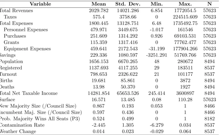
(compared to roughly 80000 in the whole of the EU). Both the rules that govern elections and the duties of the elected officials are set in national law and apply uniformly across the territory. In this section, we present some institutional background on French municipalities and information on the data we use. All summary statistics are in table1. We also document the specific weather and flu spread conditions in 2001 and 2008 respectively.
Our data span the years 1998 to 2010. Two municipal elections took place over this period, in 2001 and 2008, on the same days in all municipalities. Municipal elections have two rounds in France, the second round occurring one week after the first. The first round of the 2001 elections was on Sunday, March 10th, the first round of the 2008 elections was on Sunday, March 9th.
2.1 Electoral system and data on elections
Municipalities are governed by a municipal council whose members are elected through direct universal suffrage. Any adult above 18 living in the city, French or EU national, can register to vote. Elections, organized on the same days nationwide, comprise two rounds, which are held at a week interval, always on a Sunday. The electoral system of a town, and the size of its municipal council, depend on its population. Below 3500 inhabitants, the electoral system follows a first-past-the-post voting method: every voter can give at most one vote to any arbitrary number of candidates smaller than the number of seats. The candidates fill the available positions in order of highest vote.9
Above 3500 constituents, a degree of proportionality is introduced. The size of the council and other information on French local institutions is provided in Appendix A.
The municipal councilmen then elect one among themselves to serve as mayor (not necessarily the one that got the highest number of votes in the municipal election). The mayor is the agenda setter and the enforcer of decisions passed at the council. The municipal council must meet at least once every three months and deliberations are open to the public. Any proposal, including the city’s budget, must be approved by a majority of councilmen.
8as of January 1st 2010
9a candidate can be elected in the first round only if more than half voters and at least a quarter registered voters
Data on municipal elections come from two sources, the Ministry of Home Affairs, and the daily newspaper Ouest France, which covers the Western part of France. For every municipality and elec-tions year, we know the level of voter turnout, the name of the incumbent mayor, the names of all the members of the newly elected council, including the newly elected mayor (source: Ouest France). Although candidates can run independently in towns with less than 2500 inhabitants, most actually belong to a coalition and the data from Ouest France mention for each candidate the coalition he/she belongs to. These coalitions are usually not, or very loosely, related to one the main parties active at the national level.
Given the importance of detailed electoral data to understand the mechanism through which turnout influences policies, we restrict our analysis to the area covered by the newspaper, i.e to the Western part of France. We define the turnout in some municipality and some election, as the number of individuals who voted in the first round of that election.
2.2 Municipal finances
The main areas of competence of French municipalities, set in national legislation, have been roughly stable since 1884 and more importantly, by and large, do not depend on the city size. Apart from administrative duties (such as keeping the register of deaths, births...), the municipality is in charge of providing services such as lighting, water and most importantly primary school education, of maintaining public buildings and roads and of deciding new investments (such as public housing, industrial zones, primary schools...).
The main sources of revenues are taxes, subsidies and loans.10
The municipal council fixes the tax rate of three main categories of taxes: tax on homeowners, tax on inhabitants and professional taxes. It obtains subsidies from other local governments, or from the state. A share of these subsidies is based on well specified factors, such as the population or the surface of the municipality, but another is more discretionary. Finally, some municipalities contract loans. Note that they do not have to obtain authorizations from higher levels of government to sign a loan but that this additional money can only be used to finance new investments.11
Although municipal councils have a high level of autonomy, their accounts come under close scrutiny. The accounts are examined yearly by the an independent agency made up of civil servants
10By convention, municipal revenues include loans.
11In particular the townhall has to be able to finance, using collected taxes and the DGF, all the “current activities”
(paying salaries, maintaining equipment..). In the municipal accounts, the total of Produits de Fonctionnement needs to cover the Charges de Fonctionnement
not subject to political fluctuations, so that misappropriation of funds does not seem of concern here.12
Data on municipal finances were provided by the French Ministry of Finances for the period 1998-2010. For every year and municipality in our sample, we observe the total amount of municipal revenues and expenses. On the revenue side we can distinguish specifically the amount of taxes. Unfortunately given the level of aggregation of our data, we cannot distinguish subsidies from loans. In terms of spending we can observe small purchases (computer, gas for vehicles), larger equipment (roads, schools) and personnel expenditures.
2.3 Data on municipal characteristics
Data on other municipal characteristics come from the Institut National des Statistiques et Etudes
Economiques, roughly equivalent to the Census Bureau in the US and the French Ministry of Finances.
For every municipality, we observe the number of primary residents, “population” hereafter, which was measured in the two last censuses that took place respectively in 1999 and 2007. In addition, we use data on the total net taxable income of primary residents, the total number of residents (that is primary residents plus people with a secondary residence in the municipality), the size of labor force (participating workers between 15 and 65), the yearly number of births and deaths, and the surface of the municipality, measured at the time of the censuses.
For every municipality and elections year, we also know the number of registered voters from two sources, the Ministry of Home Affairs and Ouest-France. These two sources do not match for a substantial number of municipalities. This measurement error may be correlated with the level of voter turnout, since it relies on information updated up to the day of the elections.13
2.4 Data on weather
Weather data were provided by Meteo France, the French national meteorological service. This service maintains records on daily temperature from a network of meteorological stations. We use observations from around a hundred stations in our area of study, for March 10th and 11th, from 1994 to 2001, and for March 8th and 9th, from 2002 to 2008.
Let Ti(d, m, y) denote the temperature measured at the station of observation i, on day d of month
m in year y. Given a year of elections ye, we define the weather change variable during the elections
12The Chambre R´egionale des Comptes is the agency in charge of examining local public finances.
13Voters may be radiated from electoral lists in some municipality up to a few weeks before the elections, and can
contest this decision up to the day of the elections. In every municipal elections cases arise of voters finding out that they were radiated when they go to vote, contesting the decision, and winning.
weekend at location i as:
Ziwea≡ log Ti(de, me, ye) Ti(de − 1, me, ye)
(1) where ye, me, and de are respectively the year, month, and day of the first round of municipal elections. By definition, Zwea
i is the net relative increase in daily temperature between Saturday and Sunday
-Sunday being the day of the first round of the elections. With similar notations, we also define the weather change variable between the two same days for any year y before ye:
˜
ziwea(y) ≡ log Ti(de, me, y) Ti(de − 1, me, y)
(2) Weather on elections weekend 2001. Our choice of instrument was inspired by the effect of unusual weather conditions in our area of study, in particular on the weekend of the 2001 municipal elections. As shown in summary statistics by year presented in table 2, and confirmed in articles that we found in the archives of the local newspaper Ouest-France, the weather on the 2001 elections weekend was unusually nice, compared to previous (or following) years. In addition, the weather went back down to usual temperatures the following week, accompanied with heavy rains.14
In France most people do not work on the weekend, especially not on Sunday, and the nice weather on this weekend could have motivated potential voters to engage in outdoor activities.15
For instance, many would-be voters may have taken advantage of fishing season, which began on Saturday, March 10.16
Recreational fishing is in France a very common activity that is regulated, especially in the coastal area we focus on, which is also crossed by various rivers. In fact, we even found several articles that raised the concern that fishing would interfere with turnout on election day.17
Our instrument is then based on the idea that voting is weighed against these outdoor activities: after a relatively cold Saturday, potential voters might make the most of a warm Sunday to engage in such activities. This might be particularly important for two days that are relatively warm, such as in 2001.18
14See Journal Ouest-France of Saturday, March 10th 2001
15Similarly, voters who work that day - for instance employees of the tourism industry - will be busy that day, and may
not have time to vote. The part of the population of our area of study that works in the tourism industry is relatively high compared to other French regions (tourism employed 5.5 to 8 percent of the workforce in 2003, compared to 4.3 in France (Source: INSEE).
16See Journal Ouest-France of Saturday, February 19th 2001 17See Journal Ouest-France of Saturday, March 10th 2001.
18If Sunday is warmer than Saturday but still too cold to really enjoy outdoor activities, we would not expect our
2.5 Data on flu prevalence
Data on the incidence of influenza-type illnesses are provided by the R´eseau Sentinelles (roughly equivalent to the Center for Disease Control), that gathers data from general practitioners in France, and use them to follow the spread of the main infectious diseases over time and geography.19
They do not disclose their data at the medical doctor level, but provide an aggregated estimation of the weekly number of new patients with influenza symptoms - that is, fever above 102.1◦F, body aches and cough
- who visited a general practitioner, for around 100 evenly geographically distributed locations. Our data span weeks 4 to 12 for the years 1992 to 2008.
We use these data to construct a proxy for the share of infected people in an area. Our data do not provide precisely that information, but only the share of persons visiting a general practitioner with influenza-like illness, which underestimates it. Some individuals with influenza-like symptoms may not visit a general practitioner, but may go to the hospital, visit a medical specialist, or may not visit any doctor or medical institution. Carrat et al. 2002, for instance, estimate that more than 40 percent people with such symptoms do not consult a medical doctor. This share is a lower bound, though, since their analysis is based on a survey among relatives of a group of people who visited a medical doctor in the few weeks preceding the survey, so that their sample likely excludes young adults or poor households.
The proxy we use instead is based on the rate of contamination. Let Ni(w, y) denote the number
of patients with influenza-like symptoms who visited a general practitioner at the location i. We define the contamination rate variable at the time of the elections at location i as:
Zif lu≡ log Ni(we, ye) Ni(we − 2, ye)
(3) where ye, we are respectively the year and week of the first round of municipal elections - that is the first round of the elections take place the last day of week we. By definition, Zif lu is the net average increase in incidence between week we − 2 and week we. It is, approximately, the average over the three weeks before the elections, of the logs of the number of persons sick in week w who were contaminated by a sick individual in week w − 1.20
With the same notations, we also define the value of the contamination rate variable for any year y before ye as:
19http://websenti.b3e.jussieu.fr/sentiweb/ 20The ratio Ni(w,y)
Ni(w−1,y), for instance, would be exactly the average number of newly sick people in week w that a single
sick person contaminates if: (1) all people presenting symptoms in week w had been infected by persons presenting symptoms in week w − 1 (2) the share of individuals visiting a general practitioner after an outbreak of symptoms is constant throughout time.
˜
zif lu(y) ≡ log Ni(we, y) Ni(we − 2, y)
(4) Influenza infections in 2008. Zif lu can be expected to be a particularly powerful instrument in years where the influenza epidemic was virulent. It was in fact the case in 2008. A proportion of patients infected by the most common strain of influenza (Type A H1N1 - it represented 67% of the flu cases that year), appeared to be resistant to the main drug used to treat it (oseltamivir, commercialized under the name of Tamiflu ). The European Centre for Disease Prevention and Control and otherR
agencies reported at the beginning of February 2008 that they had:
“detected an unusually high rate of resistance to the antiviral drug oseltamivir (Tamiflu) in random samples of seasonal influenza virus taken from around the continent.”
The share of resistant strains was then estimated to be around 14%, compared to 1% in the previous years. In Norway, the share of patients with oseltavimir-resistant was 70 percent (Hauge et al. 2009), this situation leading the World Health Organization to issue an alert. In France, Van Der Werf 2008 estimated at the end of the epidemics that around 30 percent of all infected patients had contracted that resistant strain. In addition, the prevalence of influenza in the few weeks preceding the elections in our area of study was very high in comparison with 2001, or with the other years (see table 2). This event may thus have modified the perceived risk of contracting the disease. In fact, we found evidence that the influenza was a concern that year. A broad search in the archives of Ouest-France indicated that around 50 articles in Ouest-France mentioned the flu between February 1st and March 15th 2008 (compared to less than 10 over the same period in 2001).
3
Specification and Identification
3.1 Specification
Two elections took place over our period of study. Since the consequences of voters’ turnout may change from one election to another, we estimate the effect of turnout for the elections of 2001 and 2008 separately. For a given year of election ye, the basic specification is a regression of the form:
Yi,y = ci+ α log T urnouti+ βaf tery+ γ log T urnouti× af tery+ ξXi,y+ ǫi,y (5)
to 1 if y is after ye, and 0 otherwise, and Yi,y is an outcome measure of interest. The term Xi,y is a
vector of control variables that we detail below, as well as, when relevant, the interactions of these variables with time fixed effects.
In most estimations, we are interested in outcomes that are constant across the years of a term, so that we define Yi,bef ore ≡ Yi,y for y < ye and Yi,af ter ≡ Yi,y for y > ye. The specification for the
estimation can then be rewritten as follows:
Yi,af ter− Yi,bef ore= c + γ log T urnouti+ ξ′Xi+ ǫ′i (6)
with similar notations as before.
The aim of the empirical analysis is to estimate the effect of turnout on municipal outcomes. The literature on voting (Blais 2000) has raised the point that both long-term factors (such as the level of education) and short-term factors (such as the weather on election day) could impact an individual’s decision to turn out to vote. Here, we are interested in the effect of short-term factors only, factors that cannot be anticipated by the voters or the candidates more than a few weeks before the elections. To do so, we use the changes in weather Zwea
ye and flu incidence Z f lu
ye presented in section2, as instrumental
variables, and estimate the parameters γ or γ′ in two-stage least squares. The specification for the
first stage of the 2SLS procedure is:
log T urnouti= θZi+ χXi+ ηi (7)
where i indexes municipalities, and Zi= Ziwea or Z f lu
i . We define Zi for a municipality i as the value
of this variable measured at the location of observation closest to i. In all estimations that use these variables, standard errors are clustered at the location of observation level. All 2SLS estimations also report the cluster-robust F-statistics against the null that the instrument is irrelevant in the first stage regression.
To control for the effect of predictable long-term factors correlated with turnout that may impact the outcome of interest, the vectors Xi or Xi,y include the following municipal characteristics, or their
logs or polynomials, interacted with time fixed-effects when relevant: d´epartements21
fixed effects, size of council fixed effects, the number of secondary residents, the surface of the municipality, the income of the primary residents of the town, the number of births and deaths in the municipality, and the number of registered voters in the municipality.
3.2 Identification
Two conditions are necessary for identification: (1) Zwea
i and Z
f lu
i must impact turnout, and (2)
Zif lu and Zwea
i must be uncorrelated with ǫ and ǫ′ in the equations5 and 6.
The instruments are correlated with the turnout. We first examine condition (1). Tables 3 and 4 report results of the estimation of equation 7, for Zwea
i and Z
f lu
i respectively, separately for
each election year. To control for the possibility that changes Zwea i or Z
f lu
i in the year of the election
reflect general conditions of a municipality, we also include as controls the values of the weather change variable ˜zwea
i (y) and contamination rate variable ˜z f lu
i (y), measured on the same days/weeks, for the
years preceding the elections (see sections2.4 and2.5).
Table 3 shows that the change in temperature over the weekend Zwea
i has a negative impact on
turnout. This negative impact is evidence that turning out to vote was weighed against weekend plans: after a relatively cold Saturday, if Sunday is warmer, voters may want to go out to enjoy the weather rather than turning out to vote. In addition, the coefficient is significant in 2001. This result suggests that the level of temperature also matters in weekend plans. If it is too low on average, a small increase on Sunday will have no effect. This interpretation is consistent with the unusually nice weather of the elections weekend in 2001, documented in section2.4.
Table4 shows that the rate of contamination Zif lu at the time of the elections has a negative im-pact on turnout. It confirms that influenza imposes a negative cost on voting on average. This effect is significant in 2008, which confirms the large impact that this infection had that year, documented in section 2.5.
The instruments are uncorrelated with the error. We now turn to condition (2). Here, and in the rest of the paper, we use Zwea
i as an instrument for turnout in 2001, and Z f lu
i as an instrument
for turnout in 2008.
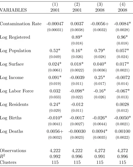
To test the validity of condition (2), we first estimate the correlation between the instrumental variables and the main municipal characteristics that we observe. The results of these estimations are reported in Table5, and show no significant correlation. The fact that we cannot find any character-istic correlated with our instruments is a strong indication that our instruments may not correlated with any unobservable municipal characteristics that impact the budget.
We run a second test that directly addresses the possible correlation between the instruments and municipal finances. We estimate whether either instrument has any significant impact on the
fiscal variables before the elections. First, we test the correlation between our instruments and some fiscal outcomes, for any year before an election year, that is we estimate in OLS the coefficients of the equation:
Yi,y = α log T urnouti+ ωXi,y+ θi,y (8)
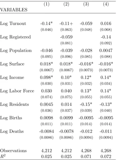
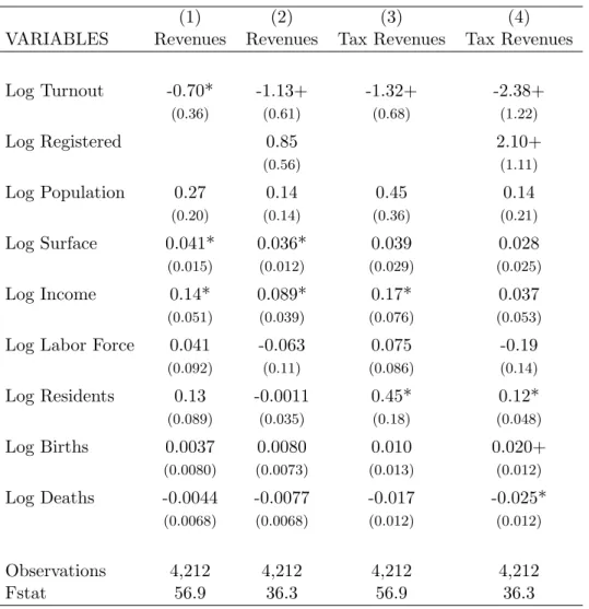
where y < ye, and ye = 2001 or 2008. The results of these placebo tests are reported for municipal revenues in the first two columns of in table6for 2001, and of table7 for 2008. They show no signifi-cant correlation between our instruments and municipal revenues.
Then, we restrict our sample to the observations in the years before an election year ye, and we estimate the effect of the turnout in 2SLS on the change in some fiscal outcome after some arbi-trary year ˜ye < ye in this sample. This amounts to estimating the coefficients of equation5, where ˜ye is a placebo year of elections. The results of these estimations are reported for municipal revenues and some years, in table6for 2001, and in table7for 2008. They show that the instrumented turnout in a year of election ye has no significant impact on the trend in municipal revenues in the years preceding ye.
The previous results thus support the assumption that our instruments are not correlated with factors that may affect some fiscal outcome, or the trend of some fiscal outcome, before the elections.
It is still possible that our instruments affect municipal finances after the elections directly, and not through turnout. For instance, an extremely severe flu epidemics may push a local government to invest in health care infrastructure, to be ready to address future crises. Similarly, terrible weather conditions may force a municipality to renovate its buildings. We have no way to numerically estimate these possibilities. However, the weather conditions, and even the flu epidemics, that we consider, were unusual, but not dramatic. In fact, we couldn’t find in the local newspaper any example of such investment. In addition, investment in health infrastructure is typically decided at a higher administrative level than the municipality22
Finally, we emphasize that all our control variables are observed at least a year before the time of the elections, except the number of registered voters. That number, correlated with turnout, could
22Only very large towns or cities usually invest in significant health infrastructure. Our results hold if we exclude these
thus vary shortly before the elections for the same reason as turnout itself, and bias our estimations. There is indeed evidence that registration records are updated very shortly, or at the time of, the elections. Municipal administration has the possibility to radiate a registered voter up to two months before the elections if it deems that he/she does not reside in the municipality, and radiated voters have the possibility to appeal radiation decisions up to the elections day.23
In addition, we compared the number of registered voters from the two different sources to find that they did not match in a substantial number of cases, suggesting at the very least some measurement error in this variable, likely correlated with the turnout. Given this potential endogeneity of the number of registered voters, we report, for any regression, the results of the estimations with and without that variable.
4
Results
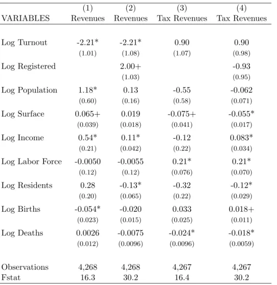
4.1 Effect of turnout on municipal revenues
This section analyzes the effect of turnout on two dimensions of municipal revenues: total rev-enues and tax revrev-enues. For any such variable F , a municipality i, and an election year ye, we define the dependent variable as log Fi,af ter− log Fi,bef ore, where Fi,af ter (resp. Fi,bef ore) is the average of
F over the years of the term starting (resp. ending) in year ye, and ending (resp. starting) in the last (resp. first) year of the term that we can observe.24
In all the regressions, we exclude the specific years of elections 2001 and 2008 because it is impossible to distinguish financial decisions made by the incumbents and by the newly elected council during that year. The specification for these estimations is equation6.
Using this specification, we first report, in Table 8, the OLS estimation of the impact of turnout on total revenues. We find a small effect of turnout on municipal revenues, controlling for municipal characteristics, and this for both elections. These estimations suggest that turnout may have a nega-tive effect on municipal revenues.
The 2SLS estimations are reported in Tables9for the 2001 elections and10for the 2008 elections. They confirm that turnout has indeed a significant negative impact on total revenues, both in 2001 and 2008. The effect is around ten times larger than what the OLS estimation suggested. An increase of 1 percent of turnout decreases municipal revenues by 0.7-2.2 percent, that is an elasticity of around
23The newspaper Ouest France gives the example of a town that radiated almost 10 percent of its registered voters in
2001.
24For the 2001 elections, we thus have: F
i,bef ore ≡ 13
P2000
y=1998Fi,y and Fi,af ter ≡ 16
P2007
y=2002Fi,y, and for the 2008
elections, we have: Fi,bef ore≡ 16
P2007
y=2002Fi,y and Fi,af ter≡12
P2010 y=2009Fi,y
-1.5 on average.
In the other columns of both tables, we show that this decrease in revenues do not necessarily correspond to a decrease in tax revenues, but may stem from a decrease in borrowing, in subsidies re-ceived by the municipality, in use of municipality’s capital, or from a combination of all these sources. However, our data do not allow us so far to distinguish between these sources of revenues.25
In all these regressions, and the following, the coefficient on the log of turnout is roughly the opposite of the coefficient on the log of the number of registered voters, which suggests that it is the percentage of participation, more than the absolute number of voters, that impact the dependent variable. (Again, we stress that these estimations must be interpreted carefully due to the possible endogeneity of the number of registered voters that we discuss in the previous section.)
What is the order of magnitude of these effects? Given that the average budget is 2.02 million and the average population around 1650 inhabitants, a one percent increase in turnout corresponds to a fall in budget around 18 euros per capita per year. We can also express this as the expected impact of an additional vote. Given that the average number of voters who do turn out is around 800, the expected gain for an individual from coming to vote is a decrease (resp. an increase) of around 2.3 euros of yearly budget if he votes for (resp. against) the candidate proposing the lower budget.
These results also provide information on voting costs. We expressed the result as an expected gain or loss in terms of budget for every additional vote, which is in the order of 2.3 euros per year for 6 years (approximately 10 euros in present value for a 0.9 discount factor.26
) If the vote is for a reduction in budget, the maximum welfare gain is easy to express: in the worst case scenario, the voter would not have benefited at all from this extra spending and 910 euros is the maximum expected gain. If the vote is in favor of an increase in budget, it is much harder to interpret since the gain can be larger depending on the utility derived from this expenditure. Furthermore, no information can be obtained for those voters who did not actually turn out.
To go further we therefore need to make some assumptions on the distribution of voting costs. The easiest is to assume that costs are equal across the population. In that case we know, from the previous discussion, the maximum level of financial benefits for voters voting against the increase. Given that costs are identical, we can state that an upper bound on voting costs, net of non financial
25For instance subsidies can be found in several of the categories reported in the summarized accounting data at our
disposal.
benefits of voting such as the satisfaction from achieving a civic duty, is 10 euros.
If voting costs are heterogeneous but are independent of the preferences for the budget, we can also draw conclusions. We could then state that the average voting costs (net of non financial benefits from voting) for the first three quartiles of the population (i.e population that does vote) is below 10 euros. Indeed this can be derived from the behavior of the voters voting against the budget. If this population is identical to those favoring a larger budget in terms of voting costs, we can then draw conclusions for the overall population of voters. We cannot draw any conclusions about those who choose not to vote.
4.2 Effect of turnout on municipal expenses
In this section, we focus on spending variables: total expenses, investment in equipment, personnel expenses, purchases and renovation expenses, and subsidies granted by the municipality. Purchases and renovation expenses are operating expenditures, they comprise expenses to maintain the municipal capital, office stationery, etc. Like in the previous section, the dependent variable is the net increase of the average yearly fiscal variable of interest before and after the elections, and the specification is equation 6.
Tables 11 and 12 report the results of the 2SLS estimation. The largest effect that we find is a decrease in investment in equipment, although it is not significant in 2008. A one percent increase in turnout decreases these expenditures in the order of 3 percent. This category of investments is relatively large. It can correspond to building a school, a road, etc. It can also correspond to the purchase of large electric equipment but does not cover maintenance of existing property.
There is also a negative effect on spending on personnel and small purchases but it is not system-atically significant. The category small purchases corresponds to maintenance and fuels for the city’s vehicles, social events organized by the townhall or transportation cost of municipal staff. The effect is large and significant in 2001. Overall we therefore see that the impact is negative on all categories of spending with a particularly large effect on investments.
4.3 Effect of turnout on electoral outcomes
This section examines the effect of turnout on a selection of electoral outcomes. All regressions are linear probability models based on the specification 6, where the dependent variable is now a probability. Tables13 and 14 report all the results of this section.
Results in Columns (1)-(2) of Tables 13 and 14 show no significant impact of turnout. More impor-tantly, the sign of the coefficient differs from one election to another.
We then estimate the effect of turnout on the probability P2 that the incumbent majority coalition wins a majority of seats in the new council. We find, for both years, a negative impact of turnout.27
Other estimations, not reported here, such as the effect of turnout on the share of seats won by the incumbent majority, give similar results. They all suggest that turnout affects negatively the prob-ability of reelection of incumbent majority members. These estimations are usually not statistically significant.
Finally, we estimate the impact of turnout on the probability P3 that the incumbent majority wins all the seats in the new council - that is the probability that minority is not represented in the council. Overall, more than half municipalities have no presence of minority in the council. We find that the turnout decreases P3, and this effect is significant at 10 percent in 2001.
These results all indicate that higher turnout tends to make the incumbent’s majority more frag-ile and makes it more difficult for him to pass his preferred budget. Several factors make any robust estimation difficult, though, such as the linear probability specification and the 2SLS estimation proce-dure. In addition, the identification of a significant effect of turnout on the strength of the incumbent’s majority is complicated by the nature of the electoral system. For municipalities below 3500 inhabi-tants, individual first-past-the-post voting, gives a lot of flexibility to voters in the composition of the council. Indeed they can pick specifically the name of those they want to vote for without having to vote directly for a list. It is likely that voters, in particular in these small towns, have precise infor-mation about every candidate. Thus, even if the number of seats of each coalition is left unchanged, the identity of the actual councilmen may change, a change we cannot observe with our data and that could further weaken the incumbent coalition.
5
Interpretation of results
Our empirical analysis highlighted two main results. First, an increase in turnout decreases the budget. Second, an increase in turnout decreases the size and strength of the incumbent majority. This result, echoes what has been coined in the political science literature the anti-incumbent effect, i.e the fact that an increase in turnout decreases the probability of reelection of the incumbent, though it
27We cannot define any proper coalition for a substantial number of municipalities, which might lead to a sample
has not been systematically tested.28
We argue that these two results form a coherent story, provided the incumbent promises and implements a higher budget than his or her rival. In fact, we show that this is a natural consequence of a third fact, well documented in the literature and apparently also present in our data, called the “incumbency advantage”.
The “incumbency advantage”, is well established at federal and state levels for the US. For instance Gelman and King 1990 show that the incumbency status translates into about 12 extra percentage points for US congressional elections. Two main explanations for this effect appear to dominate. First, incumbency gives access to resources of different kinds and opportunities to provide community services that facilitate reelection (Mayhew 1974, Fiorina 1977, 1989). Second, there is, by definition, more information on how a candidate could perform in a job he or she has already held.
In our data, the incumbency advantage appears to be present since 65 % of incumbent majority coalitions are reelected. Furthermore, our empirical analysis could suggest a particular source of ”incumbency advantage”, different from the reasons generally mentioned in the literature. It is possible that the incumbent has better access to subsidies or loans for instance. This could suggest that the incumbent has better knowledge of the system or that his previous term allowed him to build political and financial connections.
Regardless of the source of the incumbency advantage, we argue that the three previously dis-cussed facts (incumbency advantage, anti incumbent effect and negative impact of turnout on budget), are mutually consistent in an environment where candidates have preferences for higher budgets.29
Because of the advantage conferred by his status, the incumbent can run a campaign announcing a higher budget than his rival while still maintaining a high probability of obtaining a large majority. In short, the incumbency advantage makes him less accountable. In turn the anti-incumbent effect means that as turnout increases, there is a lower probability that the incumbent obtains a large majority and can pass his budget. Overall the prediction is therefore that higher turnout leads to lower budgets.
In the following section, we develop a model that studies in detail the mechanics of this expla-nation. The main result is to show that the incumbency advantage and anti incumbent effects are simultaneously satisfied under credible assumptions on candidates and voters’ preferences. Note that in the context of our model the anti incumbent effect will correspond to the fact that higher turnout decreases the probability that the incumbent is reelected since we do not want to complicate the
28A notable exception is Hansford and Gomez 2010).
29This seems to be the most common situation that could be due to a variety of reasons: candidates can have some
exposition by explicitly looking at the size of the majority.30
5.1 Model
An incumbent (indexed by I) faces an opposition candidate (indexed by O) in an election involving N voters. The two candidates compete by making binding campaign promises on the budget and its use. All candidates need to provide a minimum level of public goods. They also have pet projects that they can implement at a cost. To simplify the exposition we suppose there are three available choices: C ∈ {L, HI, HO}, where L is the minimum budget, HI is the high budget implementing the
project favored by the incumbent and HO the one implementing the opposition’s favored project.
The incumbency advantage takes a particular form: the incumbent can implement his favored project at a smaller cost than his rival (due for instance to better access to subsidies or to credit). Specifically, denoting bl the minimum budget, the budget required for the opposition to implement
HI or HO is b = bl+ bh while for the incumbent it is only b = bl+ αbh, with α < 1. The parameter
α quantifies the extent of the incumbency advantage (smaller α corresponds to a larger incumbency advantage).
We assume that the preferences of candidates are identical. They get a benefit from being in office r and a benefit B if their preferred project is implemented. Voters have the following preferences: they dislike higher budgets in general but like that their preferred policy is implemented. Specifically, denoting Ci the preferred choice of elector i, preferences are given by −b + G1C=Ci, where b is the
budget implemented by the winner and G is the benefit if the preferred choice is made. We suppose that there are three groups: VI, VN and VOwhere VI is the group of voters who prefer the same project
as the incumbent, VO those who agree with the opposition and VN those who dislike both projects.
We suppose that both groups VO and VI are made up of K < N/2 voters.31
The election is decided by a majority rule. In case of a tie, we break the indifference in favor of the incumbent.32
Because our focus in on turnout, we explicitly model costly voting. Each individual voter faces a cost of voting c which is randomly drawn. If the expected benefit from voting (based among other things on expectations about other voters’ behavior) exceeds the cost, the voter comes to vote. We make the strong assumption that voters in group VI and VO always turn out if their
30Note that we find in our data a negative though non significant effect of turnout on the probability of reelection of
the incumbent.
31We want to maintain the symmetry of the problem and at the same time add no extra advantage for the incumbent
apart from the access to cheaper funding
32Using a different tie breaking rule does not fundamentally change the results but complicates significantly the
preferred project is proposed. Implicitly this is an assumption on the level of G. This simplifies the computation of turnout.
There are two states of the world. With probability p the state is l and the cost of voting is distributed according to F and with probability 1−p the state is h and the cost of voting is distributed according to G, where G first order stochastically dominates F and both distributions have support (0, C). For instance state l can correspond to low incidence of flu and h to high incidence. A move from l to h increases the cost of voting. All voters observe the state before voting but the candidates make their campaign promises under the uncertainty about the state.
5.2 Resolution
We first discuss the equilibrium platforms chosen by the candidates. The incumbency advantage, which is here the fact that the incumbent can fund his preferred project at a cheaper cost, means paradoxically that, in equilibrium, the incumbent will propose a higher budget. Indeed we show that there is no equilibrium where the opposition proposes his preferred project: if both candidates propose their preferred projects, the opposition always loses since the neutral voters of group VN then prefer
the incumbent who has the smaller budget.
As a result only two outcomes turn out to be possible equilibria: (L, L) where both candidates propose the minimum budget and (HI, L) where only the incumbent proposes his preferred project.
At (HI, L), all voters in group VI favorable to the incumbent come and vote. The final outcome
depends on the probability that more than K of the remaining N − K voters decide to turn out (note that given the platform, preferences of voters in VN and VO are perfectly aligned). If bh is low, i.e
the extra budget spent on the non favored project is low, the benefit of voting is minimal and few of these voters will turn out. For a sufficiently low value of bh, the probability that the incumbent wins
will actually be greater than 1/2: guaranteeing the votes of group VI is very valuable. It is then a
dominant strategy to propose HI. On the contrary, if bh is larger, when the incumbent chooses HI
rather than L, he trades off a lower probability of winning against a bigger gain if he does win, since his preferred project will be implemented. Overall this leads to the following result:
Proposition 1. There exists b and r such that:
• if bh< b, the unique equilibrium is (HI, L)
• if bh > b, then if r < B/r, the unique equilibrium is (HI, L) and if B/r < r the unique pure strategy equilibrium (if it exists) is (L, L).
Furthermore r is decreasing in the incumbency advantage α.
Proposition1shows that on average the incumbent will have a higher budget. As the incumbency advantage increases (α smaller), the chances that the incumbent will have a strictly larger budget than his opponent increases. This is intuitive: a larger incumbency advantage means in our contest a lower cost for the pet project and thus lower incentives for the non favored voters to turn out and vote.
We now examine the effect of an increase in turnout on the probability that the incumbent is elected. Specifically we examine a change from state h where voting costs are high (high incidence of flu) to state l. If the equilibrium is (L, L), turnout does not change nor does the probability that the incumbent is elected. The interesting case is when (HI, L) is the equilibrium. In this case, all K voters
in VI turn out while the remaining voters turn out if their cost of voting is low enough, and if they
do, vote for the opposition. Thus a decrease in voting costs increases turnout and since the marginal voters are favorable to the opposition, it decreases the probability that the incumbent is elected. Proposition 2. Moving from state h to l:
1. Weakly increases turnout
2. Weakly decreases the probability that the incumbent is reelected
5.3 Discussion
The model we present exposes a coherent story which, based on a certain type of incumbency advantage, yields both the fact that the incumbent will have a higher budget and the fact that an increase in turnout decreases the probability he is elected. We argue that such a coherent story will naturally emerge, under rather weak conditions, even if the incumbency advantage is modeled differently.
In a companion paper (Godefroy and Henry 2011), we examine an environment where voter preferences are based both on the level of the budget (they dislike higher budgets provided a minimum level of public good is delivered) and on a random preference for one candidate. The candidates on the contrary have a preference for higher budgets. The incumbency advantage means in that paper that the distribution of the taste for one or the other candidate is skewed towards the incumbent. Note that we consider both the case of strategic and non strategic voting and we consider an identical voting cost for all voters.
It is clear, that, as in the model considered in this paper, given his electoral advantage, the in-cumbent will in equilibrium propose a higher budget. The more ambiguous part is to examine whether the anti incumbent effect does hold. We show that this depends on the shape of the distribution of preferences. Consider an increase of voting cost from zero. For a zero cost, all voters vote and the incumbent wins with a probability greater than a half. When the cost increases, if the same number of voters in favor of the incumbent and in favor of the opposition stop turning out, this will have a positive impact on the probability that the incumbent is reelected, since it is a proportionally smaller effect on the number of voters voting in favor. Thus a sufficient condition is that the density of preferences is sufficiently flat.
There are of course other possible interpretations of our results, that we discuss here. The most obvious one is the existence of an exogenous correlation between the individual cost of voting and the preferences for the budget. For instance a lower level of flu could increase turnout only among senior voters, who are more fiscally conservative. Although we have no way of categorically rejecting this explanation, we have several reservations. First, using the two different instruments yields results going in the same direction, and with a similar order of magnitude, though the populations affected may be different. Second, there seems to be no impact of turnout on whether a conservative majority, presumably preferring smaller budgets, is reelected, while the effect on the electoral chances of the incumbent is significant. In addition, the survey based literature that compares voters to non voters, finds that non voters (i.e those who tend not to turnout unless conditions are favorable) tend to prefer higher levels of spending (Leighley and Nagler 2007 for instance). Overall, our model doesn’t invalidate the possible existence of an exogenous correlation between marginal voters and fiscal conservatism, but it shows that negative effect of turnout on municipal budget still holds with weaker assumptions on voters’ preferences.
6
Conclusion
Whereas the focus of most of the literature has been to examine the determinants of turnout, we take in this paper a first step towards understanding the effect of turnout on policy outcomes. We show that higher turnout has a large and significant negative impact on municipal revenues. We use these results to estimate some bounds on voting costs, and we provide an explanation based on a difference between the incumbent and the opposition.
or in flu progression. We cannot categorically claim that our results will systematically generalize to situations where turnout varies for other unanticipated reasons, but we have good reasons to think so. First, the results are remarkably robust, both in sign and in magnitude, regardless of whether we consider the flu or the weather based instruments. Second, the general model we present predicts systematic effects of turnout independent of the source of the variation. Furthermore, other plausible explanations present little consistency with our data.
We conclude by insisting on the fact that we have no way of directly judging whether a decrease in public revenues impacts overall welfare positively or negatively. Regardless of the sign of this impact, however, our paper shows that public policies that are aimed at encouraging voter turnout can have sizable welfare consequences.
Table 1: Summary statistics
Variable Mean Std. Dev. Min. Max. N
Total Revenues 2029.782 14021.286 6.854 1772054.5 57623 Taxes 575.4 3758.66 0 224515.609 57623 Total Expenses 1800.445 13128.751 6.48 1735492.75 57623 Personnel Expenses 479.971 3449.675 -1.017 161546 57623 Purchases 251.609 1314.292 0.926 69103.531 57623 Grants 115.359 1317.416 0 77762.477 57623 Equipment Expenses 459.641 2172.543 -31.199 177904.266 57623 Savings 229.336 1080.597 -3251.291 51769.766 57623 Population 1656.153 6670.265 48 280672 8494 Registered 1137.693 4117.255 29 183511 8537 Turnout 798.653 2326.622 21 101177 8537 Births 19.681 85.861 0 3872 8494 Deaths 13.98 50.370 0 1927 8494
Total Net Taxable Income 14281.854 65653.526 245.414 3600897 8494
Surface 16.571 13.485 0.08 110.28 57623
New Majority Size (/Council Size) 0.867 0.193 0.053 1 8466
Incumbent Maj. Size (/Council Size) 0.597 0.436 0 1 8466
Prob. Majority Wins All Seats (P3) 0.524 0.499 0 1 8182
Contamination Rate -2.445 1.305 -6.279 0.034 8537
Weather Change 0.014 0.023 -0.029 0.064 8537
Table 2: Temperature in 2001/Flu Prevalence in 2008 - Western France
Variable Mean Std. Dev. Min. Max. N
Average Daily Temperature, March 10-11th, 1995-2008 (◦F) 45.733 1.647 42.065 51.003 9168 Daily Temperature, Saturday, March 10th, 2001 (◦F) 53.703 0.901 51.44 55.22 4584 Daily Temperature, Sunday, March 11th, 2001 (◦F) 54.084 1.474 50.54 57.38 4584
Average # Flu Cases per 100,000 Persons, Feb. 9th to March 9th, 1995-2008 790.645 359.635 236.934 1811.378 9168 # Flu Cases per 100,000 Persons, Feb. 9th to March 9th, 2008 1351.604 668.51 2.857 3324.878 4584
NOTES: # Flu Cases is the number of patients with flu-like symptoms reported by a network of general practitioners (see section2.5).
Table 3: Effect of Weather Change on Turnout
Dependent Variable is log Turnout
(1) (2) (3) (4) VARIABLES 2001 2001 2008 2008 Weather -1.34* -0.75* -0.15 -0.054 (0.37) (0.22) (0.14) (0.092) Log Registered 0.89* 0.96* (0.021) (0.018) Log Population 0.53* 0.16* 0.78* 0.058* (0.052) (0.028) (0.033) (0.023) Log Surface 0.026* 0.018* 0.039* 0.016* (0.0058) (0.0025) (0.0040) (0.0021) Log Income 0.089* -0.0047 0.25* -0.012 (0.021) (0.012) (0.021) (0.013)
Log Labor Force 0.032 -0.096* -0.15* -0.064*
(0.028) (0.018) (0.024) (0.012) Log Residents 0.24* -0.0094 -0.0018 (0.031) (0.015) (0.011) Log Births -0.010* -0.0018 -0.025* -0.0046+ (0.0037) (0.0017) (0.0041) (0.0024) Log Deaths 0.0060+ 0.000033 0.010* 0.0012 (0.0031) (0.0019) (0.0036) (0.0022) Observations 4,222 4,222 4,272 4,272 R2 0.992 0.996 0.991 0.996 Clusters 71 71 99 99
NOTES: + Significant at the 10 percent level. ∗ Significant at the 5 percent level. Standard errors are clustered at the meteorological station level.
There is one observation by municipality. Weather change is the net relative increase in temperature between Saturday and Sunday during the elections weekend (Zweain equation 1). Past Weather is the average weather change on the
same days in the previous years. The results with and without the log of the number of registered voters are reported separately due to errors of measurement of this variable possibly correlated with turnout. All regressions include past values of the weather change variable, and regional (departements) and size of municipal council dummies, not reported here.