HAL Id: hal-01081374
https://hal.inria.fr/hal-01081374
Submitted on 7 Nov 2014
HAL is a multi-disciplinary open access
archive for the deposit and dissemination of
sci-entific research documents, whether they are
pub-lished or not. The documents may come from
teaching and research institutions in France or
abroad, or from public or private research centers.
L’archive ouverte pluridisciplinaire HAL, est
destinée au dépôt et à la diffusion de documents
scientifiques de niveau recherche, publiés ou non,
émanant des établissements d’enseignement et de
recherche français ou étrangers, des laboratoires
publics ou privés.
Esma Elghoul, Anne Verroust-Blondet, Mohamed Chaouch
To cite this version:
Esma Elghoul, Anne Verroust-Blondet, Mohamed Chaouch. A Segmentation Transfer Approach for
Rigid Models. Journal of Information Science and Engineering, Academia Sinica, 2015, 31 (3),
pp.993-1009. �hal-01081374�
1
ESMA ELGHOUL*, ANNE VERROUST-BLONDET*AND MOHAMED CHAOUCH+
*Inria Paris-Rocquencourt, Domaine de Voluceau
78153 Le Chesnay Cedex
+CEA List Diasi, CEA Saclay – Nano Innov
91191 Gif sur Yvette Cedex
In this paper, we propose using a segmented example model to perform a semantic oriented segmentation of rigid 3D models of the same class (tables, chairs, etc.). For this, we introduce an alignment method that maps the meaningful parts of the models and we develop a novel approach based on random walks to transfer a consistent segmentation from the example to the target model. The example-driven segmentation is fast and entirely automatic. We demonstrate the effectiveness of our approach through multiple results of inter-shape segmentation transfer presented for different classes of rigid models.
Keywords: segmentation transfer, 3D alignment, Random walks, graph partitioning
1. INTRODUCTION
Mesh segmentation partitions the surface into a set of patches under some criteria. Comparative studies and surveys on segmentation techniques [1, 23, 8, 2] clearly distinguish between geometric and semantic-oriented approaches. We are interested here in retaining the semantic information during the segmentation. Our aim is to address the challenging task of automatically identifying the semantically meaningful parts of a 3D model, which can be hard to achieve when only the shape geometry is considered. We propose a novel segmentation transfer approach for rigid mod-els. The user provides the desired semantic information by segmenting one model into meaningful parts. Then, given this model as an example, a similar segmentation is carried out on each model of the same class.
Achieving meaningful segmentations of single shapes by exploring geometric properties of the mesh is in continuous progress. Recent works include the use of heat walk [3], minimum slice pe-rimeter [12] and intrinsic primitive decomposition [28]. To overcome the limitations related to the low-level geometric segmentations of single shapes, researches have turned to partitioning the surfaces of a family of models in a similar way [11-14, 20, 22, 24, 26, 27]. Their goal may be slightly different from ours, as in most cases it is restricted to obtaining consistent mesh partitions. In [14, 20, 22, 24, 26] the meshes are divided into parts that may be non-connected (group the four legs of chairs in one region of the surface, for example), which is not what we want to achieve. The unsupervised technique of Huang et al. [13] jointly segment shapes using linear programming. This approach works well for non-rigid models as it is robust to shape variations but it does not guarantee a consistent segmentation of an entire set. Likewise, the skeleton based approaches of [9, 31] work better on articulated models as they map a segmentation of a source mesh to a target mesh based on the skeleton correspondence between meshes. On the other hand, the co-segmentation method of [11] is extended to a technique that transfers a segmentation from an example to a set of models. They base their approach on a rigid alignment of shapes and resolve a graph clustering problem in order to compute an unsupervised co-segmentation of a set of shapes. We differ from their work in that we perform a model-to-model segmentation that is rapid and parameter-free.
2 Our approach is based on two key hypotheses.
[H1] First we assume that the example segmentation decomposes the model into meaningful parts that could be identically produced by a random walk segmentation algorithm [19], i.e., these parts could have been computed from a set of pseudo seeds appropriately chosen on the 3D mesh. The choice of the random walk algorithm was motivated by the evaluation results of [8], which show that the random walk method outperforms the K-means approach [25] in producing close-to-human segmentations.
[H2] If we focus our attention on rigid models, we can notice that the models belonging to the same class can be consistently aligned in order to obtain a similar organization of their meaningful parts. For example, any chair has a natural decomposition into the following parts: a “back”, a “seat” and its “legs”. These parts are respectively located at the top, in the middle and at the bot-tom, when the chair is in an upright position. Moreover, when two chairs are aligned together, the locations of their corresponding parts may differ only by a small local translation, a local rotation or difference in size.
As our objective is to reproduce the desired segmentation on the target model, a flexible mentation process is necessary. Thus, we develop a derived approach from the random walk seg-mentation method [19] and transform the problem of segseg-mentation transfer into a problem of lo-cating seed faces on the target model, given the pre-segmented example model. To perform this localization we introduce a method that aligns each model of the same class w.r.t. the example model.
2. METHOD OVERVIEW
In what follows, �� will denote the segmented model given as example, with ��1..��� its N segments, C its class of models and �� any model of C. The segments that will be computed for �� are denoted by ��1..���, where ��� is associated with the segment ���. All the models are
tri-angulated 2-manifold meshes.
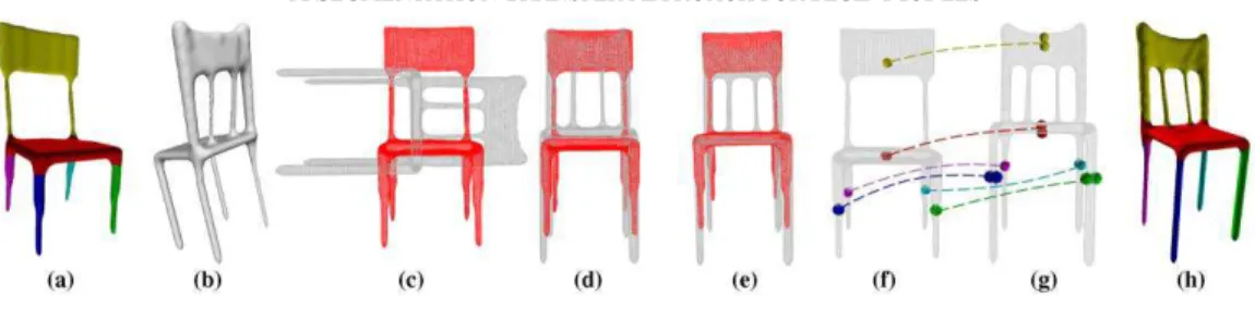
Our segmentation transfer method consists of the following steps, which are summarized in Figure 1:
- First of all, each mesh �� of C is aligned with �� in such a way that the distances between the main parts of �� and �� are minimized.
- In a second stage, a rough localization of �� pseudo seeds and a seed placement strategy on �� is performed. In order to avoid some errors related to the model meshing, several seeds per
segments are introduced. The basic random walk algorithm [19], which computes the resulting segmentation of ��, has been extended for this purpose.
Our contributions are the following:
• A straightforward method to align one object to another from the same class is presented. The method associates the functional parts of the two 3D models.
• A robust and automatic seed localization algorithm is described. The set of localized seeds, when used as input to the random walk method, results in a meaningful segmentation of the target mod-el. In addition, this algorithm yields the correct matching of the computed segments with the ex-ample model segments.
• An extension of the random walk method accepting more than one seed per segment as input is proposed. Consequent improvements are studied. In particular, we show that it resolves many problems due to the model shape and meshing.
• An original boundary smoothing process constrained by the adjacencies of the segments of ��.
The organization of this paper is as follows: Section 3 describes the multi-seed random walk algo-rithm used in the second step; Section 4 details the three steps of our alignment process; Section 5 presents the seed placement strategy and the segmentation of the target model; improvements achieved by the multi-seed per segment approach and segmentation transfer results are presented in Section 6.
3
Fig. 1. The whole segmentation process. (a): the segmented example model��; (b): the target model ��; (c), (d) and (e): the three steps of the alignment process; (f): localization of pseudo seeds on ��; (g):
multi-ple seeds on �� and (h): resulting segmentation on ��.
3. MULTI-SEED RANDOM WALK SEGMENTATION METHOD
The random walk mesh segmentation method introduced in [19] builds segmentations of any 2-manifold triangulated model M. It splits M into N meaningful pieces using N faces �1...�� of M given as seeds. The segmentation is computed by assigning a value i, i = 1, ..,N to each non-seed face ��, l = 1, ..,m of M, where i is the index of the seed face �� that has the highest probability ��(�
�) of being reached first by a random walk from �� on the dual graph of M, i.e.,
��(�
�)>��(��) for � ≠ �. Probabilities �� introduced in [19] lead to the creation of segment
boundaries on edges of high negative curvature and ensure that each segment is a contiguous re-gion of the surface. They satisfy:
� ��(� � ) =∑3�=1��,������,��, � = 1, … , � ��(� �) = 1 ��(� �) = 0 when � ≠ �
(1) where ��,�, j =1..3 are the three faces adjacent to �� and ��,� are crossing probabilities computed following [19]:
��,�=�����,����� �−����� ,��,��
��
���� � (2)
with �� such that ��,1+��,2+��,3= 1, ���,�� is the length of the edge common to �� and ��,� , and �� is based on the dihedral angle measure between faces �� and ��,�:
�����,��,�� = � �1 − cos ���ℎ��������,��,���� (3)
� gives priority to the concave edges: � = 1 for concave edges and � = 0.1 for convex edges. �� is normalized by the average over all edges ����. �
Let �� be the vector of the m probabilities ��(��), for i = 1, .., N. As explained in [19], the problem can be written in matrix form through N independent linear systems:
�����= �� (4)
Each row of ��� contains at most four non-zero values and �� has at most three non-zero values, corresponding to the three faces adjacent to the seed face ��. The N linear systems form a sparse system, which makes the fast computation of the ��(��) possible and allows the segmenta-tion of M to be done within a reasonable time.
This overall scheme is extended here to accept multiple seeds per segment. Its use for segmen-tation transfer will be discussed later. Consider the case of doubling the number of seed faces to
4
obtain the same number of segments N in the final result. We start by assigning the same index i to two different seed faces ��1 and ��2 for each i = 1,2, ..,N. While the number of non-seed faces is reduced by N (m′ = m − N), the number of random walk probabilities to be computed for a non seed face �� stays unchanged and equals N. In fact, instead of computing the probability that a random walk starting at �� first reaches one seed face from the set provided, we compute the probability that this random walk first reaches any of the two seed faces ��1 and ��2 to decide if �� belongs to the region indexed by i. The probabilities of seed faces are now defined as:
� ������� = 1 ��� � ∈ {1,2}
����
��� = 0 ��� � ∈ {1,2} ��� � ≠ �
(5) A slight modification to the linear system of Equation (4) enables us to describe the multi-seed approach by N linear systems of the form:
��′×�′��= �′� (6)
Note that the size of ��′×�′ is inferior here and that ��′×�′ always has four non-zero values by row at most. The number of zeros also decreases in �′� because �′� can contain up to six non-zero values corresponding to the faces adjacent to ��1 or to ��2.
The process can be adapted to hold an arbitrary number of seed faces per segment when neces-sary. Nevertheless, as the complexity of a sparse system is also proportional to the number of non-zero elements, the overall number of seeds should be limited to avoid a significant slow-down of the segmentation process. Moreover, particular attention should be paid to the placement of the additional seeds. It is indeed not guaranteed that each region produced by the multi-seed segmen-tation process is connected. A strategy for the placement of two seeds on a region surface is de-scribed in Section 5.2.
4. ALIGNMENT PROCESS
The input to our algorithm is a pair of arbitrary oriented 3D meshes, �� and ��, belonging to the same class C of models and representing the example and the target models respectively. The alignment process is performed in three steps.
We first calculate three orthogonal alignment axes, following [7], for each model: this method computes three axes that consistently align the 3D objects within the same semantic class of mod-els and obtains good results on rigid modmod-els. These axes are given in arbitrary order and orienta-tion. Thus, for each model, 48 coordinate systems can be built by performing permutations and inversions of the axes. This number can be reduced to 24 if we consider only direct orthonormal systems.
5
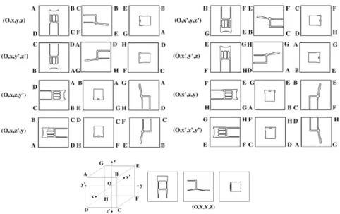
Fig. 2. Top to bottom: 8 triplets of silhouette images built from the projection of �� on the unit cube faces, with their corresponding candidate coordinate systems and, in the last row, the silhouettes built from the pro-jection of �� on the three faces orthogonal to �������⃗, �������⃗ and �������⃗. Here the triplet (�, �,�, �) aligns the best
�� and ��.
The second step consists in fixing the orientations and the order of the alignment axes. To avoid comparing the 3D meshes, we normalize the models to their axis aligned unit cubes and use these cube faces, considering that the two models are correctly aligned when the silhouette images of their projections on the cube faces are similar. For each model, the silhouette images on the cube faces correspond to, at most, three different shapes, up to a rotation (a quarter, half or three quarter turn) and/or a flip. In order to compare the appropriate faces, we choose a direct orthonormal ref-erence system(�, �, �, �), where �������⃗ = �������⃗˄�������⃗ and compute the projections of �� on the three faces orthogonal to �������⃗, �������⃗ and �������⃗ (see Figure 2). From the canonical unit cube of ��, we compute eight sets of three silhouette images corresponding to the projections of �� on the faces associated to the eight candidate orthonormal systems (�, �, �, �) , (�, �, �′, �′),(�, �, �, �′),(�, �, �′, �), (�, �′, �, �′) , (�, �′, �′, �) , (�, �′, �, �) and (�, �′, �′, �). Each set of three silhouette images is associated to three triplets obtained by a circular permutation of the oriented axes, i.e. (�, �, �, �), (�, �, �, �) and (�, �, �, �) for the first set of images in Figure 2. Then, 24 triplets of silhouette images corresponding to the 24 candidate reference sys-tems for �� are compared with the triplets of silhouette images built from ��. The contours of the silhouettes are extracted and a rigid ICP algorithm compares the fixed alignment provided by the three contour images of �� with the 24 triplets of contour images of ��. The triplet of con-tours that has the minimum ICP error defines the ordering and the orientation of the axes that best align �� to ��. At the end of this stage, �� and �� are aligned together.
A closer alignment of �� w.r.t. �� is needed in order to establish correct matchings between the segments of �� and parts of ��. This is done during the last step of the alignment process. Our goal here is different from [16, 21] where the purpose is to find the best rotation to align glob-ally two models together. As we want to align the main parts of �� and ��, this step may in-volve both translations and rotations: our refinement consists in applying to �� a rigid transfor-mation computed through a global 3D ICP algorithm [4] performed on �� and �� together. Since the two models are already globally aligned, the use of such an approach is suitable. At the
6
end of this process, the main parts of �� and �� are accurately aligned and the two models are defined in a common coordinate system R.
One should note that this alignment process could have been replaced by the extrinsic align-ment of Kim et al. (step 3a of [17]): it would generally give similar alignalign-ment results and the two methods have a similar complexity. Nevertheless, our two first steps compute the reference frames that align consistently a set of rigid models belonging to a same class of models and can be used alone for this purpose.
5. SEED LOCALIZATION STRATEGY AND SEGMENTATION OF M
TWe now need to define an appropriate set of seed faces on �� in order to use the random walk approach to transfer the segmentation of �� on ��. As the segments of �� and the parts of �� corresponding to them are close in space, the computation of the seed faces on �� uses a
rough localization of seed faces associated to the segments of �� . The cuts obtained by the ran-dom walk segmentation are refined in a last step using a graph cut algorithm.
5.1 Localization of ME Pseudo Seeds
The segmentation given for �� provides a decomposition of �� into meaningful parts. Thus, using hypothesis [H1], a similar segmentation can be performed on �� by the random walk method, with an appropriate set of seed faces of �� . As we don’t want to compute them here, we denote them pseudo seeds. The random walk algorithm is robust with respect to the location of the seeds and creates segment boundaries around edges of high negative curvature. However we should avoid estimating the pseudo seed locations near the segment borders, which are often of high concavity. The central region of the segment is therefore a more appropriate position for pseudo seeds. Let �� be the centroid, with respect to Euclidean distance, of the subpart of �� corresponding to segment ���. The point �� gives a rough estimation of the pseudo seed
loca-tion of ���: the set of mesh faces belonging to ��� and close to �� should contain the pseudo seed of ���.
5.2 Seed Placement Strategy on MT
In order to transfer the segmentation of the model �� onto the unsegmented model ��, one intuitive approach is to select the face of �� closest to the centroid �� of ��� as the seed face for the region corresponding to the segment ��� and use random walks to segment ��. Although seed-based algorithms are traditionally initialized with one seed per surface region, such a mono-seed approach may fail to detect boundaries that are not clearly defined. Moreover, the ran-dom walk method may lead to an incorrect segment if the seed face belongs to a concave region. Thus we extend the initialization of the segmentation algorithm by setting a couple of seeds per segment instead of a singleton, as input to the random walk algorithm. The first seed face ��1of ��� is assigned to the face of �� that is closest to the centroid �� of ���, where �(��,�) is the
Euclidean distance between �� and the centroid of a face f of the polygonal mesh of ��:
7
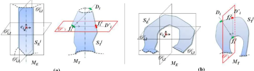
Fig. 3. Seed placement strategy on ��: (a) The plane Pi,2 is computed using ���. In ��, D′i is the projection
of Di on P’i (plane parallel to Pi,2 and containing the center of ��1). D′i encounters the mesh surface on the
second seed face ��2. (b) Both planes Pi,1 and Pi,2 do not intersect the boundary edges of ���. However only Pi,1
splits the surface region in two parts separating the closed boundaries across two different sides which makes it more suitable than Pi,2 for the placement of ��2, thus P’i is parallel to Pi,1.
While the localization of the first seed face is straightforward, the selection of the second one requires more attention. An incorrect selection of the second seed may directly affect the segment connectivity property, ensured a priori by the use of a single seed per segment. To overcome this problem, we use local principal planes computed from ���. to guide the placement of the second seed face. These planes are defined through a continuous principle component analysis (CPCA) [29] performed on the example segment ���. In fact, the CPCA appears to be more complete and the most stable of all the PCA-approaches we have studied. It computes three orthogonal eigen-vectors of the covariance matrix for the surface part of ���, working with sums of integrals over mesh triangles instead of sums over vertices [29]. The local alignment of ��� is thus provided through three local principal vectors �������⃗, ��,1 ������⃗ and ��,2 ������⃗. Note that the example segment ��,3 �� and its corresponding target segment on �� are assumed to have almost the same pose in the global model alignment. Thus, we expect the local principal vectors of ��� to be close to those computed for ���. The local principal plane used for the localization of the second seed ��2 of ��� is denoted by Pi and is the one of the 3 candidate planes (i) which contains ��, (ii) normal to one of the
vec-tors �������⃗ (�,� Pi,k = (��, �������⃗ ) with k = 1..3) and (iii) not intersecting the set of edges composing the �,�
boundaries of ���, if it exists. When more than one plane satisfies (i), (ii) and (iii), we give priority to the one which splits ��� in two parts separating the distinct closed boundaries (Pi,1 in Figure
3(b)). When none of the three planes satisfies the three given conditions, we keep only one seed for this segment.
The role of Pi is to guide the localization of the second seed ��2 to ensure that it will remain
near the central zone of the target segment region and far from its boundaries. The second seed face ��2 is chosen from the faces of �� that intersect the plane P’i, parallel to Pi and containing
the centroid of ��1 as follows: an oriented half line Di from the centroid of the first seed face ��1,
directed by the inward-pointing normal to ��1 is computed. This half line is projected on P’i into an
oriented half line D′i. The second seed ��2 corresponds to the face of �� that first intersects D′i
(see Figure 3). The first intersection of D′i with �� encounters a face that normally belongs to the
same part of the model, but opposite ��1. Setting a couple of seeds per segment implies that we assign the same segment label to two seed faces in the initialization stage. Thus we use the mul-ti-seed random walk segmentation method described in Section 3 to perform the segmentation of ��, with 2N seed faces ��1 and ��2, 1 ≤ i ≤ N.
8 5.3 Boundary smoothing
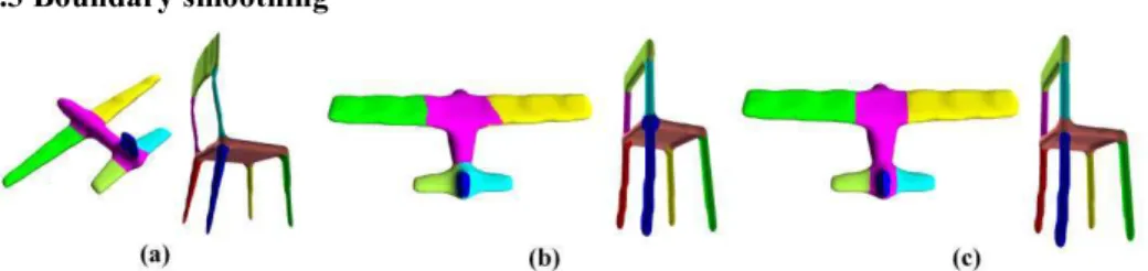
Fig. 4. Boundary smoothing: (a) two example models, (b) their two respective target segmentations using the multi-seed random walk algorithm and (c) boundary smoothing and correction of segment adjacency
graph using the graph cut algorithm with non uniform interaction potentials.
Sometimes the boundaries of the computed segments may need a refinement step in order to ad-here to the natural contours of the shape parts. Thus we introduced a second partitioning algorithm that uses the alpha-beta swap (α-β swap) algorithm for graph cuts of Boykov et al. [6]. In fact, this method improves our previous approach in two ways: it smooths the segments boundaries and it also enforces the boundary creation between segments whose corresponding segments in ME are
adjacent. The algorithm minimizes an energy function E(L) over the mesh MT, taking into account
the probabilities computed by the random walk algorithm, the boundaries between adjacent seg-ments of MT and the adjacency graph ��� built from the segments of ME. The new labeling L,
computed with the α-β swap algorithm, assigns a segment label Lfϵ {1,..,N} to each face f of MT
such that all the cuts between these newly computed segments are refined. Let Na be the set of
pairs (f, g) of adjacent faces of MT. E(L) is composed of a data energy Ed(L) and a smoothness
en-ergy Es(L), E(L) =λ Ed(L)+ Es(L) with:
��(�) = ∑� ���� �� ��− �������(�) + ��, ��(�) = ∑(�,�) ������(�, �). �(��,��) (8)
where λ is a weighting parameter (here λ = 0.2 to give higher priority to Es(L)), the values ���(�)
are derived from the probabilities computed by the random walk algorithm and the capacity func-tion cap(f, g) is defined on the arc that links adjacent faces f and g as in [15] to enforce the creafunc-tion of segment boundaries through concave short edges. The interaction potential V is a semi-metric used to penalize pairs of different labels (Lf , Lg) = (j, k),with j≠ k:
�(�, �) = �
1 �� �����,���� = ����,����
�1 > 1 �� �����,���� = 1 ��� ����,���� = 0 �2 < 1 �� �����,���� = 0 ��� ����,���� = 1
(9)
where A(S, S’) = 1 when the two segments S and S’ are distinct and adjacent, and A(S, S’) = 0 in the other cases. If j=k, then V(j,k) = 0. Note that the value u1 heavily penalizes the cut between
segments that are adjacent in the random walk segmentation ST while their corresponding
seg-ments are not adjacent in ME and the value u2 favors the boundary creation of a cut between
dis-connected segments of ST corresponding to adjacent segment in ME. We obtained good
segmenta-tion results on the evaluated model sets with u1 = 5 and u2 = 1/5. This process improves the
quali-ty of the boundaries and rectifies, whenever possible, incoherent segment adjacencies as illustrated in Figure 4.
9
6. EXPERIMENTS AND RESULTS
We evaluated our example-based segmentation on man-made objects extracted from two da-tasets. The method was tested on the whole sets of irons and goblets from the COSEG Dataset [30] by using each provided ground-truth segmentation as an example for all the class meshes. We also chose three rigid categories (chairs, airplanes and tables) from the Princeton Segmentation Benchmark [8]. In each category, the human segmentations are not consistent and present slightly different styles and numbers of segments. Thus, we fixed the number of segments and the style that is the most typical in the category. Then for each model, we selected one ground-truth seg-mentation from the benchmark that possesses the chosen style and number of segments. If that style did not exist in the data provided, we created it manually for the model. We also adjusted the segment indexes manually to obtain the segmentation consistency needed for our tests. When ap-plying the multi-seed and the mono-seed approaches, each model took the role of the example �� once for all the models of its class. Figure 7 show some segmentation transfer results using our
approach for different classes of models. For the chair sets, different example models are shown with various styles of exemplar segmentation.
Fig. 5. Improvements of segmentation transfer results through the multi-seed approach (before boundary smoothing): (a) the airplane model used to segment the models in (b), (c) and (d); (b) mono-seed
segmenta-tion of a target airplane, computed posisegmenta-tions of seeds are shown on two opposing views of the model; (d) segmentation transfer using couples of seeds and better detection of the wing borders; (c) from left to right :
mono-seed, double-seed without planes Pi and double-seed using planes Pi; (e) and (f) left: ��, right: im-provements produced on the multi-seed segmentation of �� in comparison to its mono-seed segmentation.
The Recognition Rate scores, as defined in [14], are reported for the different categories in Fig-ure 6. The measFig-ure gives the percentage of identically labeled surface area of the mesh across two segmentations of the same model: the segmentation created by transfer and the ground-truth. The histogram shows that the multi-seed approach outperforms the mono-seed approach on all the test data. Table 1 reports segmentation errors using the evaluation metrics proposed in [8]. The Cut Discrepancy considers boundary matching by measuring the distance between matching cuts, whereas the Rand Index compares pairwise label relationships in two segmentations. Again, the multi-seed segmentation obtains better results than the mono-seed one.
10
Fig. 6. Comparison between the multi-seed approach after boundary smoothing and the mono-seed approach through Recognition Rate scores evaluated for different classes of rigid 3D models.
Multi-seed VS mono-seed results. Let us first comment on the examples presented in Figure 5. For models (b) and (e), the geometric information about concavities varies considerably and can be very poor. This leads to incorrect propagation of the segmentation if a single seed defines the seg-ment. For the wings of the airplane in (b), segmented by the model in (a) with a mono-seed ap-proach, the seed locations are unfavorable and only the side near strong concavities is detected. The other flat side is mixed up with the neighboring central segment with which the wings share unclear long borders. Positioning opposing seeds near less concave borders of the wings consider-ably improves the segmentation result. It also fixes the matchings between the segmented parts of the target and the example models. Other cases of better border detection with the double-seed approach are shown for the “back” segment of the chair in (e) and the upper segment of the goblet in (f). The airplane in (c), segmented by the model in (a), shows in its rightmost segmentation how the use of locally computed planes Pi helps to guide the positioning of the second seed inside the
region surface, compared to the middle segmentation where these planes were not used.
Table 1. Comparison of the mono-seed and the multi-seed created segmentations (with the boundary smoothing process) according to the ground-truth co-segmentation. Chair 6S (resp., Chair 8S) corresponds to
a 6 segment (resp., 8 segment) ground-truth for chairs.
Rand Index Cut Discrepancy MultiS MonoS MultiS MonoS
Chair 8S 3.3 3.5 9.2 13.8 Chair 6S 6.9 8.9 18.0 20.3 Goblet 12.3 18.0 21.2 56.1 Airplane 7.3 19.2 8.8 21.6 Iron 16.5 21.5 15.9 22.0 Table 8.4 13.5 17.0 22.3
Comparison to related work. A comparison to individual segmentation methods is provided in Figure 8. The Rand Index is computed this time against all human generated segmentations of the Princeton Benchmark [8] for the classes concerned. We show the scores of the random walk method of Lai et al. [19], the shape diameter [24] and the randomized cuts [10], the leading meth-od on the benchmark [8]. We achieve better scores than all the segmentations evaluated in [8]. We can deduce that the use of an example model to create consistent segmentations improves the par-titioning of the shape and consequently the individual segmentation result. Moreover, on rigid models our Rand Index scores are similar to the supervised approach of Kalogerakis et al. [14] with 3 training models and to the unsupervised approach of Huang et al. [13] in the JointAll condi-tion in which they obtained their better scores.
11
Fig. 7. Segmentation by transfer presented for a variety of example models. �� is always on the left of the line and segmented target models are on the right. Our method produces good results, even when changing
the segmentation styles and �� as shown for the sets of chairs.
To perform a direct comparison with the supervised approach of Kalogerakis et al. [14], we as-sociated the same labels to all similar part types in our example segmentations (i.e. one label for the four legs of the chair models) and performed a segmentation transfer for three classes of the benchmark [8] (20 segmentations for each model). Table 2 shows the Recognition Rate scores obtained by our approach with these exemplar models and those obtained by the learning method of Kalogerakis et al. [14], with three models per training set. The performances of the two ap-proaches on these classes of models are very close. Note that in [14], the more training models are added, the better the results are. Therefore, such supervised approach would be advantageous for large sets of shapes and less adapted to smaller sets, for which our method proved to be effective and more efficient.
Table 2. Recognition Rate scores on 3 classes. Comparison with the supervised approach of Kalogerakis et al.: SB3 corresponds to the scores of Table 1 in [14] with 3 models used as training set.
Recognition Rate Chair Airplane Table Average SB3 [14] 97.1 91.2 99.0 95.7 MultiS 96.2 92.8 91.7 93.5
12
Let us examine the segmentation results on the chairs in Figure 7. The segmented example of the second row corresponds to one of the four chairs belonging to the learniing set of Kalogerakis’ method in Figure 3 of [14]. We see that the segments created by our approach on the same target models resemble those of Kalogerakis et al. (chairs (a) in Figure 3 of [14]) and are visually better than those obtained by Golowinskiy and Funkhouser’s method [11] (chairs (c) in Figure 3 of [14]), where the boundaries are not always correctly detected.
The last row of Figure 7 shows that our method can work on sets of objects that have very sim-ilar shapes and parts, as airplanes and birds, even though they do not belong to the same class of models.
Validation of [H1] hypothesis. We consider here the segmentation built on each model using its own ground truth segmentation. The average Recognition Rate score obtained over the three eval-uated rigid classes (60 models) is 96.45%. This high score confirms that a random walk segmenta-tion algorithm can compute segmentasegmenta-tions similar to the meaningful exemplar ones, as assumed in [H1] in section 1. This result also validates our seed placement strategy.
Fig. 8. Rand Index scores. MultiS corresponds to our method. Ex, SB3 and JointAll correspond respectively to our exemplar pre-segmented models, the supervised approach of Kalogerakis et al. [14] with 3 training models and the unsupervised approach of Huang et al. [13]. Lower values of the Rand Index indicate better
similarity to human-generated ground truth.
Performance. It was previously demonstrated in [8] and [19] that the interactive response time is the greatest benefit of the random walk segmentation method. As for our approach, the whole pro-cess usually took less than one minute for a couple of arbitrary oriented input models composed of less than 20K triangles. The experiments were carried out on an Intel Core i7 2.8GHz PC. The running time of the alignment step took a few seconds, equivalently to the second and the last steps of computing a consistent segmentation. The approximate complexity of the linear sparse system is O(m′N), with m′ the number of non-seed faces and N the number of segments. We used a c++ iterative solver for sparse systems of linear equations to compute the random walk probabili-ties. For the α-β swap algorithm, we used the implementation provided by [6, 8, 5]. Default values of control parameters involved in probability computation, convergence error and the α-β swap algorithm were set once for all the experiments. We conclude that our approach is parameter-free as it depends only on the exemplar model, and it achieves the best running time compared with existing approaches, e.g., the required off-line training process on pre-labeled models in [14] may take hours and their on-line segmentation of one mesh may take some minutes.
13
Extension of the method. In order to make segmentation transfer more flexible, a number of in-teractive tools are proposed to the user: he can insert or delete segments and design the style of the desired exemplar segmentation by combining existing styles.
Fig. 9. A combined use of two different style exemplar segmentations (middle) to obtain the desired result on the target model (right).
For instance, it is not possible to create a meaningful partitioning of the four-legged chair on the left of Figure 9 using the one-legged example chair alone. Also it is useless to have this chair’s “back” decomposed into three regions as in the middle four-legged model. A user-defined combi-nation between the two exemplar segmentations is possible as the overlapping indexes correspond to semantically similar parts (e.g., the green “seat” for these chairs). This leads to a more con-sistent segmentation for the target model, as shown on the right of Figure 9.
Limitations. As our method is based on alignment hypothesis, the use of a good alignment process is of great importance in order to get a good initial seeding of the target regions. Moreover, when a class presents large shape variability, such as the vase class of Figure 7, it may be insufficient to use only one model to consistently segment the others.
On the other hand, our method, in its automatic version, always computes the same number of segments as in the example and doesn’t detect outliers segments on models (see the rightmost table segmentations in Figure 7 for example). To deal with these issues, we can use the symmetries of the input shapes, since the design of man-made objects is commonly based on symmetry attributes. A possible approach would be to capture the symmetries of the example and target models in order to compare them, after processing the alignment step and before positioning seeds. These symme-tries can be reflective, rotational or translational along a direction. Also they can be examined lo-cally or globally. Inconsistent segments can be avoided by detecting their absence on �� and eliminating their corresponding seeds. Likewise, extra parts of �� can be identified and addition-al seeds can be created for them by symmetry. We addition-also believe that such an approach may dramat-ically reduce errors due to intra-class geometric variabilities.
This method is not adapted to non-rigid models as our hypothesis [H2] cannot always be satis-fied: the objects may present a large variability in shape inside a same class of models. Thus the skeleton-based approaches [9, 31] are more appropriate in this case.
7. CONCLUSION
We have presented a fast and efficient method that takes a segmented rigid model and transfers meaningful and consistent segmentations on unsegmented models from the same class. The algo-rithm produces individual segmentations that are more meaningful and improves upon techniques that segment objects separately. In addition, as the approach is fairly fast, it is particularly well-suited to addressing the needs of interactive applications. Experiments conducted on various sets of rigid models showed the effectiveness of our segmentation transfer approach and the soundness of our two key hypotheses [H1] and [H2] presented in section 1.
14
REFERENCES
1. M. Attene, S. Katz, M. Mortara, G. Patanè, M. Spagnuolo, A. Tal, “Mesh segmentation - a comparative study,” in Shape Modeling International, 2006, p. 7.
2. H. Benhabiles, J.-P. Vandeborre, G. Lavoué, M. Daoudi, “A framework for the objective evaluation of segmentation algorithms using a ground-truth of human segmented 3D-models,” in Shape Modeling International, 2009, pp. 36-43.
3. W. Benjamin, A.W. Polk, S. Vishwanathan, K. Ramani, “Heat walk: robust salient segmenta-tion of non-rigid shapes,” Computer Graphics Forum, Vol. 30, 2011, pp. 2097-2106.
4. P.J. Besl, N.D. McKay, “A method for registration of 3-D shapes,” IEEE Transactions on Pattern Analysis and Machine Intelligence (IEEE TPAMI), Vol. 14, 1992, pp. 239-256. 5. Y. Boykov, V. Kolmogorov, “An Experimental Comparison of Min-Cut/Max-Flow Algorithms
for Energy Minimization in Vision,” IEEE TPAMI, Vol. 26(9), 2004, pp.1124-1137.
6. Y. Boykov, O. Veksler, R. Zabih. “Fast approximate energy minimization via graph cuts,” IEEE TPAMI, Vol. 23(11), 2001, pp.1222–1239.
7. M. Chaouch, A. Verroust-Blondet, “Alignment of 3D models,” Graphical Models, Vol. 71, 2009, pp. 63–76.
8. X. Chen, A. Golovinskiy, T.A. Funkhouser, “A benchmark for 3D mesh segmentation,” ACM Transactions on Graphics, 2009, 28(3).
9. E. Elghoul, A. Verroust-Blondet. “A Segmentation Transfer Method for Artic lated Models,” in Eurographics (Short Papers), 2013, pp. 17–20.
10. A. Golovinskiy, T. Funkhouser, “Randomized cuts for 3D mesh analysis,” ACM Transactions on Graphics (Proc. SIGGRAPH ASIA), Vol. 27, 2008.
11. A. Golovinskiy, T.A. Funkhouser, “Consistent segmentation of 3D models,” Computers & Graphics, Vol 33, 2009, pp. 262-269.
12. T-C. Ho, J-H. Chuang, “Volume based mesh segmentation,” Journal of Information Science and Engineering, Vol. 28, 2012, pp. 705-722.
13. Q.X. Huang, V. Koltun, L.J. Guibas, “Joint shape segmentation with linear programming,” ACM Transactions on Graphics, Vol. 30, 2011.
14. E. Kalogerakis, A. Hertzmann, K. Singh, “Learning 3D Mesh Segmentation and Labeling,” ACM Transactions on Graphics, Vol. 29, 2010.
15. S. Katz, G. Leifman, A. Tal, “Mesh segmentation using feature point and core extraction,” The Visual Computer, Vol. 21, 2005, pp.649-658.
16. M. Kazhdan, “An approximate and efficient method for optimal rotation alignment of 3D models,” IEEE TPAMI, Vol. 29, 2007, pp. 1221-1229.
17. V.G. Kim, W. Li, N. Mitra, S. DiVerdi, T. Funkhouser, “Exploring collections of 3D models using fuzzy correspondences,” Transactions on Graphics (Proc. of SIGGRAPH 2012), Vol. 31, 2012.
18. V. Kolmogorov, R. Zabih, “What Energy Functions can be Minimized via Graph Cut,” IEEE TPAMI, Vol. 26(2), 2004, pp.147-159.
19. Y.K. Lai, S.M. Hu, R.R. Martin, P.L. Rosin, “Rapid and effective segmentation of 3D models using random walks,” Computer Aided Geometric Design, Vol. 26, 2009, pp. 665-679. 20. P. Luo, Z. Wu, C. Xia, L. Feng, T. Ma, “Co-segmentation of 3D shapes via multi-view
spec-tral clustering,” The Visual Computer, Vol. 29, 2013, pp. 587-597.
21. M. Martinek, R. Grosso, “Optimal rotation alignment of 3D objects using a GPU-based simi-larity function,” Computers & Graphics, Vol. 33, 2009, pp. 291-298.
22. M. Meng, J. Xia, J. Luo, Y. He, “Unsupervised co-segmentation for 3d shapes using iterative multilabel optimization,” Computer-Aided Design, Vol. 45, 2013, pp. 312-320.
23. A. Shamir, “A survey on mesh segmentation techniques,” Computer Graphics Forum, Vol. 27, 2008, pp. 1539-1556.
15
24. L. Shapira, A. Shamir, D. Cohen-Or, “Consistent mesh partitioning and skeletonisation using the shape diameter function,” The Visual Computer, Vol. 24, 2008, pp. 249-259.
25. S. Shlafman, A. Tal, S. Katz, “Metamorphosis of polyhedral surfaces using decomposition,” Computer Graphics Forum, Vol. 21, 2002, pp. 219-228.
26. O. Sidi, O. van Kaick, Y. Kleiman, H. Zhang, D. Cohen-Or, “Unsupervised co-segmentation of a set of shapes via descriptor-space spectral clustering,” ACM Transactions on Graphics, Vol. 30, 2011, p. 126.
27. P.D. Simari, D. Nowrouzezahrai, E. Kalogerakis, K. Singh, “Multi-objective shape segmenta-tion and labeling,” Computer Graphics Forum, Vol. 28, 2009, pp. 1415-1425.
28. J. Solomon, M. Ben-Chen, A. Butscher, L. Guibas, “Discovery of intrinsic primitives on tri-angle meshes,” Computer Graphics Forum, Vol. 30, 2011, pp. 365-374.
29. D. Vranic, “3D model retrieval,” Ph.D. thesis, U. of Leipzig, 2004.
30. Y. Wang, S. Asafi, O. van Kaick, H. Zhang, D. Cohen-Or, B. Chen, “Active co-analysis of a set of shapes,” ACM Transactions on Graphics (Proc. SIGGRAPH Asia), Vol. 31(6), 2012, pp. 157:1–157:10.
31. S-K. Wong, J-A. Yang, T-C. Ho, J-H. Chuang, “A Skeleton-Based Approach for Consistent Segmentation Transfer,” Journal of Information Science and Engineering, 2013, accepted.