HAL Id: inria-00590906
https://hal.inria.fr/inria-00590906
Submitted on 5 May 2011
HAL is a multi-disciplinary open access
archive for the deposit and dissemination of
sci-entific research documents, whether they are
pub-lished or not. The documents may come from
teaching and research institutions in France or
abroad, or from public or private research centers.
L’archive ouverte pluridisciplinaire HAL, est
destinée au dépôt et à la diffusion de documents
scientifiques de niveau recherche, publiés ou non,
émanant des établissements d’enseignement et de
recherche français ou étrangers, des laboratoires
publics ou privés.
Regularizing parameter estimation for Poisson noisy
image restoration
Mikael Carlavan, Laure Blanc-Féraud
To cite this version:
Mikael Carlavan, Laure Blanc-Féraud. Regularizing parameter estimation for Poisson noisy image
restoration. International ICST Workshop on New Computational Methods for Inverse Problems,
May 2011, Paris, France. �inria-00590906�
Regularizing parameter estimation for Poisson noisy
image restoration
∗Mikael Carlavan
ARIANA joint research group INRIA/I3S/CNRS 2004 route des Lucioles 06902 Sophia-Antipolis, France
[email protected]
Laure Blanc-Féraud
ARIANA joint research group INRIA/I3S/CNRS 2004 route des Lucioles 06902 Sophia-Antipolis, France
[email protected]
ABSTRACT
Deblurring images corrupted by Poisson noise is a challeng-ing process which has devoted much research in many ap-plications such as astronomical or biological imaging. This problem, among others, is an ill-posed problem which can be regularized by adding knowledge on the solution. Several methods have therefore promoted explicit prior on the im-age, coming along with a regularizing parameter to moder-ate the weight of this prior. Unfortunmoder-ately, in the domain of Poisson deconvolution, only a few number of methods have been proposed to select this regularizing parameter which is most of the time set manually such that it gives the best visual results. In this paper, we focus on the use of l1-norm prior and present two methods to select the regularizing pa-rameter. We show some comparisons on synthetic data using classical image fidelity measures.
1.
INTRODUCTION
Deblurring noisy Poisson images is a task that has recently been subject of an increasingly amount of works in many areas [1, 2, 5, 6, 7, 10]. It could be modeled as follows. If we consider a discrete version of a scene x∈ Rn (n being the
number of pixels of the image) observed as an image y∈ Rn
through an optical system with a Point Spread Function (PSF) h and corrupted by a Poisson noise processP, then the image formation model can be written as:
y =P(Hx + b), (1) where b∈ Rn, b
≥ 0 is a known constant modeling the back-ground and H : Rn
→ Rn stands for the matrix notation
of the convolution of the PSF h. We assume moreover that Hx≥ 0 ∀x ≥ 0 and that H is normalized:
Hξn= ξn, (2)
∗A part of this work has been submitted to IEEE Transac-tions on Image Processing.
where ξnis a n-size vector whose components are all 1.
Using a bayesian approach, we want to retrieve the image x which maximizes the likelihood probability of (1). This probability can be expressed as:
p(y|x) =Y i∈Ω ˆ(Hx + b)i ˜yi exp [− (Hx + b)]i yi! ! , (3) where Ω is a 2D finite discrete lattice holding n pixels. Maximizing (3) with respect to x is equivalent to minimize − log p(y|x) that is to minimize (up to a constant):
JL(x, y) =
X
i∈Ω
(Hx + b)i−yi+yilog(yi)−yilog [(Hx + b)i] .
(4) The function JLis convex with respect to x and can be
min-imized using an iterative algorithm such as the well-known Richardson-Lucy (RL) algorithm [9] also known as the Ex-pectation Maximization (EM) algorithm in the biomedical imaging community [4, 8].
As the inverse problem is ill-posed, the noise is amplified on such solution and many works promote the introduction of explicit prior on the solution to regularize the inverse prob-lem. Common priors are defined upon the l1-norm of a linear transform W : Rn
→ Rp (p
≥ n) to promote the regular-ity of the image x in some domain such as Total Variation (TV) [5] or wavelet frame transforms ([6, 10] and references therein). Therefore, by maximizing the a posteriori prob-ability p(x|y) = p(y|x)p(x)p(y), where p(x) is the prior model on the object given by p(x) = α exp[−τJR(x)] (α is a
nor-malization constant and JR(x) =kW xk1 is the regularizing
term), one gets that the problem of deblurring Poisson noisy images can be written as:
x∗
τ = arg min {J(x, y) := JL(x, y) + τ JR(x)}
subject to x∈ Rn, x
≥ 0
, (5)
τ being the regularizing parameter. This function is a proper, lower-semi continuous, and convex function. If the intersec-tion of the null spaces of H and W is zero then J is coercive and a solution x∗
τ exists [7].
In most of the Poisson deconvolution methods proposed in the literature, the regularizing parameter τ has to be cho-sen such that it gives the best visual results. However, the interpretation of an image may be difficult in biology for
ex-ample, specially as we do not have the ground truth. Several estimators of the distance to the unknown true image x have then been proposed. We present two of these estimators in the next section and show how to improve their results by taking advantage of the properties of the Poisson noise.
2.
REGULARIZING PARAMETER
ESTIMA-TION
2.1
Gaussian discrepancy principle
The regularizing parameter τ in (5) is, most of the time, esti-mated using methods designed for Gaussian noise. Recently, [1] developed a method to select the regularizing parameter using this kind of approximation. They wrote that the Pois-son noise could be modeled as an additive Gaussian noise, that is:
y =P(Hx + b) ≃ (Hx + b) + e, (6) where e is an additive Gaussian noise with mean 0 and mul-tidimensional variance y. If one set (here, the division must be understood component-wise):
r(x) = (Hx− (y − b)) /√y, (7) then r(x) is a Gaussian random variable with mean 0 and variance I (the n-size identity matrix). In this case, a stan-dard result gives:
kr(x)k22∼ χ2(n), (8)
where χ2(n) is the chi-square distribution with n degree of
freedom which has a mean equal to n. Therefore:
E`kr(x)k22´ = n. (9)
Let x∗
τ be one solution of (5) for a given τ , the authors of
[1] have also shown that a good value of τ should verify: kr(x∗
τ)k 2
2= E`kr(x)k22´ . (10)
Therefore, following this last equation and (9), [1] proposed to select the regularizing parameter τ such that it verifies:
τopt= arg min {Ψy(x∗τ)− 1}2
subject to τ∈ R+ , (11) where: Ψy(x) = 1 nkr(x)k 2 2= 1 n ‚ ‚ ‚(H x − (y − b)) / √ Hx + b‚‚ ‚ 2 2 (12) Note that y in (7) has been actually replaced by Hx + b as it seems to give better results [1].
2.2
Poisson discrepancy principle
Although the above Gaussian approximation is well etab-lished for high intensity image, it does not work for appli-cations where images have low intensities like astronomy or biology. One then need to really take into account the Pois-son statistics of the noise and to the best of our knowledge, only the recent work of [2] has been focussed on this as-pect. The authors of [2] proposed a discrepancy principle for Poisson noise that we recall in the following lines. Let us consider that Yλ∈ R is a Poisson random variable with
mean λ (which actually stands for (Hx + b)i for some i in
(1)): Yλ=P(λ). (13) They set: F (λ, Yλ) = 2 „ Yλlog „ Yλ λ « + λ− Yλ « , (14) and showed that, by taking the expected value of this func-tion, one get, for large λ:
E(F (λ, Yλ)) = 1 + O„ 1
λ «
. (15) So, back to (1), if the true image x has sufficient high inten-sities, it is reasonable to write that:
E(JL(x, y)) = 1 2 X i∈Ω E(F (xi, yi))≃ 1 2card(Ω) = n 2, (16) and thus, the regularizing parameter τ should be chosen as:
τopt= arg min {Υy(x∗τ)− 1}2
subject to τ ∈ R+ , (17) where: Υy(x) = 2 nJL(x, y) = 2 n X i∈Ω (Hx + b)i− yi+ yilog(yi)− yilog [(Hx + b)i] . (18)
2.3
Comparisons of these two estimators
In this section, we compare the two previous estimators on the synthetic images (a) and (b) of the figure 1. For each simulation, the regularizing term is the TV regularization and the PSF is a 7× 7 Gaussian kernel (in other words, 95% of the Gaussian is holded in a square of size 7×7 pixels). The value of the estimated regularizing parameter τ is compared to the value given by the minimization of the I-Divergence [3]:τidiv= arg min
n P i∈Ωxilog “ xi x∗ τ i ” − (xi− x∗τ i) o subject to τ ∈ R+ , (19) and by the minimization of the Mean Square Error (MSE) as it is usually done:
τmse= arg min
˘1 nkx − x ∗ τk22 ¯ subject to τ∈ R+ . (20)
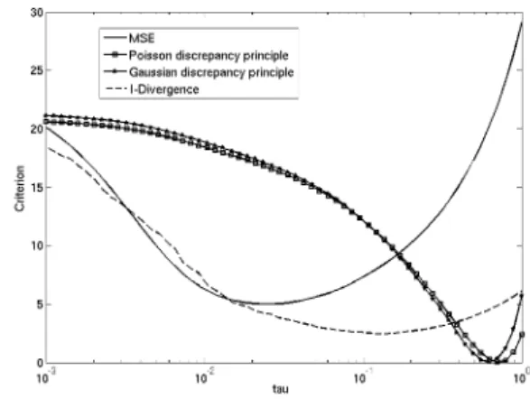
where x is the given synthetic original image. Figure 2 and table 1 show the estimation of the regularizing parameter for the image (a). This image is a high intensity image with a constant background b = 1. On this image, the estimators (11) and (17) give values which are actually very close to the value given by the minimization of the I-Divergence (see table 1). They are a little higher than the value given by the minimization the MSE, this is however still acceptable as the obtained restored images only slightly differ. Figure 3 and table 1 show the estimation of the regularizing parameter for the image (b). This image is also a high inten-sities image but with a null background which is a frequent property of biomedical and astrophysics images for example. In this configuration, the constraint x≥ 0 in the restoration algorithm (5) is changed to x ≥ ǫ, where ǫ is a small con-stant, to prevent numerical issues in the computation of the estimators (11) and (17). We will show in the next section
(a) (b)
(c) (d)
Figure 1: Synthetic 2D images. The first row is the observed images (Poisson noise and blur) while the second row is the original images.
Figure 2: Estimation of τ on the image (a) of the figure 1
how to deal with these images with still keeping the con-straint x≥ 0 in the restoration algorithm. On this image, estimators (17) and (11) fail to give acceptable estimation of the regularizing parameter (see table 1). The error of esti-mation is very important and this could be explained by the fact that this image actually contains many zero-valued pix-els (about 65% of the whole number of pixpix-els) and that the estimators (17) and (11) do not take into account this kind of property. We propose in the next section a modification of these estimators to address this issue.
3.
PROPOSED METHOD
We show in the next lines that we can improve the accuracy of these estimators by taking into account the properties of the application. For example, images in biology often contain many pixels where the number of collected photons is zero. For this reason, we propose to split the domain Ω in several sub-domains and to compute each estimator on
❳ ❳ ❳ ❳ ❳ ❳ ❳ ❳❳ Criterion Image (a) (b) Gaussian discrepancy principle (11) 0.153 0.626 Poisson discrepancy principle (17) 0.122 0.703 MSE (20) 0.076 0.026 I-Divergence (19) 0.121 0.108 Table 1: Values of the estimated regularizing pa-rameter on images (a) and (b) of the figure 1 for the estimators (11), (17) and comparison to measures (20) and (19).
Figure 3: Estimation of τ on the image (b) of the figure 1
these sub-domains.
3.1
Notations
We recall that our model writes:
y =P(λ), (21) with λ = Hx + b. Let us define the index sets Θ1 ={i ∈
Ω|yi > 0} and Θ0 ={i ∈ Ω|yi = 0}. Same definitions are
applied to λ and give the index sets Λ1 ={i ∈ Ω|λi > 0},
Λ0={i ∈ Ω|λi= 0}. We have Ω = Θ1∪ Θ0= Λ1∪ Λ0.
Let us also define any combination of these index sets :
• S0= Θ0∩ Λ0,
• S1= Θ0∩ Λ1,
• S2= Θ1∩ Λ0,
• S3= Θ1∩ Λ1.
Firstly remark that S2is empty by definition (21). Secondly,
note that these sets do not overlap and that we also have Ω = S0∪ S1∪ S3.
3.2
Gaussian approximation
We first consider the Gaussian approximation (6). We recall that the authors of [1] have proposed to write:
with:
e = (ei)i∈Ωand ei∼ N (0,√yi) ∀i ∈ Ω. (23)
However, we may use the decomposition of Ω over the index sets Si, i∈ {0, 1, 3} to refine the previous assumption:
• ei= 0 ∀i ∈ S0 by definition (1).
• On the domain S1, eiis fully determinist and given by
ei=−(Hx + b)iwhich unfortunately needs to be
esti-mated from real data as the true image x is unknown. • On S3, the previous assumption is valid and writes
ei∼ N (0,√yi).
Observe that S1 actually represents elements with very low
intensities which give zero-valued observed pixels and mostly appears on the object borders in the image, due to the con-volution effect which spreads these borders giving very small intensities. Values of eion this domain should therefore be
very small. Not taking into account this domain should not increase the estimation error too much for images with suf-ficient “large” objects as the number of disregarded compo-nents card(S1) is very small with respect to card(S3). Note
that this assumption is however false for images containing only thin structures like points or filaments. For all other images, we propose consequently to write that:
e = (ei)i∈Ωand ( ei∼ N (0,√yi) ∀i ∈ S3 ei= 0 otherwise . (24) In this case r(x)∼ N (0, Σ): Σ = (Σi)i∈Ωwith Σi= (√ yi if i∈ S3 0 otherwise , (25) such that we have:
r(x) = (
(Hx− (y − b)) /√y if i∈ S3
0 otherwise . (26) Consequently, we rewrite (8) as:
kr(x)k22∼ χ2(card(S3))) = χ2(card(Θ1)) = χ2(m), (27)
where m = card(Θ1) actually represents the number of
strictly positive pixels in the observation y. Following this last equation, we propose to select the regularizing parame-ter τ such that it verifies:
τopt= arg min n ˜Ψy(x∗τ)− 1
o2 subject to τ ∈ R+ , (28) where: ˜ Ψy(x) = 1 m ‚ ‚ ‚(H x − (y − b)) / √ Hx + b‚‚ ‚ 2 2. (29)
Note that due to the splitting of the domain, we can main-tain the constraint x≥ 0 in the restoration algorithm as we compute the estimator only for strictly positive pixels val-ues. We see in the next section how to apply the same idea to the Poisson discrepancy principle.
3.3
Poisson discrepancy principle
The authors of [2] have computed their estimator on the whole index set Ω and have found that :
E(JL(x, y)) = 1 2 X i∈Ω E(F (xi, yi))≃ 1 2card(Ω) = n 2 (30) As previously, we may use the decomposition of Ω over the index sets Si, i∈ {0, 1, 3} to refine the computation of the
expected value. Indeed : E(JL(x, y)) = 1 2 X i∈Ω E(F (xi, yi)) = 1 2 “ X i∈S0 E(F (xi, yi))+ X i∈S1 E(F (xi, yi)) + X i∈S3 E(F (xi, yi)) ” = E0+ E1+ E3. (31) We now detail the computation of each term Ei, i∈ {0, 1, 3}:
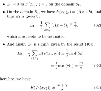
• E0= 0 as F (xi, yi) = 0 on the domain S0.
• On the domain S1, we have F (xi, yi) = (Hx + b)iand
thus E1 is given by:
E1= 1 2 X i∈S1 (Hx + b)i, γ 2, (32) which also needs to be estimated.
• And finally E3 is simply given by the result (16):
E3= 1 2 X i∈S3 E(F (xi, yi))≃ 1 2card(S3) =1 2card(Θ1) = m 2 (33) Therefore, we have: E(JL(x, y))≃ m + γ 2 (34)
Following the same approximation than the one in the sec-tion 3.2, we propose to disregard the effect of γ in front of m and propose:
E(JL(x, y))≃
m
2 (35)
Finally, the regularizing parameter should be chosen as: τopt= arg min n ˜Υy(x∗τ)− 1
o2 subject to τ∈ R+ , (36) where: ˜ Υy(x) = 2 m X i∈Ω
(Hx + b)i−yi+yilog(yi)−yilog [(Hx + b)i] .
(37)
3.4
Results
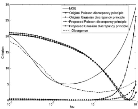
Figure 4 and table 2 show the estimation of the modified estimators for the image (b) of the figure 1. Values are compared to original estimators [1] and [2]. We see that the estimation error has been strongly reduced using the proposed estimators. On this image, estimated values are now in between the values given by the MSE and the I-Divergence.
Figure 4: Estimation of τ on the image (b) of the figure 1
Gaussian discrepancy principle (11) 0.626 Poisson discrepancy principle (17) 0.703 Proposed Gaussian discrepancy principle (28) 0.042 Proposed Poisson discrepancy principle (36) 0.037
MSE (20) 0.026
I-Divergence (19) 0.108 Table 2: Values of the estimated regularizing param-eter on image (b) of the figure 1 for the estimators (11), (17), the proposed modifications (28), (36) and comparison to measures (20) and (19).
4.
CONCLUSIONS
We have proposed two estimators to select the regularizing parameter for the deconvolution of images corrupted by blur and Poisson noise. Values given by these estimators have been compared to classical image fidelity measures and have shown promising results. Future works will be focused on the accuracy of the estimators and on the validity of the ap-proximations made for images containing only thin objects like points or filaments.
5.
ACKNOWLEDGMENTS
This research work has been funded by the ANR DetectFine.
6.
REFERENCES
[1] J. M. Bardsley and J. John Goldes. Regularization parameter selection methods for ill-posed poisson maximum likelihood estimation. Inverse Problems, 25(9), 2009.
[2] M. Bertero, P. Boccacci, G. Talenti, R. Zanella, and L. Zanni. A discrepancy principle for poisson data. Inverse Problems, 26(10), 2010.
[3] I. Csisz´ar. Why least squares and maximum entropy? The Annals of Statistics, 19:2032–2066, 1991. [4] A. P. Dempster, N. M. Laird, and D. B. Rubin.
Maximum Likelihood from Incomplete Data via the EM Algorithm. Journal of the Royal Statistical Society. Series B (Methodological), 39(1):1–38, 1977. [5] N. Dey, L. Blanc-F´eraud, C. Zimmer, Z. Kam,
P. Roux, J. C. Olivo-Marin, and J. Zerubia.
Richardson-lucy algorithm with total variation regularization for 3d confocal microscope deconvolution. Microscopy Research Technique, 69:260–266, 2006.
[6] F.-X. Dup´e, J. Fadili, and J.-L. Starck. A proximal iteration for deconvolving poisson noisy images using sparse representations. IEEE Transactions on Image Processing, 18(2):310–321, Feb. 2009.
[7] M. A. T. Figueiredo and J. M. Bioucas-Dias. Restoration of poissonian images using alternating direction optimization. IEEE Transactions on Image Processing, 19(12):3133–3145, Jan. 2010.
[8] K. Lange and R. Carson. EM reconstruction
algorithms for emission and transmission tomography. Journal of Computer Assisted Tomography,
8(2):306–316, Apr. 1984.
[9] L. B. Lucy. An iterative technique for rectification of observed distributions. The Astronomical Journal, 79(6):745–765, 1974.
[10] N. Pustelnik, C. Chaux, and J.-C. Pesquet. Hybrid regularization for data restoration in the presence of Poisson noise. In 17th European Signal Processing Conference (EUSIPCO’09), Aug. 2009.