HAL Id: hal-01966006
https://hal.archives-ouvertes.fr/hal-01966006
Submitted on 27 Dec 2018
HAL is a multi-disciplinary open access
archive for the deposit and dissemination of
sci-entific research documents, whether they are
pub-lished or not. The documents may come from
teaching and research institutions in France or
abroad, or from public or private research centers.
L’archive ouverte pluridisciplinaire HAL, est
destinée au dépôt et à la diffusion de documents
scientifiques de niveau recherche, publiés ou non,
émanant des établissements d’enseignement et de
recherche français ou étrangers, des laboratoires
publics ou privés.
Constrained Kaczmarz’s Cyclic Projections for
Unmixing Hyperspectral Data
Paul Honeine, Henri Lantéri, Cédric Richard
To cite this version:
Paul Honeine, Henri Lantéri, Cédric Richard. Constrained Kaczmarz’s Cyclic Projections for
Unmix-ing Hyperspectral Data. Proc. 21th European Conference on Signal ProcessUnmix-ing (EUSIPCO), 2013,
Marrakech, Morocco. pp.1-5. �hal-01966006�
CONSTRAINED KACZMARZ’S CYCLIC PROJECTIONS FOR UNMIXING
HYPERSPECTRAL DATA
Paul Honeine
Institut Charles Delaunay (CNRS)
Université de technologie de Troyes
Troyes, France
[email protected]
Henri Lantéri, Cédric Richard
Laboratoire Lagrange (CNRS)
Université de Nice Sophia-Antipolis
Nice, France
{henri.lanteri, cedric.richard}@unice.fr
ABSTRACT
The estimation of fractional abundances under physical con-straints is a fundamental problem in hyperspectral data pro-cessing. In this paper, we propose to adapt Kaczmarz’s cyclic projections to solve this problem. The main contribution of this work is two-fold: On the one hand, we show that the non-negativity and the sum-to-one constraints can be easily imposed in Kaczmarz’s cyclic projections, and on the sec-ond hand, we illustrate that these constraints are advantageous in the convergence behavior of the algorithm. To this end, we derive theoretical results on the convergence performance, both in the noiseless case and in the case of noisy data. Exper-imental results show the relevance of the proposed method.
Index Terms— Constrained optimization, Kaczmarz’s cyclic projections, hyperspectral data, unmixing problem
1. INTRODUCTION
Due to low spatial resolution of hyperspectral cameras (i.e., imaging spectrometers), acquired spectra are mixtures of spectra of some pure materials. These pure components are also called endmembers. The unmixing problem consists of breaking down a spectrum into the pure spectra of endmem-bers and their fractional abundances. A wide range of geo-metrical and statistical methods has been devised for the un-mixing problem. See [2] for an extensive overview. Hyper-spectral data processing often suffers from a number of limi-tations, which includes computation complexity and the ease of implementation, making iterative and parallel algorithms suitable for implementation [7, 1].
Assuming that the endmembers were extracted using any off-the-shelf technique, the problem of estimating the frac-tional abundances provides new opportunities and challenges to both linear [9] as well as non-linear unmixing problems [4]. In order to have a coherent physical interpretation, two hard constraints need to be satisfied in the estimation problem: the
This work was supported by the French ANR, grant HYPANEMA: ANR-12-BS03-0003.
sum-to-one of all the fractional abundances and there non-negativities. In this work, we study the problem of estimat-ing constrained fractional abundances, by suitably adaptestimat-ing a cyclic orthogonal projection scheme.
Methods of orthogonal projections onto spaces, and more recently onto convex sets, have been successfully applied for solving many optimization problems, in the field of sig-nal processing in particular. These methods include the cel-ebrated Cimmino’s parallel projections [5] and Kaczmarz’s cyclic projections [10]. More recently, projections onto spaces have been generalized to projections onto convex sets. These methods provide a unified framework for tackling many signal processing problems, including adaptive filtering and machine learning [14, 13]. To the best of our knowl-edge, these methods have not yet been exploited in hyper-spectral image processing. Very recently, we have success-fully adapted Cimmino’s parallel projections [5] for the hy-perspectral unmixing problem [8].
Coupled with these advances, this paper shows that the spectral unmixing problem can take advantage of these devel-opments. To this end, we propose to adapt Kaczmarz’s cyclic projection for estimating the fractional abundances. Appro-priate strategies for enforcing the non-negativity and sum-to-one constraints are advanced as a natural extension of the con-ventional unconstrained Kaczmarz’s method: the sum-to-one constraint is enforced by a projection scheme, while the non-negativity is satisfied by relaxing the projections.
2. THE LINEAR UNMIXING MODEL
Given a spectrum withL wavelength x = [x1 x2 · · · xL]!
(e.g. a pixel in a hyperspectral image), the linear mixing model takes the form
M α= x + ", (1) where M is theL-by-K matrix of the K spectral signatures of a pure material, i.e., endmember, and " is the vector of fitness error, and α is the vector ofK abundances to be de-termined. In this work, we assume that the endmembers have
been properly identified, using a supervised or an unsuper-vised endmember extraction technique. The paper [2] pro-vides an extensive overview of existing techniques and state-of-the-art methods.
To adopt a physical interpretation of the unmixing prob-lem, the linear combination in model (1) needs to be convex. In other words, the following constraints are required:
• The sum-to-one of the contributions, 1!α = 1, where
1denotes the unit column-vector ofK entries; • and the non-negativity of the contributions, α ≥ 0,
where the inequality is taken component-wise. An iterative scheme is required to solve the constrained opti-mization problem: arg minα"Mα − x"
2, under the above
constraints. See for instance [6].
3. CONSTRAINED KACZMARZ’S CYCLIC PROJECTIONS
To revisit the unconstrained Kaczmarz’s method, we consider the noiseless model, defined by
M α= x. (2)
In other words, Kaczmarz’s method assumes that x belongs to the range of the matrix M . The impact of the presence of noise, as given in model (1), is studied in next Section.
3.1. Unconstrained Kaczmarz’s cyclic projections The linear system (2) ofL equations and K unknowns gives rise to a set ofL affine hyperplanes,
H!= ! α""" m! !α= x! # . (3)
In this expression, m!! denotes the!-th row of M , namely the
spectral signatures of the endmembers at the!-th wavelength band. The solution of the linear system (2) is the intersection of theL affine hyperplanes, i.e., H1∩H2∩. . .∩HL, where the
intersection is a unique point in the noiseless case. It is worth noting that M is full column rank by construction, since non of the endmembers can be written as a linear combination of other endmembers.
The conventional Kaczmarz’s method sweeps through the affine hyperplanes, by projecting orthogonally onto each and taking this as the next iterate. In a mathematical form, at the t-th iteration, t-the projection of αt−1onto the affine hyperplane
H!reads αt−1⊥!= αt−1+x!− m ! ! αt−1 "m!"2 m!, (4)
with α0 some initial guess. This process is iterated until a
given convergence criterion is satisfied. In this expression,!
1 H m! H! αt−1 αt−1⊥! αt θ! αopt
Fig. 1. Illustration in two-dimensions of the constrained Kacz-marz’s cyclic projections. The affine hyperplane of the sum-to-one constraint is H (black line), i.e., the hyperplane defined by the nor-mal vector 1.
is selected at each iterationt, i.e., a slight abuse of notation is made in using! rather than !(t).
Several strategies [11, 12, 3] have been proposed to choose the sequence of selected affine hyperplanes, i.e., the choice at iterationt of the !-th row in the matrix M . The classical cyclic selection, i.e.,! = t mod L, is the simplest one; however it could lead to low convergence. Other strate-gies have been proposed to overcome this drawback, the most known are the maximum error selection and the randomiza-tion. The maximum error selection requires the evaluation of the numerator in (4) for all! at each iteration t, which leads to a high computational burden. In randomization! is chosen randomly with probability proportional to the denominator in (4), i.e., "m!"2. This strategy has shown very interesting
properties [12], but is also criticized in [3].
This paper shows that, in the case of a constrained solu-tion as in the unmixing problem, Kaczmarz’s method does not suffer from the problem of appropriate selection of the affine hyperplanes. Moreover, we provide theoretical results on the convergence, for the noiseless and the noisy cases.
3.2. Sum-to-one constraint
To impose the sum-to-one constraint, we consider a two-step strategy at each iterationt: a projection of αt−1 onto the
affine hyperspaceH!, yielding αt−1⊥!, followed by a
nor-malization to satisfy the constraint, yielding αt. The
pro-posed strategy is illustrated in Figure 1.
LetH be the affine hyperplane defined by the sum-to-one, namelyH = $α| 1!α= 1%. By analogy with the expres-sion of the projection (4), the normalization of any αt−1⊥!is
given by
αt= αt−1⊥!+ 1
K
&
1 − 1!αt−1⊥!'1, (5) where m!is now substituted with 1, the unit column-vector
ofK ones. By combining this projection (5) with the projec-tion ontoH!, as given in (4), at iterationt, we get:
αt = αt−1⊥!+ 1 K & 1 − 1!αt−1+⊥!'1 = αt−1+x!− m ! ! αt−1 "m!"2 m! +K1 ( 1 − 1!αt−1−x!− m ! ! αt−1 "m!"2 1!m! ) 1.
Since we have the identity 1!αt−1 = 1 from the previous iteration, we obtain the following update rule:
αt= αt−1+x!− m ! ! αt−1 "m!"2 & I− 1 K11 !'m !. (6)
Here, I denotes the matrix identity of sizeK-by-K, and the matrix I− 1
K11
! is often called centering matrix in the
ma-chine learning literature.
It is worth noting that there is another way to satisfy the sum-to-one constraint, by normalizing using the form:
αt= αt−1⊥! 1!αt−1⊥!.
This normalization can also be viewed as a non-orthogonal projection, and therefore looses the property of nonexpansive transformation. Technically, this means that the distance be-tween two projections may exceed the distance bebe-tween the two original elements, and therefore compromising the speed of convergence. For these reasons, this normalization is not considered in this paper, as we adopt the (orthogonal) projec-tion given in (5).
3.3. Imposing also the non-negativity constraint
To enforce the non-negativity constraint, namely αt ≥ 0 at
each iteration, we propose to relax the projection in (6), by considering the following update rule:
αt= αt−1+ ηt x!− m ! ! αt−1 "m!"2 &I − 1 K11 !'m !. (7)
The relaxation parameterηt ∈ [0 ; 1] is chosen in order to
impose the non-negativity of entries in αt.
To this end, let
ηt= min i=1,...,Kη
(i) t ,
whereη(i)t is a valid stepsize in thei-th direction. The value
of the latter depends on one of the two cases: • If x!−m!! αt−1 $m!$2 *&I − 1 K11 !'m !+i > 0, there is no
constraint on the stepsize, and therefore could be set toη(i)t = 1;
• Otherwise, the stepsize should be reduced such that ηt(i)≤ [αt−1]i !" I−K 111 !#m! $ i .
In order to account for noise, we consider always a relaxation of the projection. The stepsize is set to a smaller value than one (e.g.,0.1 or below depending on the above relations), as recommended in adaptive filtering literature. Essentially, the update rule (7) is a normalized least mean squares (NLMS) algorithm applied on centered data.
Other strategies to enforce the non-negativity constraint can also be applied, such as a post-processing by replacing every negative entry in αtwith zero. However, this strategy of
projection onto the positive half-space may destroy the sum-to-one constraint, and therefore it is not recommended.
4. THEORETICAL RESULTS
In this section, we provide theoretical results, namely on the convergence rate in both the noiseless (2) and the noisy cases (1). To this end, we consider the influence of both sum-to-one and non-negativity constraints by using the update rule (7).
First of all, the impact of the non-negativity constraint is clear. All the results are enforced to be on the non-negative orthant in theK-dimensional space. Furthermore, the studied hyperspectral unmixing problem has the following interest-ing property: Since m! is a vector of values from spectral
signatures at the !-th wavelength band, we have m! ≥ 0,
and therefore all affine hyperplanes defined by (3) have non-negative normal vectors. Moreover, the sum-to-one affine hy-perplaneH is the bisector of the orthant, and therefore the angle between it and anyH!cannot exceed π/4. Let θ!be
the angle between the two affine hyperplanesH!andH, then
cos(θ!) > 1/
√
2, for all ! = 1, 2, . . . , L.
Let αoptbe the (unknown) optimal solution of the
noise-less problem (2).
4.1. The noiseless case
The following theorem provides the rate of convergence for the proposed constrained Kaczmarz’ method, in the case of the noiseless model (2). To this end, we consider the influence of the sum-to-one constraint on the convergence.
Theorem 1 (Convergence in the noiseless case).
Starting from an initial guess α0, the algorithm converges to
the optimal solution αoptat the rate
"αt− αopt" = "α0− αopt"
,
!(t#)
t#≤t
cos2(θ!),
whereθ!is the angle betweenH!andH, and the product is
Proof. As in the conventional Kaczmarz’s method, it is as-sumed that the solution of the linear system exists, is unique, and belongs to the setH!. On the one hand, we have from
projection (i.e., according to the Pythagorean theorem) cos(θ!) ="α
t−1⊥!− αopt"
"αt−1− αopt"
,
wherecos(θ!) is positive as discussed above. On the other
hand, we also have
cos(θ!) = "α
t− αopt"
"αt−1⊥!− αopt".
By combining both expressions, we get
"αt− αopt" = "αt−1⊥!− αopt" cos(θ!)
= "αt−1− αopt" cos2(θ!) .. . = "α0− αopt" , !(t#) t#≤t cos2(θ!).
This concludes the proof.
This theorem demonstrates the rate of convergence of the proposed algorithm. It is worth noting thatcos(θ!) can be
eas-ily evaluated, sincecos(θ!) = 1
!m!
$1$$m!$, where the numerator
is the sum of the entries of m!, and the denominator involves
the sum of their squares.
Moreover, each iteration in the proposed algorithm is essentially a double projection. This alternating projection can be applied infinitely on a fixed!, i.e., affine hyperplane H!, without the need to sweep through all the affine
hyper-planes. In this case, the Theorem 1 becomes for a fixed!: "αt− αopt" = "α0 − αopt" (cos(θ!))2t. In practice, due
to the presence of noise, it is not enough to use a single!, but rather to sweep over all the hyperplanes. The next Sec-tion provides a study of the impact of noise on the proposed algorithm.
4.2. The noisy case
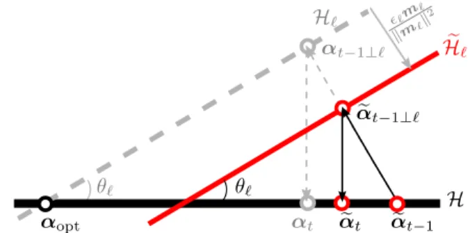
Very few works consider the influence of noise in the con-ventional (unconstrained) Kaczmarz’s cyclic projections. The presence of noise is seldom considered; see [11] for the ran-domized Kaczmarz’s method. In this section, we provide a theoretical analysis of the presence of an error in the pro-posed constrained optimization problem. We assume that the endmember spectra have been well estimated, and the noise is on the investigated spectrum as given in (1), namely M α= x + ", where " = [%1%2 . . . %L]!is the error vector. The solution of this noisy problem belongs to the intersec-tion of theL affine hyperplanes -H1∩ -H2∩ . . . ∩ -HL, defined
by -H!= ! α""" m! !α= x!+ %! # . H H! -H! -αt−1 -αt−1⊥! αt−1⊥! -αt αt "!m ! $m !$ 2 θ! θ! αopt
Fig. 2. Illustration in two-dimensions of the presence of noise. In this case,H! is not available (neither all gray
el-ements), but the affine hyperplane -H!associated to the noisy
data. Therefore, at instantt−1, the approximation -αt−1leads toα-t, rather than αt.
It is easy to see that these affine hyperplanes can also be de-fined from the hyperplanes associated for the noiseless case, with (See for instance [11, Lemma 2.2]):
-H!= ! α+ "! $m!$2 m! " " " α ∈ H! # . (8)
Letα-t−1 be the estimate obtained at iterationt in presence of noise, andα-t−1⊥!its projection onto -H!. The following theorem is a generalization of Theorem 1 to the case of noisy data. See Figure 2 for an illustration.
Theorem 2 (Convergence in the noisy case). Starting from an initial guessα-0, the algorithm converges at the rate
"-αt− αopt"2 = "-α0− αopt"2, !(t#) t#≤t cos4(θ!) +. !(t#) t#≤t %2 ! "m!"2 cos2(θ!) , !(t##) t##<t# cos4(θ!##),
whereθ!is the angle betweenH and H!(as well as -H!).
Proof. First, we have from projection the following relation: cos(θ!) = "-αt− αopt"/"-αt−1⊥!− αopt". By applying the
Pythagorean theorem, the above denominator can be decom-posed into
"-αt−1⊥!− αopt"2= "αt−1⊥!− αopt"2+ " "!
$m!$2
m!"2,
where the orthogonality and the definition (8) are used. The second term in the right-hand-side is simply%2
!/"m!"2. The
first term in the right-hand-side is (see the proof of Theo-rem 1): "αt−1⊥!− αopt" = "-αt−1 − αopt" cos(θ!). By
combining these expressions, we get
"-αt− αopt"2="-αt−1− αopt"2cos4(θ!) + %
2 ! "m!"2 cos2(θ!) .. . ="-α0− αopt"2, !(t#) t#≤t cos4(θ!) +. !(t#) t#≤t %2 ! "m!"2 cos2(θ!) , !(t##) t##<t# cos4(θ!#).
This concludes the proof.
This theorem demonstrates the impact of the selection, i.e.,!(t) at each iteration t, on the approximation error. In fact, thanks to the geometric progression of the cosines, the hyperplanes considered in the first iterations have their errors highly reduced, as opposed to the last projections with less “cosine” weights. In other words, it is clear that the band-widths in the hyperspectral data with the largest errors, i.e., large values of%2
!/"m!"2, should be used in the first
itera-tions. Therefore, this theorem provides a new selection cri-terion for the cyclic projections, optimal for the studied con-strained optimization problem.
5. EXPERIMENTATIONS
The proposed learning algorithm was used for hyperspectral data unmixing, generated by a linear combination of three pure materials with abundanceα = [0.4 0.65 − 0.05]!,
where we injected a sign error on the third abundance. These materials are grass, cedar and asphalt, with spectral signa-tures extracted from the USGC library. These spectra con-sist of 2151 bands covering wavelengths ranging from 0.35 to 2.5µm. The data were corrupted by an additive Gaussian noise. Figure 3 illustrates the convergence of the proposed al-gorithm, for a SNR of≈ 25 dB and ≈ 18 dB, with the largest value of the stepsize fixed to0.1 and a single sweep over all the bandwidths. For a comparative results, we also show in the same figure the estimates using non-negative least-squares and the fully-constrained least-squares techniques [6].
6. CONCLUSION AND PERSPECTIVES In this paper, we presented the development of a new class of unmixing methods, by providing constrained counterpart of projection-based algorithms [14, 13]. New theoretical re-sults were derived for the studied constrained optimization problem, including the impact of noise on the analyzed spec-trum. Experimentations collaborate these results. As for fu-ture work, we seek to study the impact of noise on the end-members. We are also conducting a statistical analysis on the impact of noise, as well as connections with adaptive filtering.
SNR ≈25dB SNR ≈18dB 0 200 400 600 800 100012001400160018002000 −0.1 0 0.1 0.2 0.3 0.4 0.5 0.6 0.7 iterations over ! α t 0 200 400 600 800 100012001400160018002000 −0.1 0 0.1 0.2 0.3 0.4 0.5 0.6 0.7 iterations over ! α t
Fig. 3. Convergence of the constrained Kaczmarz’s optimization method, for a mixture of two spectra with additive noise. The dotted lines correspond to the real abundances α= [0.4 0.65 −0.05]
!.
The estimates using non-negative least-squares (given by “+”) and the fully-constrained least-squares (given by “!”) are also given.
7. REFERENCES
[1] J. Bioucas-Dias and M. Figueiredo. Alternating direction algorithms for con-strained sparse regression: Application to hyperspectral unmixing. In Proc. 2nd IEEE Workshop on Hyperspectral Image and Signal Processing : Evolution in Remote Sensing (WHISPERS), Reykjavik, Iceland, 2010.
[2] J. M. Bioucas-Dias, A. Plaza, N. Dobigeon, M. Parente, Q. Du, P. Gader, and J. Chanussot. Hyperspectral unmixing overview: Geometrical, statistical, and sparse regression-based approaches. IEEE J. Sel. Topics Appl. Earth Observations and Remote Sens., 5(2):354–379, April 2012.
[3] Y. Censor, G. T. Herman, and M. Jiang. A note on the behavior of the random-ized Kaczmarz algorithm of Strohmer and Vershynin. J. Fourier Anal. Appl., 15(4):431–436, 2009.
[4] J. Chen, C. Richard, and P. Honeine. Nonlinear unmixing of hyperspectral data based on a linear-mixture/nonlinear-fluctuation model. IEEE Transactions on Sig-nal Processing, 61(2):480–492, January 15 2013.
[5] G. Cimmino. Calcolo approssimato per le soluzioni dei sistemi di equazioni lin-eari. La Ricerca Scientifica, II, 9:326–333, 1938.
[6] D. Heinz and C. Chang. Fully constrained least squares linear spectral mixture analysis method for material quantification in hyperspectral imagery. IEEE Trans. Geoscience and Remote Sensing, 39(3):529–545, March 2001.
[7] R. Heylen, D. Burazerovic, and P. Scheunders. Fully constrained least-squares spectral unmixing by simplex projection. IEEE Transactions on Geoscience and Remote Sensing, 49(11):4112–4122, 2011.
[8] P. Honeine and H. Lantéri. Constrained reflect-then-combine methods for unmix-ing hyperspectral data. In Proc. IEEE Workshop on Hyperspectral Image and Sig-nal Processing : Evolution in Remote Sensing (WHISPERS), Gainesville, Florida, USA, 25 - 28 June 2013.
[9] P. Honeine and C. Richard. Geometric unmixing of large hyperspectral images: a barycentric coordinate approach. IEEE Transactions on Geoscience and Remote Sensing, 50(6), June 2012.
[10] S. Kaczmarz. Angenäherte Auflösung von Systemen linearer Gleichungen. Bul-letin International de l’Académie Polonaise des Sciences et des Lettres, 35:355– 357, 1937.
[11] D. Needell. Randomized Kaczmarz solver for noisy linear systems. BIT Numeri-cal Mathematics, 50(2):395–403, June 2010.
[12] T. Strohmer and R. Vershynin. A randomized Kaczmarz algorithm with exponen-tial convergence. J. Fourier Anal. Appl., 15(2):262–278, 2009.
[13] S. Theodoridis, K. Slavakis, and I. Yamada. Adaptive learning in a world of pro-jections. IEEE Signal Processing Magazine, 28(1):97–123, 2011.
[14] M. Yukawa. Adaptive filtering based on projection method. Lecture Notes, De-cember 6–8, 2010.