HAL Id: cea-01888831
https://hal-cea.archives-ouvertes.fr/cea-01888831
Submitted on 5 Oct 2018
HAL is a multi-disciplinary open access
archive for the deposit and dissemination of
sci-entific research documents, whether they are
pub-lished or not. The documents may come from
teaching and research institutions in France or
abroad, or from public or private research centers.
L’archive ouverte pluridisciplinaire HAL, est
destinée au dépôt et à la diffusion de documents
scientifiques de niveau recherche, publiés ou non,
émanant des établissements d’enseignement et de
recherche français ou étrangers, des laboratoires
publics ou privés.
Anomaly Detection in Vehicle-to-Infrastructure
Communications
Michele Russo, Maxime Labonne, Alexis Olivereau, Mohammad Rmayti
To cite this version:
Michele Russo, Maxime Labonne, Alexis Olivereau, Mohammad Rmayti. Anomaly Detection in
Vehicle-to-Infrastructure Communications. 2018 IEEE 87th Vehicular Technology Conference (VTC
Spring), Jun 2018, Porto, Portugal. �10.1109/VTCSpring.2018.8417863�. �cea-01888831�
Anomaly Detection in
Vehicle-to-Infrastructure Communications
Michele Russo, Maxime Labonne, Alexis Olivereau, Mohammad Rmayti
LIST, Communicating Systems Lab 91191 Gif-sur-Yvette CEDEX, France
{michele.russo, maxime.labonne, alexis.olivereau, mohammad.rmayti}@cea.fr
Abstract— This paper presents a neural network-based anomaly detection system for vehicular communications. The proposed system is able to detect in-vehicle data tampering in order to avoid the transmission of bogus or harmful information. We investigate the use of Long Short-term Memory (LSTM) and Multilayer Perceptron (MLP) neural networks to build two prediction models. For each model, an efficient architecture is designed based on appropriate hardware requirements. Then, a comparative performance analysis is provided to recommend the most efficient neural network model. Finally, a set of metrics are selected to show the accuracy of the proposed detection system under several types of security attacks.
Keywords—Anomaly detection; LSTM; MLP; V2I; forecasting; benchmarking.
I. INTRODUCTION
Over the last decade, most of intra-vehicular communications in automotive systems were based on so-called Electronics Control Units (ECU). More recently, connected automotive networking services were introduced, involving Vehicle-to-Vehicle (V2V) and Vehicle-to-Infrastructure (V2I) communications. This growth of networking capability [1], [2], [3] was accompanied with some security flaws that expose the vehicles to cyber-attacks [4], [5], [6], [7]. For instance, packet injection and data manipulation attacks can threat some critical components that are responsible of driver’s safety services. On other hand, several anomalies can arise in case of harmful incidents such as malfunctions, human errors or signals interruptions. This highlights the relevance of anomaly detection in the automotive environment.
By definition, an anomaly-based Intrusion Detection System (IDS) collects and analyzes information about computer or network system in order to detect anomalies that can disturb its normal activity. In automotive systems, data that are collected from various in-vehicle sensors and ECUs are transmitted to the infrastructure (e.g., the cloud) in the form of sequences of observations. Then, this information being processed and used by critical applications should be protected against forging and tampering attacks.
The objective of this paper is therefore to design an anomaly-based IDS for Vehicle-to-Cloud (V2C) communications. In order to detect anomalies in the V2I data sequence, a neural network-based anomaly detector is designed to be implemented
in the vehicle’s gateway. It raises an alert whenever the data received from the sensors are classified as anomalous.
The rest of this paper is organized as follows. Section II discusses some related works in particular those focusing on sequence anomaly detection. Section III introduces the two studied neural network models and the experimental setup used to assess them. Section IV details the experiments that were carried out to evaluate their performance in terms of resource efficiency and attack detection quality. Section V concludes the paper.
II. STATE OF THE ART
Many approaches have been applied to anomaly detection in sequences [8]. A common approach is to identify and compare patterns in n-grams, where an n-gram is a length-n subsequence. Many algorithms were used to measure the distance between candidate n-grams and historical n-grams or other parts of the same sequence (e.g., [9]). These methods are difficult to apply on the values collected from vehicle’s sensors, because they assume a finite symbol dictionary, or rely on some quantization methods to convert continuous values to a finite set of symbols. Since sensors’ data are continuous, it is not possible to rely on foreign symbols (i.e., values) to detect anomalies. Similarly, Hidden Markov Models could theoretically be used, but would need to be adapted to work on a compressed representation of data. Their performance would then be dependent on the quality of the chosen compression algorithm.
Several machine learning and statistical approaches for anomaly detection on continuous sequences (or time series), have been proposed in the literature: Recurrent Neural Network (RNN)-based [10], LSTM-based forecasting and encoder-decoder [11], [12], [13], clustering based [14], (Demixed) Principal Component Analysis, Linear Discriminant Analysis [15], one-class Support Vector Machine (SVM) and segmentation [16], change point detection [17] and MLP [29], [30]. Each of these systems tries to predict the next symbol in the sequence. Anomalies are detected when the distance between predicted and actual data exceeds a defined threshold.
The usage of LSTM for forecasting has especially been shown to be very effective in standard time series test sets [18], electrocardiography [19], aircraft telemetry [20] and automotive [21], [22].
III. USE CASE,ASSUMPTIONS AND EXPERIMENTAL SETUP
A. Design Decisions for Anomaly Detection
The anomaly detection method that we use in this work is based on forecasting. This class of anomaly detection algorithms uses past data to predict current data, and measures the difference between observed data and their prediction. By this definition, forecasting relies on supervised machine learning, since it trains a regression model of data values versus time. Predictions performed by a forecasting model will correspond to the expected value that a time series will have in the next time step. Hence, forecasting can particularly fit the data format in the considered use case, namely, an ordered sequence of data packets. In addition, using such predictor does not require any knowledge about abnormalities to work, which will be proved throughout this study, where the available datasets contain only real non-anomalous data.
We compared two neural network models for forecasting. The first one is based on LSTM neural networks, which shown a high efficiency for time-series forecasting in a variety of domains especially in automotive scenarios. The second type that we considered in this study is MLP-based neural networks is based on the MLP architecture, which was widely used for time series forecasting in the early days of machine learning [23]. In fact, the MLP is a lightweight model in terms of hardware infrastructure requirements, training phase duration and resource consumption, which is adapted for automotive environment. In addition, recent studies showed that a time window based MLP can outperform the LSTM on certain time-series prediction benchmarks bas on few recent inputs [24].
B. Training and Testing
The available data was captured within a 2010 Toyota Prius 3 vehicle, equipped with components for automated/cooperative driving and standard vehicle sensors. The final dataset contains almost 650 thousands packets collected during approximately 7 hours of driving. Based on these datasets, 20% of packets (i.e., about 1.5 hours of driving) are set aside as an independent test set, which means that they are never used neither during the model selection nor during the training. A sample of the dataset is a 4-dimensional vector of real values: acceleration [m/s2],
velocity [m/s], latitude and longitude. Each vector represents the data sent by the different vehicle’s sensors at a given timestamp. During the supervised training, the network is fed with input sequences x ={x1, x2, …, xN}, where xi represents a sample of the
dataset, and y is defined as the corresponding xN+1 sample. Both
of samples are normalized in the neural network activation function domain. For each vector component, the normalizing coefficients, minimum and maximum values are fixed beforehand following a worst-case analysis approach and according to the vehicle datasheet specifications.
C. Feasibility Studies
Inside the vehicle, the sensors’ data are received by the ECU, which formats the data and forwards them to the gateway. This latter sends data periodically to the cloud with a frequency equal to 25Hz. As recommended in [28], data are JSON-formatted,
containing information about vehicle latitude and longitude, velocity and acceleration.
In order to detect anomalies in such data sequence, we rely on a neural network-based anomaly detection system, which is running in real time on the vehicle’s gateway. The neural network is trained in order to predict, at time t, the subsequent message’s values (at time t+1), using a window of N received packets (t-N, …, t-1).
Once the training phase is performed, the obtained parameters (i.e., weights and biases) are loaded into the neural-network based vehicle’s IDS. This latter compares at run-time each received packet (real data) and the corresponding prediction it made at the previous timestamp. As the sending frequency is set to 25Hz, the anomaly-based IDS needs should make a prediction during a time period lower than 40ms.
The first part of this work consists of checking whether the neural network hardware requirements were complying with the automotive embedded system. Therefore, we measured the following parameters:
1. Time to start up the IDS at different CPU frequencies and network sizes.
2. Time to make a prediction at different CPU frequencies, network sizes and window sizes.
3. Peak of RAM usage to run the IDS at different CPU frequencies, network sizes and window size.
We performed the above tests for both MLP and LSTM models. For each model, we analyzed different architecture configurations that have been selected in some related works in time-series forecasting.
We carried out the experiments on an Intel Core i5-7300U computer. However, the automotive computing platform for autonomous-driving uses on microarchitectures having processor’s speed around 1600 MHz and up to 4 cores (e.g., Arm Cortex-A53 Quad). Therefore, to emulate the automotive environment, we performed the measurements by enabling a single core only, which keeps the tested frequencies below 1.5GHz. To implement the neural network software, we used the Keras API 2.0.8 and python 2.7.14. Changing the Keras backend, we analyzed the performance of two well-known tensor manipulation frameworks for machine learning: Theano and TensorFlow. The results of 50 timing measurements were averaged to filter out the measurements noise, and similarly for memory measurements (RAM), 100 trials are performed due to the higher noise.
1) Multilayer perceptron
To evaluate the MLP-based IDS, we tested the two following configurations:
3-layer MLP: 1 input, 1 hidden layer, 1 output 4-layer MLP: 1 input, 2 hidden layers, 1output
For the timing measurements, the number of neurons in the output layer is set to 4, in such way each neuron corresponds to one of the studied metrics: acceleration, velocity, latitude and longitude. Then, for each frequency and each configuration, we measured the time to start up the IDS by varying the network
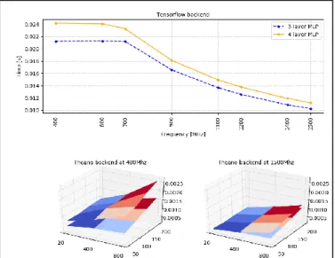
size (number of neurons). In Figure 1, the three dashed lines represent a neural network having hidden layer’s sizes of 20, 400 and 800 (the same holds for the straight lines). We notice a high difference in startup time: Theano backend is almost ten times slower to start than TensorFlow. The network size has also a greater impact with Theano.
Figure 1: Start-up time of the anomaly detector based on the MLP.
Regarding the prediction time, we notice that, using the TensorFlow backend, the network size and the window size have a negligible impact on the prediction time. This is not the case for the number of hidden layers and the CPU frequency, as depicted in the top graph in Figure 2. In the Theano tests instead, the prediction time (z-axes) is influenced by changing the window size (y-axes), the number of neurons in the hidden layer(s) (x-axes) and the frequency as depicted in the bottom graph in Figure 2. The time to make a prediction is also one order of magnitude smaller. However, in all cases, the prediction time stays below the threshold of 40 ms.
Figure 2: Time to make a prediction with the MLP architecture.
The results of memory consumption tests are summarized in Table I. From the test data, it appears that the memory consumption is clearly correlated with the network size with TensorFlow but not with Theano, which exhibits a higher and constant memory consumption.
TABLE I: MLP memory consumption.
Backend Layers Min [MB] Max [MB] Average [MB]
TensorFlow 3 289.087 298.072 292.173 TensorFlow 4 289.45 301.542 293.188 Theano 3 376.235 380.679 376.758 Theano 4 376.32 380.364 376.165
2) Long short-term memory network
Similarly to the MLP-based IDS, we tested the two following configurations:
3-layer LSTM: 1 input, 1 hidden layer, 1 output 4-layer LSTM: 1 input, 2 hidden layers, 1 output For both of them, the number of neurons in the input and output layer was set to 4. Here again, the difference between the Theano and Tensorflow backends is important. Similarly to the MLP case, Tensorflow is about five time faster to boot the IDS. Moreover, as expected, the LSTM architecture requires more time than the MLP due to the higher complexity in the LSTM network design. In Figure 3, the three overlapping dashed and straight lines represent different LSTM hidden layer(s) dimension (i.e., 5, 50 and 100 neurons). While the size of the hidden layer(s) plays a minor role (curves are overlapping), the addition of one layer causes an important increase in the start-up time, especially with the Theano backend.
Figure 3: Start-up time of the anomaly detector based on the LSTM.
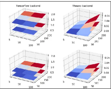
The graph below represents the time to make a prediction (z-axes) with the LSTM neural network in different conditions. We varied the number of hidden layers between 1 and 2, which are showed as two separated surfaces in the four 3D plots, where the top ones being logically the 4-layered LSTM. Also in this case, the tested hidden layer(s) dimension(s) were 5, 50 and 100 neurons (x-axes); for the window size the values were 50, 100, 150 and 200 (y-axes). In addition, we tested all the parameters combination for frequencies up to 1.5 GHz. In the Figure 4, we show only the results for the two “boundary” frequencies, i.e.
the CPU was set to 400MHz for the plots on the first row and 1500MHz for the ones in second row.
Figure 4: Time to make a prediction with the LSTM architecture.
The main result is that the prediction time (z-axis) is significantly higher with the TensorFlow backend, up to about 20 times if we compare the 3-layered cases at 1.5 Ghz, and systematically above 40ms. This means that the LSTM with the Tensorflow backend is not a good choice for the real-time IDS. It is also interesting to notice that, setting Theano as backend, the relative influence of the network size on the prediction time is much greater. On the other hand, we notice that the window size drives the prediction time with Tensorflow.
Regarding the peak of RAM usage for the LSTM neural network (Table II), it appears that the memory consumption is correlated with the network size using Tensorflow. Once again, this is not the case with Theano, which exhibited an almost constant memory consumption.
TABLE II: LSTM memory consumption
Backend Layers Min [MB] Max [MB] Average [MB]
Tensorflow 3 300.651 304.867 302.208 Tensorflow 4 307.086 313.179 309.928 Theano 3 376.597 380.609 377.03 Theano 4 376.534 380.179 376.836
D. Hyperparameters Optimization
In machine learning, there is no a common model architecture that fits to all problems, but rather each task has its own; it is often said that the problems are data-dependent. To this extent, we run a model selection algorithm to find the best set of hyper-parameters for both neural network architectures.
Given a model with a fixed hyper-parameter configuration, there are several approaches to evaluate its performance. We relied on k-fold cross validation, which was proven to be one of the best methods used for model selection [25]. We fixed the number of folds to 10, according to the recommendations of [25]. The configurations used for tests are characterized by six different parameters: number of neurons per layer, window size, hidden layers activation function, output layer activation function, weight initializer and the optimizer. For each of these
parameters, a range of possible values similarly to some related works. Some neural network configurations are explored manually to check whether the defined parameters ranges are appropriate for our data. Doing so, we could further shrink the domain size and thus increase the probability of finding the optimal parameter setting. The final grid of values is summarized below.
Hidden layer activation function = ['tanh', 'softsign', 'linear']
Output layer activation function = ['tanh', 'softsign', 'linear']
Weight initializer = ['lecun_uniform', 'glorot_normal', 'glorot_uniform', 'he_normal', 'he_uniform']
optimizer = ['Adagrad', 'Adam', 'Nadam', 'RMSprop'] Number of hidden layers’ neurons:
o 3 layer LSTM = [10,100]; 4 layer LSTM = [10,100] o 3 layer MLP = [10,800]; 4 layer MLP = [10,500] Window size = [5, 200]
Within this 6-dimensional configuration space, we decided to use random search to pick a value from each parameter grid, with uniform probability, and thus build a configuration to test. This decision is based on the work of Bergstra and Bengio [26], who proved its superior efficiency in comparison with gird and manual search.
In order to train and test a given neural network configuration, we need to set the number of epochs and the batch size. Following the practical recommendations for gradient-based training of deep architectures [27], the batch size should affect the training time and not so much the test performance. Hence, it can be optimized separately and after the other hyper-parameters. Therefore, in order to accelerate the optimization process, we kept the batch size fixed to 4096. Regarding the number of epochs, we applied early stopping; for each of the k times that train-test procedure is repeated for a given parameter setting, 20% of the training set (composed of k-1 folds) is reserved for validation phase. In order to prevent the leakage of test data information and therefore obtaining an unbiased performance estimate, we did not use the k-th fold, reserved for testing, also for validation.
Within the 10-fold validation process, at the end of each of the 10 training phases, the performance of the model has been assessed on the test fold in terms of Mean Squared Error (MSE). We run the hyper-parameter optimization procedure explained above on a custom computer equipped with an Nvidia GTX 1080 Ti GPU. We fixed the number of trials of the random search to 1000. In table III, we show for each configuration, the parameter settings having the smaller average mean square error.
TABLE III: Best configurations.
# Score Configuration
1 8.0949×10⁻⁴ MLP: HL = 2, AF & AFO = softsign, W = 49, WI =
glorot_uniform, O = Adam, N = 375
2 8.1998×10⁻⁴ MLP: HL = 1, AF & AFO = softsign, W = 38,
WI = glorot_normal, O = Adam, N = 599
3 8.2751×10⁻⁴ LSTM: HL = 1, AF = softsign, AFO = tanh, W = 79, WI =
he_uniform, O = Adam, N = 71
4 8.3355×10⁻⁴ LSTM: HL = 2, AF = softsign, AFO = tanh, W = 52,
a.
HL = hidden layers; AF = activation function; AFO = output activation function; W = window; WI = weight initializer; O = optimizer; N = number of neurons per layer
The above results show that the carefully selected architectures, in their best configurations, achieves performance similar to one another. According to the obtained results in Table III, we decided to base our IDS upon the MLP model bas on two reasons. First, it has the lowest average mean square error in the hyper-parameter optimization process. Second, it puts less strain on the underlying hardware infrastructure, which is more suitable for real time applications. Therefore, we trained the selected neural network for the last time using all the training samples and a batch size of 512, to obtain the final matrix of weights and biases.
We tested the trained neural network on the test set, set aside in the beginning, to see if the hyper-parameter optimization procedure yielded a configuration that was able to generalize well, without being under-fitted or over-fitted. Specifically, we computed the average of the mean square errors between predicted and real samples that resulted to be equal to 8.9225×10⁻⁴. As expected, the result was worse than the one
obtained in Table III but still has a high quality.
E. Anomaly Signal
As previously mentioned, we decided to use the squared distance as anomaly signal. We run the predictor on 50% of the test dataset samples, obtaining a forecast for each one of them. Then, we computed the squared error between each component of the predicted vector (𝑦̂) and its corresponding real value, part of the vector 𝑦. Then, we extrapolated the following information: average (avg), maximum and standard deviation (std) of the squared errors of each vector’s components (velocity, acceleration, longitude and latitude). These metrics have been used to compute different threshold values to be tested in the IDS (see subsection IV.E). Instead of one single metric, we decided to calculate a threshold for each predicted vector’s component. The finer granularity avoids that an anomaly on a single vector component could be compensated by the accurate prediction on the other components and thus pass without detection. An example is the MSE where, by averaging the squared errors of the different vector’s components, an anomaly could be “filtered out” and the resulting value could remain below the computed threshold.
IV. EXPERIMENTS AND RESULTS
Evaluating an IDS requires to compute the True Positive Rate (TPR) and False Positive Rate (FPR). These computations require a dataset containing normal and anomalous data. Unfortunately, the latter was not part of the available test dataset, so we turned to artificially injecting anomalies in the remaining 50% of it (~ 20k samples). Inspired by previous works [22], we devised three modifications that aim at emulating the characteristic of real in-vehicle networks attacks:
Drop. Four consecutive packets have a single value removed. This simulates what happens when an ECU is silenced and rapidly replaced by a malicious one. Fuzzing. Random data is introduced inside a sequence
in order to emulate a Denial of service (DoS) attack against the Controller Area Network (CAN) bus.
Discontinuity. The normal packet sequence is interleaved with a window of data taken from another point in time. This simulates a replay attack where an attacker takes control of an ECU and starts sending out of context, but legitimate traffic.
In addition, we needed to define the threshold value (THV) for each vector’s component and for how many (out of 4) squared errors above the threshold (THN) an alert should be raised. To do so, we carried out different experiments. We launched one attack at a time and varied:
THV in the range [avg + b × std, maximum] ∀ b ∈ [0, 1, 2, …, 6]
The attacked component between [acceleration, velocity, longitude, latitude].
NTH ∈ [2+, 3+, 4].
An anomaly detector in a vehicle should have a false alert as close as possible to zero. In the considered scenario, a false positive rate of 10−5 would produce a false alert almost every hour. This motivated us to choose an IDS’s setting that would lead to the highest possible TPR with a FPR of 0. The experiments results showed that the configuration that could achieve the aforementioned performances was the one with TH = (avg + 4 × std) and NTH = 3.
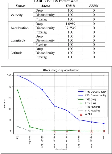
TABLE IV: IDS Performances.
Sensor Attack TPR % FPR% Velocity Drop 100 0 Discontinuity 100 0 Fuzzing 100 0 Acceleration Drop 1.0989 0 Discontinuity 37.2549 0 Fuzzing 100 0 Longitude Drop 100 0 Discontinuity 100 0 Fuzzing 100 0 Latitude Drop 100 0 Discontinuity 100 0 Fuzzing 100 0
From Table IV, we can notice a low detection rate of the discontinuity and drop attack against the acceleration. Figure 5 shows more details about the IDS behavior in case of attacks targeting the acceleration. It can be seen that it is possible to reach higher TPR values for all the attacks with the side effect of rising the FPR up to almost 10% (overlapping dashed lines).
V. CONCLUSION
In this paper, we presented a study on the usage of deep neural networks for anomaly detection in data sequences. In most of existing related works, the LSTM is the recommended model for time series problems. In our work we show that, in some cases, as previously discovered in [24], using a less complex neural network configuration, the MLP-based model can outperform the LSTM-based one. Moreover, we provided an extensive comparison of the real-time performances and hardware requirements of such a networks in a real-world implementation.
ACKNOWLEDGMENT
This work has received funding from the European Union Horizon 2020 research and innovation program as part of the VI-DAS project, under the grant agreement No 690772. The authors wish to thank the project partner Intempora for providing the RTMaps software and their technical support. We thank the TU/e Eindhoven for providing the driving data upon which this research has been carried out.
REFERENCES
[1] S. Tuohy, M. Glavin, C. Hughes, E. Jones, M. Trived, L. Kilmartin, “Intra-vehicle networks: A Review”, IEEE Transactions on Intelligent Transportation Systems, vol. 16, pp. 534-545, 2014.
[2] S. Biswas, R. Tatchikou, F. Dion, “Vehicle-to-vehicle wireless communication protocols for enhancing highway traffic safety”, IEEE Communications Society, vol. 44, pp. 74-82, 2006.
[3] M. Kissai, B. Monsuez, A. Tapus, “Current and future architectures for integrated vehicle dynamics control”, 2017.
[4] Karl Koscher et al., “Experimental security analysis of a modern automobile”, IEEE, 2010.
[5] C. Miller, C. Valasek, “Adventures in automotive networks and control units”, 2014.
[6] S. Checkoway et al., “Comprehensive experimental analyses of automotive attack surfaces”, USENIX Security, 2012.
[7] P. Kleberger, T. Olovsson, E. Jonsson, “Security aspects of the in-vehicle network in the connected car”, Intelligent Vehicles Symposium (IV), 2011 IEEE, 2011.
[8] V. Chandola, “Anomaly detection: a survey”, ACM Computing Surveys, vol. 41, article 15, 2009.
[9] E. Keogh et al., “Efficiently finding the most unusual time series subsequence”, ICDM '05 Proceedings of the Fifth IEEE International Conference on Data Mining, pp. 226-233, 2005.
[10] A. Nanduri, L. Sherry, “Anomaly detection in aircraft data using Recurrent Neural Networks”, Integrated Communications Navigation and Surveillance (ICNS), 2016.
[11] P. Filonov, A. Lavrentyev, A. Vorontsov, “Multivariate industrial time series with cyber-attack simulation: fault detection using an LSTM-based predictive data model”, arXiv:1612.06676, 2016.
[12] M. Yadav, P. Malhotra, L. Vig, K. Sriram, G. Shroff, “Augmented training improves anomaly detection in sensor data from machines”, NIPS Time-series Workshop, 2015.
[13] P. Malhotra, A. Ramakrishnan, G. Anand, L. Vig, P. Agarwal, G. Shroff, “LSTM-based encoder-decoder for multi-sensor anomaly detection”, ICML 2016 Anomaly Detection Workshop, 2016.
[14] I. Kiss, P. Haller, A. Bereş, “Denial of Service attack detection in case of tennessee eastman challenge process”, Procedia Technology, vol. 19, pp. 835-841, 2015.
[15] L. Chiang et al., “Fault detection and diagnosis in industrial systems”, Measurement Science and Technology, vol. 12, article 10, 2001. [16] L. Martí et al., “Anomaly detection based on sensor data in petroleum
industry applications”, Physical Sensors, 2015.
[17] D. Matteson, N. James, “A non-parametric approach for multiple change point analysis of multivariate data”, 2013.
[18] P. Malhotra, L. Vig, G. Shroff, P. Agarwal, “Long Short Term Memory Networks for anomaly detection in time series”, ESANN 2015 proceedings, 2015.
[19] S. Chauhan, L. Vig, “Anomaly detection in ECG time signals via deep long short-term memory networks”, Data Science and Advanced Analytics (DSAA), 2015.
[20] T. O'Shea, T. Clancy, R. McGwier, “Recurrent neural radio anomaly detection”, 2016.
[21] M. Kang, J. Kang , “Intrusion detection system using deep neural network for in-vehicle network security”, Plos One, 2016.
[22] A. Taylor, S. Leblanc, N. Japkowicz, “Anomaly detection in automobile control network data with long short-term memory networks”, Data Science and Advanced Analytics (DSAA), 2016.
[23] J. Moreno, A. Pol, P. Gracia, “Artificial neural networks applied to forecasting time series” , Psicothema, vol. 23, article 2, pp. 322-329, 2011. [24] F. Gers, D. Eck, J. Schmidhuber, “Applying LSTM to time series
predictable through time-window approaches”, 2002.
[25] Ron Kohavi, “A Study of cross-validation and bootstrap for accuracy estimation and model selection”, International Joint Conference on Artificial Intelligence (IJCAI), 1995.
[26] J. Bergstra, Y. Bengio, “Random search for hyper-parameter optimization”, JMLR, vol. 13, pp. 281-305, 2012.
[27] Y. Bengio, “Practical recommendations for gradient-based training of deep architectures”, Neural Networks: Tricks of the Trade, pp. 437-478, 2012.
[28] S. Bittl et al., “Performance comparison of data serialization schemes for ETSI ITS Car-to-X communication systems”, International Journal on Advanced Telecommunications, pp. 48-58.
[29] A. Singh, V. Tripathi, “Load Forecasting Using Multi-Layer Perceptron Neural Network”, IJESC, vol. 6, Issue no. 5, 2016.
[30] S. Canu, Y. Grandvalet, X. Ding, “One step ahead forecasting using multilayered perceptron”.