HAL Id: cea-01323613
https://hal-cea.archives-ouvertes.fr/cea-01323613
Submitted on 30 May 2016
HAL is a multi-disciplinary open access
archive for the deposit and dissemination of
sci-entific research documents, whether they are
pub-lished or not. The documents may come from
teaching and research institutions in France or
abroad, or from public or private research centers.
L’archive ouverte pluridisciplinaire HAL, est
destinée au dépôt et à la diffusion de documents
scientifiques de niveau recherche, publiés ou non,
émanant des établissements d’enseignement et de
recherche français ou étrangers, des laboratoires
publics ou privés.
Principal component analysis of event-by-event
fluctuations
Rajeev S. Bhalerao, Jean-Yves Ollitrault, Subrata Pal, Derek Teaney
To cite this version:
Rajeev S. Bhalerao, Jean-Yves Ollitrault, Subrata Pal, Derek Teaney. Principal component analysis
of event-by-event fluctuations. Physics Letters B, Elsevier, 2015, 114 (15), pp.2301.
�10.1103/Phys-RevLett.114.152301�. �cea-01323613�
Rajeev S. Bhalerao,1 Jean-Yves Ollitrault,2 Subrata Pal,3 and Derek Teaney4
1
Department of Theoretical Physics, Tata Institute of Fundamental Research, Homi Bhabha Road, Mumbai 400005, India
2CNRS, URA2306, IPhT, Institut de physique theorique de Saclay, F-91191 Gif-sur-Yvette, France
3
Department of Nuclear and Atomic Physics, Tata Institute of Fundamental Research, Homi Bhabha Road, Mumbai 400005, India
4Department of Physics and Astronomy, State University of New York, Stony Brook, NY 11794, USA
(Dated: April 1, 2015)
We apply principal component analysis to the study of event-by-event fluctuations in relativistic heavy-ion collisions. This method brings out all the information contained in two-particle correla-tions in a physically transparent way. We present a guide to the method, and apply it to multiplicity fluctuations and anisotropic flow, using ALICE data and simulated events. In particular, we study elliptic and triangular flow fluctuations as a function of transverse momentum and rapidity. This method reveals previously unknown subleading modes in both rapidity and transverse momentum for the momentum distribution as well as elliptic and triangular flows.
PACS numbers: 25.75.Ld, 24.10.Nz
I. INTRODUCTION
Anisotropic flow, vn, is one of the most striking
obser-vations in nucleus-nucleus collisions at ultrarelativistic energies [1, 2]. It is an azimuthal asymmetry of par-ticle production, which is interpreted as a signature of the system’s hydrodynamic response to the initial den-sity profile of the overlap zone of the colliding nuclei. The anisotropic flow thus provides a handle on the important issue of thermalization of the quark-gluon matter formed in these collisions. Event-by-event fluctuations of the ini-tial density profile have long been recognized to play a crucial role in the interpretation of elliptic flow v2 [3]
and they are solely responsible for triangular flow v3 [4].
However, the methods used to analyze anisotropic flow, namely the event-plane method [5] and cumulants [6], were devised before the importance of fluctuations was recognized. There are several discussions in the litera-ture of how the existing methods are affected by flow fluctuations [7–12].
We present a new method which unlike previous meth-ods extracts the flow fluctuations directly from data by fully exploiting all the information contained in two-particle correlations [13]. It also reveals an event-by-event substructure in flow fluctuations whose various components are organized by size thereby isolating the most important fluctuations. These can be systemati-cally analyzed by model calculations thus providing ad-ditional constraints on the initial-state dynamics.
The flow picture is that particles are emitted indepen-dently with an underlying probability distribution which varies event to event [14]. In each event we write the single-particle distribution with dp ≡ dptdη dϕ as
dN dp = +∞ X n=−∞ Vn(p)einϕ, (1)
where ϕ is the azimuthal angle of the outgoing particle momentum, Vn(p) is a complex Fourier flow coefficient
whose magnitude and phase fluctuate event to event, and p is a shorthand notation for the remaining momentum coordinates, pt and η. V0(p) is real and corresponds to
the momentum distribution, and Vn∗ = V−n. Note that
the usual definition of anisotropic flow vnis real and
nor-malized: vn = |Vn|/V0.
The covariance matrix of the flow harmonics Vn(p)
can be measured from the distribution of particle pairs. Specifically, in the flow picture the pair distribution is de-termined (predominantly) by the statistics of the event-by-event single particle distribution
dNpairs dp1dp2 = dN dp1 dN dp2 + O(N ), (2) where angular brackets denote an average over events, and the term O(N ) corresponds to correlations not due to flow (“nonflow”), which are small for large systems.
If the pair distribution is also expanded in a Fourier series dNpairs dp1dp2 = +∞ X n=−∞ Vn∆(p1, p2)ein(ϕ1−ϕ2), (3)
then the measured series coefficients Vn∆ are determined
by the statistics of Vn:
Vn∆(p1, p2) = hVn(p1)Vn∗(p2)i , (4)
where we have neglected nonflow correlations.1 The
right-hand side of Eq. (4) is a covariance matrix, hence it is positive semidefinite. Thus a nontrivial property of flow correlations is that the measured pair correlation matrix Vn∆(p1, p2) has only non-negative eigenvalues.2
1There is no systematic way of disentangling flow fluctuations and
nonflow, unless specific assumptions are made [15, 16].
2Back-to-back jets, on the other hand, typically result in large
negative diagonal elements for odd n [17], hence negative eigen-values.
2
The current Letter uses the eigenmodes and eigenval-ues of the two-particle correlation matrix, Vn∆(p1, p2),
to fully classify flow fluctuations in heavy-ion collisions. Specifically, we show how a Principal Component Anal-ysis (PCA) [18] of Vn∆(p1, p2) can be used to fully
ex-tract information on the pseudorapidity and transverse-momentum-dependence of flow fluctuations. We first test the applicability of the method with Monte-Carlo simulations using the transport model AMPT [19] in both rapidity and transverse-momentum. In addition to the leading eigenmode, corresponding to the usual anisotropic flow (for n > 0), the correlation analysis re-veals at least one important subleading mode in both rapidity and pt for the momentum distribution and its
second and third harmonics. Then we analyze ALICE data [13] in transverse-momentum and determine the first subleading elliptic and triangular flow coefficients.
II. METHOD
Divide the detector acceptance into Nb bins in
trans-verse momentum and/or pseudorapidity, p = (pt, η). The
sample estimate for Vn(p) in a given event (usually
re-ferred to as the flow vector [5]) is
Qn(p) ≡ 1 2π∆pt∆η M (p) X j=1 exp(inϕj), (5)
where M (p) is the number of particles in the bin and ϕj
is the azimuthal angle of a particle. The pair distribution is
Vn∆(p1, p2) ≡ hQn(p1)Q∗n(p2)i −
hM (p1)i δp1,p2
(2π∆pt∆η)2
− hQn(p1)i hQ∗n(p2)i , (6)
where the second term of the right-hand side subtracts self-correlations [20]. If self-correlations are not sub-tracted, Vn∆(p1, p2) is positive semidefinite by
construc-tion. After subtraction, eigenvalues may have both signs. However, the eigenvalues will be positive if the correla-tions are due to collective flow.
The last term on the right-hand side of Eq. (6) sub-tracts the mean value in order to single out the fluctua-tions. For n > 0 and an azimuthally symmetric detector, this term vanishes by azimuthal symmetry. For an asym-metric detector, subtracting the mean value corrects for azimuthal anisotropies in the acceptance [21, 22] Note that we define Vn∆(p1, p2) as a sum over all pairs, as
opposed to the usual normalization [4, 13] where one av-erages over pairs in each bin.3
3 The present normalization is required by the principal
compo-nent analysis for n = 0, and is desirable for n = 2, 3 because
The principal component analysis approximates the pair distribution as:
Vn∆(p1, p2) ≈ k
X
α=1
Vn(α)(p1)Vn(α)∗(p2), (7)
where each term in the sum corresponds to a different component (mode) of flow fluctuations, and k ≤ Nb.
If there are no flow fluctuations, the pair distribution Vn∆(p1, p2) factorizes [13] and there is only one
com-ponent, i.e. k = 1 in Eq. (7), corresponding to the usual anisotropic flow. Flow fluctuations break factoriza-tion [25]. Higher-order principal components then reveal information about the statistics and momentum depen-dence of flow fluctuations.
In practice, the principal components are obtained by diagonalizing Vn∆(p1, p2) = Pαλ(α)ψ(α)(p1)ψ(α)∗(p2)
(where ψ(α)(p) denotes the normalized eigenvector) and
ordering eigenvalues λ(α) from largest to smallest, λ(1) >
λ(2)> λ(3)· · · . Identifying with Eq. (7), one obtains
Vn(α)(p) ≡pλ(α)ψ(α)(p). (8)
Because of the square root, eigenvalues must be positive. If parity is conserved, the correlation matrix Vn∆(p1, p2)
is real up to statistical fluctuations, and Vn(α)(p) can be
chosen to be real.
The flow in a given event can be written as
Vn(p) = k
X
α=1
ξ(α)Vn(α)(p), (9)
where ξ(α) are complex, uncorrelated random variables
with zero mean and unit variance, that is, hξ(α)i = 0
and hξ(α)ξ(β)∗i = δ
α,β. The rms magnitude and
mo-mentum dependence of flow fluctuations are determined by the corresponding properties of the principal compo-nents. Since eigenmodes are real, the azimuthal angle of anisotropic flow in a specific event is solely determined by the phases of ξ(α).
For sake of compatibility with the usual definition of vn(p) which is the anisotropy per particle, we define
v(α)n (p) ≡ V
(α) n (p)
hV0(p)i
. (10)
Thus, v(α)0 (p) describe relative multiplicity fluctuations, while v(α)n (p) describe fluctuations of anisotropic flow.
it gives weight to a bin that is of the order of the number of particles in it. Note that a similar normalization is now used in cumulant analyses of anisotropic flow, where it is better to give all pairs (or generally multiplets) the same weight [22–24].
III. RESULTS
In order to illustrate the method, we analyze 104 Pb-Pb collisions at √s = 2.76 TeV in the 0-10% central-ity range,4generated using the string-melting version of
the AMPT model [19]. Initial conditions are generated via the HIJING 2.0 model [26] which contains nontrivial event-by-event fluctuations at the nucleonic and partonic levels [27]. In AMPT, collective flow is generated mainly as a result of partonic cascade. AMPT also has reso-nance formations and decays, and thus contains non-flow effects. We have checked that the present implementa-tion reproduces LHC data for anisotropic flow (v2 to v6)
at all centralities [28].
We first construct the pair distribution, Eq. (6), for all particles in the −3 < η < 3 pseudorapidity window, in η bins of 0.5. We then diagonalize the 12×12 matrix corre-sponding to these pseudorapidity bins. The eigenvalues are in general strongly ordered from largest to smallest. There are a few negative eigenvalues which can be at-tributed to statistical fluctuations.5
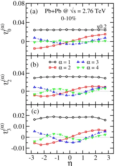
The leading principal components for n = 0, n = 2, and n = 3 are shown in Fig. 1. Fig. 1 (a) displays the principal modes of multiplicity fluctuations (n = 0) as a function of pseudorapidity. The leading mode v0(1)(η) is a global 12% relative fluctuation, independent of η, corresponding to the fluctuation of the total multiplic-ity within the event sample. The next-to-leading mode v0(2)(η) is odd and of much smaller amplitude, as shown by the eigenvalues, λ(2) ∼ λ(1)/60. A natural source of
this odd mode is the small difference between the partic-ipant numbers of projectile and target nuclei induced by fluctuations, which creates a forward-backward asymme-try of the multiplicity [29, 30]. Since both the colliding system and the analysis window are symmetric around η = 0, principal components have definite parity in η, up to statistical fluctuations. Indeed, the next mode v0(3)(η) is even, suggesting that principal components typically have alternating parities. The corresponding eigenvalue is again much smaller, λ(3) ∼ λ(2)/5. v(4)
0 (η) and higher
modes are blurred by statistical fluctuations. Note that Eq. (7) defines principal components up to a sign. Here, we conventionally choose vn(α)(η) > 0 at forward
rapid-ity. Fig. 1 also illustrates the orthogonality of principal components, that is,
X
η
Vn(α)(η)Vn(β)∗(η) = 0 if α 6= β. (11)
4 We only show one centrality bin for sake of illustration, but we
have checked that results are similar for other centralities.
5 This can be checked by applying the PCA to purely
statisti-cal fluctuations. We generated random matrices according to the statistical error of Vn∆(p1, p2), and found that the
nega-tive eigenvalues of Vn∆(p1, p2) are compatible with the negative
eigenvalues of these random matrices.
0
0.04
0.08
v
0
(α
)
0
0.04
v
2
(α
)
α = 1
α = 2
-3
-2
-1
0
1
2
3
η
-0.01
0
0.01
0.02
v
3
(α
)
α = 3
α = 4
Pb+Pb @ √s = 2.76 TeV
0-10%
x0.2
(a)
(b)
(c)
FIG. 1. Principal component analysis as a function of
pseu-dorapidity for Pb+Pb collisions at√s = 2.76 TeV in the
0-10% centrality window generated with AMPT. (a) Multiplic-ity fluctuations; (b) Elliptic flow fluctuations; (c) Triangular flow fluctuations.
Thus, v(α)n (η) typically has α − 1 nodes.
Fig. 1 (b) and (c) display the principal components of elliptic and triangular flow fluctuations as a function of pseudorapidity. The leading modes v(1)n (η) correspond
to the usual elliptic and triangular flows, which depend weakly on η at the LHC [31, 32]. The subleading modes v(2)n (η) are odd and of smaller amplitude (λ(2)' λ(1)/13).
These rapidity-odd harmonic flows, or torqued flows, can be attributed to the small relative angle between n-th harmonic participant planes defined in the projectile and target nuclei [33].
Note that the correlation matrix Vn∆(η1, η2) is the sum
of flow and nonflow correlations [34]. The nonflow corre-lation is significant only for small values of the relative pseudorapidity ∆η ≡ |η1− η2|. If the range in ∆η is
smaller than the binning, it contributes to the diagonal elements, and its effect is to shift all eigenvalues by a con-stant. We observe in general a clear ordering of eigenval-ues (λ(2)/λ(3) ∼ λ(3)/λ(4) ∼ 2) which suggests that the
4
correlation has a long range in ∆η and is therefore dom-inated by flow. Visual inspection of correlation matrix Vn∆(η1, η2) qualitatively confirms this reasoning.
We then carry out the analysis as a function of trans-verse momentum. In addition to AMPT generated events, we use experimental data for Vn∆(p1, p2) provided
by the ALICE collaboration [13] for Pb+Pb collisions in the 0-10% centrality window. ALICE uses all charged particles in the pseudorapidity window |η| < 1. The def-inition of Vn∆ is not quite the same as ours: First, it is
averaged (as opposed to summed) over pairs. We correct for this difference by multiplying off-diagonal elements of Vn∆of ALICE by the average multiplicity of pairs in each
(p1, p2) bin, which we estimate using the statistical errors
provided by ALICE (σ ' (2Npairs)−1/2). The diagonal
elements are multiplied by twice the average multiplicity of the pairs, to account for self-correlations. Second, the analysis is done with a rapidity gap to suppress nonflow correlations: this means that particles 1 and 2 in Eq. (6) are separated by a rapidity gap of 0.8. For sake of com-parison, we repeat the analysis using AMPT events (the same as in Fig. 1). In order to compensate for the lower statistics, we use a wider pseudorapidity window, from −2 to 2, with a 0.8 rapidity gap between −0.4 and 0.4.
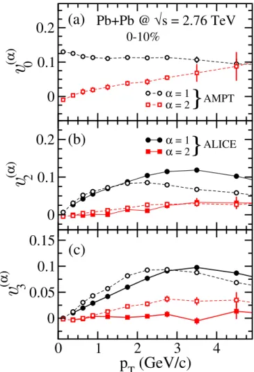
Fig. 2 (a) displays the two principal modes of multi-plicity fluctuations (n = 0) as a function of transverse momentum. Since no experimental data are available for this analysis, we only use AMPT events. As in Fig. 1 (a), the leading mode is essentially constant and corre-sponds to the 12% fluctuation in the total multiplicity. The subleading mode increases linearly as a function of pt for large pt, which can be interpreted as the result
of a radial flow fluctuation. Specifically, in a hydrody-namic model the number of particles at high ptdecreases
as, exp (pt(u − u0)/T ), where u is the maximum fluid
4-velocity, u0=
√
1 + u2 and T is the temperature [35]. A
small variation in u therefore produces a relative varia-tion in the yield increasing linearly with pt.
Fig. 2 (b) and (c) display the two leading principal components for elliptic and triangular flows. ALICE data show a very strong ordering between the two leading eigenvalues (λ(1)/λ(2) ∼ 400 for n = 2, 300 for n = 3).
The leading components for n = 2 and n = 3 are very close to the value of v2 and v3 obtained using the same
data [13]. The subleading mode is of much smaller mag-nitude and becomes significant only at large transverse momentum. In a hydrodynamical model, such a behavior is expected. Indeed, in a typical event the phase angle of the harmonic flow at high-momentum deviates slightly from the phase angle at low-momentum [17, 37]. Thus, the flow of high-ptparticles has a small component
inde-pendent of the flow of low-pt particles. The subleading
mode determines the magnitude of this additional com-ponent. As we shall see below, it is also responsible for the factorization breaking of azimuthal correlations ob-served in these data [13, 25].
0
0.1
0.2
v
0
(α
)
α = 1 α = 20
0.1
0.2
v
2
(α
)
α = 1 α = 20
1
2
3
4
p
T
(GeV/c)
0
0.05
0.1
0.15
v
3
(α
)
Pb+Pb @ √s = 2.76 TeV
}
}
AMPTALICE
0-10%
(a)
(b)
(c)
FIG. 2. Principal component analysis as a function of
trans-verse momentum for Pb+Pb collisions at √s = 2.76 TeV
in the 0-10% centrality window, using ALICE data [13] (full symbols) and AMPT events (open symbols). (a) Multiplicity fluctuations; (b) Elliptic flow fluctuations; (c) Triangular flow fluctuations.
IV. DISCUSSION
This new method, unlike traditional analysis methods, makes use of all the information contained in two-particle azimuthal correlations. Specifically, it uses the detailed information on how they depend on the momenta of both particles, as opposed to traditional analyses which inte-grate over one of the momenta.
Previously, this double-differential structure has been used to test the factorization of azimuthal correlations. Small factorization breaking effects have been seen exper-imentally [13, 36] and in event-by-event hydrodynamic calculations [25, 37, 38]. They have been characterized by the Pearson correlation coefficient between two differ-ent momdiffer-enta:
r = Vn∆(p1, p2) pVn∆(p1, p1)Vn∆(p2, p2)
. (12)
correlations are due to flow.
These results are easily recovered in the language of principal components, in a physically transparent way. Factorization is the limiting case of just one principal component (k = 1 in Eq. (7)). In the more general case k > 1, Eq. (7) guarantees |r| ≤ 1: Cauchy-Schwarz in-equalities [25] are equivalent to the condition that all eigenvalues of the matrix Vn∆ are positive. Flow
fluc-tuations are typically dominated by a single subleading mode, i.e., k = 2, with |Vn(2)(p)| |Vn(1)(p)|. In this
limit, Eq. (12) gives
1 − r ' 1 2 Vn(2)(p1) Vn(1)(p1) −V (2) n (p2) Vn(1)(p2) 2 . (13)
We see that r ≤ 1 as required by the Cauchy-Schwarz inequality. Further, we see that the breaking of factor-ization is induced by the relative difference between the subleading mode and the leading mode.
To summarize, we have presented a new method to analyze the anisotropic flow data in relativistic heavy-ion collisheavy-ions. It is based on the Principal Component
Analysis applied to the two-particle correlation matrix. The principal components express the detailed informa-tion contained in correlainforma-tions in a convenient way, which can be directly compared with model calculations. The method has revealed for the first time subleading modes in both rapidity and pt in the harmonic coefficients for
n = 0, 2 and 3. We anticipate a rich experimental and theoretical program studying the dynamics of these sub-leading flow vectors, which can be used to further con-strain the plasma response to the initial geometry.
ACKNOWLEDGMENTS
We thank A. Bzdak for early discussions of this work. This work is funded by CEFIPRA under project 4404-2. JYO thanks the MIT LNS for hospitality, and acknowl-edges support by the European Research Council under the Advanced Investigator Grant ERC-AD-267258. DT is supported by the U.S. Department of Energy grant DE-FG02-08ER4154.
[1] U. Heinz and R. Snellings, Ann. Rev. Nucl. Part. Sci. 63, 123 (2013) [arXiv:1301.2826 [nucl-th]].
[2] C. Gale, S. Jeon and B. Schenke, Int. J. Mod. Phys. A 28, 1340011 (2013) [arXiv:1301.5893 [nucl-th]].
[3] B. Alver et al. [PHOBOS Collaboration], Phys. Rev. Lett. 98, 242302 (2007) [nucl-ex/0610037].
[4] B. Alver and G. Roland, Phys. Rev. C 81, 054905 (2010) [Erratum-ibid. C 82, 039903 (2010)] [arXiv:1003.0194 [nucl-th]].
[5] A. M. Poskanzer and S. A. Voloshin, Phys. Rev. C 58, 1671 (1998) [nucl-ex/9805001].
[6] N. Borghini, P. M. Dinh and J. Y. Ollitrault, Phys. Rev. C 64, 054901 (2001) [nucl-th/0105040].
[7] C. Adler et al. [STAR Collaboration], Phys. Rev. C 66, 034904 (2002) [nucl-ex/0206001].
[8] J. Adams et al. [STAR Collaboration], Phys. Rev. C 72, 014904 (2005) [nucl-ex/0409033].
[9] B. Alver, B. B. Back, M. D. Baker, M. Ballintijn, D. S. Barton, R. R. Betts, R. Bindel and W. Busza et al., Phys. Rev. C 77, 014906 (2008) [arXiv:0711.3724 [nucl-ex]].
[10] J. Y. Ollitrault, A. M. Poskanzer and S. A. Voloshin, Phys. Rev. C 80, 014904 (2009) [arXiv:0904.2315 [nucl-ex]].
[11] C. Gombeaud and J. Y. Ollitrault, Phys. Rev. C 81, 014901 (2010) [arXiv:0907.4664 [nucl-th]].
[12] M. Luzum and J. Y. Ollitrault, Phys. Rev. C 87, no. 4, 044907 (2013) [arXiv:1209.2323 [nucl-ex]].
[13] K. Aamodt et al. [ALICE Collaboration], Phys. Lett. B 708, 249 (2012) [arXiv:1109.2501 [nucl-ex]].
[14] M. Luzum, J. Phys. G 38, 124026 (2011)
[arXiv:1107.0592 [nucl-th]].
[15] M. Luzum, Phys. Lett. B 696, 499 (2011)
[arXiv:1011.5773 [nucl-th]].
[16] L. Xu, L. Yi, D. Kikola, J. Konzer, F. Wang and W. Xie,
Phys. Rev. C 86, 024910 (2012) [arXiv:1204.2815 [nucl-ex]].
[17] J. Y. Ollitrault and F. G. Gardim, Nucl. Phys. A 904-905, 75c (2013) [arXiv:1210.8345 [nucl-th]].
[18] I. Jolliffe, Principal component analysis, in Encyclopedia of statistics in behavioral science, Wiley Online Library (2005).
[19] Z. W. Lin, C. M. Ko, B. A. Li, B. Zhang and S. Pal, Phys. Rev. C 72, 064901 (2005) [nucl-th/0411110]. [20] P. Danielewicz and G. Odyniec, Phys. Lett. B 157, 146
(1985).
[21] N. Borghini, P. M. Dinh and J. Y. Ollitrault, Phys. Rev. C 63, 054906 (2001) [nucl-th/0007063].
[22] A. Bilandzic, C. H. Christensen, K. Gulbrandsen,
A. Hansen and Y. Zhou, Phys. Rev. C 89, no. 6, 064904 (2014) [arXiv:1312.3572 [nucl-ex]].
[23] R. S. Bhalerao, N. Borghini and J. Y. Ollitrault, Nucl. Phys. A 727, 373 (2003) [nucl-th/0310016].
[24] A. Bilandzic, R. Snellings and S. Voloshin, Phys. Rev. C 83, 044913 (2011) [arXiv:1010.0233 [nucl-ex]].
[25] F. G. Gardim, F. Grassi, M. Luzum and J. Y. Ollitrault, Phys. Rev. C 87, no. 3, 031901 (2013) [arXiv:1211.0989 [nucl-th]].
[26] W. T. Deng, X. N. Wang and R. Xu, Phys. Rev. C 83, 014915 (2011) [arXiv:1008.1841 [hep-ph]].
[27] L. Pang, Q. Wang and X. N. Wang, Phys. Rev. C 86, 024911 (2012) [arXiv:1205.5019 [nucl-th]].
[28] S. Pal and M. Bleicher, Phys. Lett. B 709, 82 (2012) [arXiv:1201.2546 [nucl-th]].
[29] A. Bzdak and D. Teaney, Phys. Rev. C 87, no. 2, 024906 (2013) [arXiv:1210.1965 [nucl-th]].
[30] V. Vovchenko, D. Anchishkin and L. P. Csernai, Phys. Rev. C 88, no. 1, 014901 (2013) [arXiv:1306.5208 [nucl-th]].
6
330 (2012) [arXiv:1108.6018 [hep-ex]].
[32] S. Chatrchyan et al. [CMS Collaboration], Phys. Rev. C 89, no. 4, 044906 (2014) [arXiv:1310.8651 [nucl-ex]]. [33] P. Bozek, W. Broniowski and J. Moreira, Phys. Rev. C
83, 034911 (2011) [arXiv:1011.3354 [nucl-th]].
[34] B. Alver et al. [PHOBOS Collaboration], Phys. Rev. C 81, 034915 (2010) [arXiv:1002.0534 [nucl-ex]].
[35] N. Borghini and J. Y. Ollitrault, Phys. Lett. B 642, 227
(2006) [nucl-th/0506045].
[36] CMS Collaboration [CMS Collaboration], CMS-PAS-HIN-14-012.
[37] U. Heinz, Z. Qiu and C. Shen, Phys. Rev. C 87, no. 3, 034913 (2013) [arXiv:1302.3535 [nucl-th]].
[38] I. Kozlov, M. Luzum, G. Denicol, S. Jeon and C. Gale, arXiv:1405.3976 [nucl-th].