Twelve quick tips for designing sound dynamical models for bioprocesses

HAL Id: hal-02421763

https://hal.inria.fr/hal-02421763

Submitted on 20 Dec 2019

HAL is a multi-disciplinary open access

archive for the deposit and dissemination of sci-entific research documents, whether they are pub-lished or not. The documents may come from teaching and research institutions in France or abroad, or from public or private research centers.

L’archive ouverte pluridisciplinaire HAL, est destinée au dépôt et à la diffusion de documents scientifiques de niveau recherche, publiés ou non, émanant des établissements d’enseignement et de recherche français ou étrangers, des laboratoires publics ou privés.

Twelve quick tips for designing sound dynamical models

for bioprocesses

Francis Mairet, Olivier Bernard

To cite this version:

Francis Mairet, Olivier Bernard. Twelve quick tips for designing sound dynamical models for bio-processes. PLoS Computational Biology, Public Library of Science, 2019, 15 (8), pp.e1007222. �10.1371/journal.pcbi.1007222�. �hal-02421763�

Twelve quick tips for designing sound dynamical models for

bioprocesses

Francis MAIRET1, Olivier BERNARD2,3,4,*,

1 Ifremer, Physiology and Biotechnology of Algae laboratory, rue de l’Ile d’Yeu, 44311 Nantes, France

2 Cˆote d’Azur University, INRIA, BIOCORE, BP93, 06902 Sophia-Antipolis Cedex, France

3 Sorbonne University, CNRS, LOV, 06230 Villefranche-sur-mer, France

4 ENERSENSE, Department of Energy and Process Engineering, NTNU, 7491 Trondheim, Norway

* olivier.bernard@inria.fr

Because of the inherent complexity of bioprocesses, mathematical models are more and 1

more used for process design, control and optimization etc... These models are generally 2

based on a set of biochemical reactions. Model equations are then derived from mass balance, 3

coupled to empirical kinetics. Biological models are nonlinear and represent processes, 4

which by essence are dynamic and adaptive. The temptation to embed most of the biology 5

is high, with the risk that calibration would not be significant anymore. The most important 6

task for a modeler is thus to ensure a balance between model complexity and ease of use. 7

Since a model should be tailored to the objectives which will depend on applications and 8

environment, a universal model representing any possible situation is probably not the best 9

option. 10

Here are twelve tips to develop your own bioprocess model. For more details on bioprocess 11

modelling, the readers could refer to [1]. More tips concerning computational aspects can 12

Tip 1: Define your objective and the application context

Years of high school learning about how to set-up mechanistic models based on the funda- 15

mental F = m.a relationship of mechanics, or on the Ohm law have corrupted our minds. 16

It took centuries to identify the corpus of laws supporting today’s physical models. Fig 17

1 recalls that, previously, there used to be some ”less accurate” predictive models that 18

have been forgotten. At present, models in these fields, even if empirical, are excellent 19

approximations and -at least for those we studied at school- always ended-up in rather 20

simple, often linear and mathematically tractable models. The complexity of biological 21

systems requires a more open viewpoint, where different models of the same process can 22

be useful and complementary. Therefore, before writing equations, one must first clearly 23

define the model objective. The model can be designed for numerous reasons, among 24

which prediction of future evolution, understanding of the process behaviour, estimation 25

of unmeasured variables or fluxes, operator training, detection and diagnosis of failures, 26

optimization and control. 27

Tip 2: Adapt your modelling framework with your objective,

your knowledge and your data set

When developing a model, it is crucial to keep in mind the objectives of the model and 30

the framework for its application. A model targeting the understanding of some metabolic 31

processes inherently requires the user to embark on the details of the cell metabolism [5, 6]. 32

Predicting the impact of meteorology on outdoor microalgal processes means that light 33

and temperature must be included somewhere in the model. A model for on-line control 34

can be more straightforward (often because it will benefit from on-line information on 35

process state). So, keeping in mind the model objective, one has to choose which variables 36

to include, but also the type of model: deterministic versus stochastic, homogeneous versus 37

heterogeneous (in terms of space or phenotype). The available data set or data that can 38

Fig. 1. Medieval theory of the canon ball trajectory, from Walther Hermann Ryff (1547) [4]. The canon ball trajectory was an assemblage of circular arcs and segments.

Models in physics are now excellent approximations, but they have sometimes been improved during century-long periods. In biology, we are still at the dawn of model development.

Parameters should be calibrated at some point, or at least reasonably determined from 40

the experimental information. Model complexity can first be measured by the number of 41

state variables (variables with dynamics) together with the number of parameters and stay 42

compatible with the objectives and data. 43

Tip 3: Take care with dimensions, intensive and extensive

properties

This tip seems very basic, but, in our opinion, it is worth emphasising. The dimension of 46

the model equation should be checked. Particular care should be taken between intensive 47

and extensive variables [7]. This is particularly true when dealing with a metabolic model. 48

A metabolite concentration could be expressed per unit of culture volume or intracellular 49

or by cellular growth, respectively. Moreover, the kinetics of intracellular reactions should 51

depend on intracellular concentrations, not culture concentrations. In several studies, it 52

remains unclear. 53

Tip 4: Do not assume gas concentrations equilibrate with

atmosphere

Assuming gas concentrations equilibrate with the atmosphere is a common mistake. If 56

we measure the dissolved CO2 concentration in a glass of water in equilibrium with the 57

atmosphere, it will be proportional to PCO2, the CO2 partial pressure at the interface (i.e. 58

in the air): [CO2] = KhPCO2 where Kh is Henry’s constant at the considered temperature 59

and salinity. At steady state, there is no more gas exchange between the atmosphere and 60

liquid phase. 61

If algae are developing in the glass, the CO2 concentration will be lower, because the

algae permanently consume it. As a consequence, there is a permanent flux of CO2 from

air to water, with a flow rate

QCO2 = KLa(CO2− KhPCO2)

which will balance the consumption of CO2 by the algae. Now the concentration of CO2 is 62

lower than KhPCO2, its natural equilibrium value without algae. 63

Tip 5: Check the mathematical soundness of your model

A mathematical analysis of your model may help to detect potential errors, limitations and 65

drawbacks in model design, and to better apprehend the process. Whenever possible, one 66

should check mass conservations, check the boundedness of the variables (in particular their 67

positivity), and study the asymptotic behaviour of the model. This last point could be, 68

for some models, particularly challenging. It is essential to keep in mind that nonlinear 69

including limit cycles, chaos or abrupt change in behaviours after bifurcation when one 71

of the model parameters has been slightly modified [8]. Mathematicians spend months 72

trying to understand and prove the behaviour of systems of low dimension, e.g. with ”only” 73

three state variables. The mathematical complexity is breath-taking when considering 74

standard bioprocess models. Often, the properties of these models are hardly suspected, 75

and Pandora’s box stays closed. Even the number of equilibria that can be produced is 76

rarely discussed. Adding new features or including more realism into a model extends the 77

risk of unexpected model behaviours. 78

The objective is to determine whether the trajectories of your system converge towards an 79

equilibrium (a global equilibrium, or different equilibria depending on the initial conditions), 80

if they present sustained oscillations (limit cycle) or even show a chaotic behaviour. These 81

properties should be in line with the behaviour of your bioprocess, otherwise the model 82

should be revised. 83

Tip 6: Be aware of structural identifiability

Most of the parameters in physical modelling have a clear meaning and can be directly 85

measured on the process. Also, physical models are often linear. The theory of linear 86

systems and their identification has received much attention, indirect identification of a 87

tenth of parameters can be accurately carried out by modern algorithms [9, 10]. For the 88

biological systems, which are in turn nonlinear and described by rough approximations, 89

more modesty is required. 90

Theoretical identifiability of the parameters is a complex mathematical property [11], 91

which is often characterized by cryptic (but accurate) mathematical formulations. In a 92

nutshell, this theoretical mathematical property states that a parameter value can be 93

uniquely determined by (nonlinear) combinations of measurements and their derivatives 94

(with respect to time) at any order. More simply, a unique set of parameters can produce a 95

given model output. With non-linear models, it is possible that two sets of parameters can 96

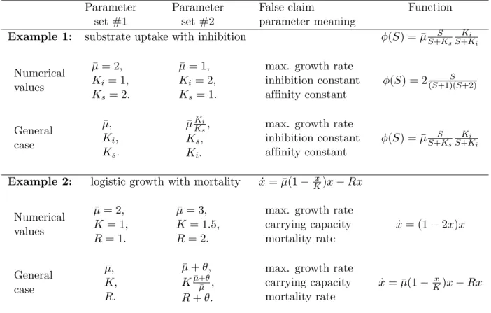
in Table 1 two illustrative astonishing examples for trivial models. 98

The first example is unfortunately not so rare. It consists in representing an inhibition 99

kinetics (from substrate S) with a product of Monod and a hyperbolic inhibition term. A 100

numerical example is given in Table 1 (Example 1), where two parameter sets produce 101

exactly the same values. Parameters here are only locally structurally identifiable. 102

The second example in Table 1 uses a trivial logistic equation (x is the biomass) modified 103

to deal with mortality rate (which is obviously a very bad idea). Here, an infinity of 104

parameters provide the same biomass dynamics, they are structurally not identifiable. 105

These two examples also demonstrate that it is useless to attribute a biological meaning 106

to a non-identifiable parameter. In the first case, what was, in turn, the inhibition constant: 107

Ki or Ks? In the second example, is K the carrying capacity of the medium? 108

Perhaps more problematic when using an automatic algorithm for parameter identifica- 109

tion, non-identifiable parameters will kill any approach. Especially if it is a global approach, 110

any optimisation algorithm will oscillate between several of the possible solutions, or average 111

them, and often will never converge. 112

In general, assessing identifiability for complex dynamical models is very challenging. 113

This is a reason why modellers must refrain from embedding too many processes into a 114

model, and privilege lower complexity models when only a limited set of measurements is 115

available for validation. 116

Tip 7: Double check numerical implementation

If your model has been implemented only once, then it probably contains at least three 118

mistakes. We know this is not true for you, but it is for most of the people. So if the model 119

was right, after a rapid change in one of the equations for testing the effect of one factor, it 120

would become wrong because eventually the test is not removed. There are strict coding 121

rules and use of validation tests [12], but they are rarely respected for model development 122

because the model implementation is generally not carried out by computer scientists. Also, 123

Table 1. Analysis of two simple examples with identifiability issues.

Parameter Parameter False claim Function set #1 set #2 parameter meaning

Example 1: substrate uptake with inhibition φ(S) = ¯µ_S+KS

s Ki S+Ki Numerical values ¯ µ = 2, Ki= 1, Ks= 2. ¯ µ = 1, Ki = 2, Ks= 1.

max. growth rate inhibition constant affinity constant φ(S) = 2_(S+1)(S+2)S General case ¯ µ, Ki, Ks. ¯ µKi Ks, Ks, Ki.

max. growth rate inhibition constant affinity constant φ(S) = ¯µ_S+KS s Ki S+Ki

Example 2: logistic growth with mortality x = ¯˙ µ(1 −_Kx)x − Rx

Numerical values ¯ µ = 2, K = 1, R = 1. ¯ µ = 3, K = 1.5, R = 2.

max. growth rate carrying capacity mortality rate ˙ x = (1 − 2x)x General case ¯ µ, K, R. ¯ µ + θ, Kµ+θ¯_µ¯ , R + θ.

max. growth rate carrying capacity mortality rate

˙

x = ¯µ(1 −_Kx)x − Rx

In Example 1, two different parameter sets produce the same value of the function φ(S). In Example 2, an infinite number of parameter sets can produce the same dynamics ˙x for an arbitrary value of θ. The parameters meaning (as often claimed) does then not make any sense.

more difficult to cross check. Excel® is an excellent tool for displaying data and for simple 125

computations, but it is not an appropriate tool for simulating complex models since it is 126

almost impossible to cross-check implementation. Some graphical languages also have these 127

drawbacks when a connection to a wrong node can corrupt the result while being almost 128

impossible to detect. 129

One way of reducing the risk of error is a double implementation, with two different 130

computer programmers and two different languages. This has been the case for the models 131

used in wastewater treatment, ADM1 for anaerobic digestion [13] and ASM1 for activated 132

sludge [14]. The first comparison between different implementations revealed to be quite 133

quaint. Also, simple case studies must help to check simple theoretical properties (positivity 134

of variables, mass conservation, etc...) that must be respected. 135

Tip 8: Pay attention to practical identifiability

The cost criterion to be optimised (typically the sum of squared errors) is generally non- 137

convex, and many local minima perturb parameter identification. In practice, it is often 138

not possible to get an accurate estimate of parameters from the data sets. The most 139

efficient algorithms are generally limited to three parameters to be determined per measured 140

quantity (assuming a reasonable sampling over time). The weird consequence is that fitting 141

a model to a set of data is generally possible, but that does not mean that the estimated 142

parameters are reasonable. Whenever a parameter has a clear meaning, the validity of the 143

identified value must always be checked, and bounds can be added during the identification 144

process. Multiple algorithm initialisations are also strongly recommended. Collecting 145

informative data is also key for practical identifiability, which means data corresponding 146

to high sensitivities of the model outputs with respect to parameter variations (cf. Fisher 147

information matrix [9]). As a matter of illustration, it is not possible to estimate a parameter 148

related to growth inhibition if substrate concentration is always too low to trigger inhibition. 149

Finally, a literature review is an essential resource for parameter values, in particular 150

parameters from different papers! 152

Tip 9: apply the ”divide and conquer” strategy to identify

your parameters

Do not try to get all your parameters at once, through a never converging optimization 155

algorithm and rather identify subsets of parameters. In many cases, after simple algebraic 156

manipulations some parts of the model can lead to relationships between some measured 157

quantities and eventually provide some combinations of the parameters. For example, the 158

pseudo-stoichiometry can often be identified independently of the reaction rates after some 159

straightforward transformations [15]. Some working modes do considerably simplify the 160

model, and are often an opportunity to extract such relationships. For example, during a 161

phase when nutrients are nonlimiting, the Michaelis-Menten kinetics can be replaced by 162

constants. Similarly, if different equilibria can be observed for various inputs, they would 163

probably lead to very interesting relationships between some of the model parameters [16]. 164

Tip 10: determine parameter and model uncertainties

Assessing measurement uncertainty propagation is of utmost importance to assess model 166

accuracy. This first means that the experimental data must be associated to the variance of 167

their measurement error. There are different strategies to compute not only the parameter 168

values but also their confidence intervals. This is straightforward when parameters are 169

deduced from linear relationship, but is can also be estimated in a more complex case 170

thanks to the covariance matrix of parametric errors [9]. The strong scientific added value 171

is that the simulation scheme will predict not only outputs but also the confidence intervals 172

Tip 11: Validate the model with data not used for identifica-

tion

When observing the vast diversity in bioprocess models, only a few of them have been 176

appropriately validated. First, because it is not possible to validate a model, a model 177

can only be discarded when it is not compliant with experimental records [17]. However, 178

assuming a relaxed use of the ”validation” term, it would mean that the model has been 179

proven accurate for a large variety of cases. In particular for cases significantly different 180

from the learning data set (data that has been used for the calibration). This ideal situation 181

is very difficult to meet in practice, and most of the time the validation datasets only differ 182

by some initial conditions, or by a single different forcing variable. If the model has enough 183

parameters, it can probably fit a calibration dataset nicely with only a few points. However, 184

it will exhibit abysmal performances for cross-validation. For larger calibration data sets, 185

the fit will probably less successfully highlight the quality of the model, but prediction 186

capacity might be highly enhanced. The plot will not look that nice, but the model will 187

definitely be more powerful and relevant. 188

Claiming that the model is valid is, therefore, an act of faith, and a very weak scientific 189

assertion. As running experiments takes time and is money consuming, the number of 190

experiments is by essence limited. As consequence, it becomes clear that the conditions for 191

which the model has been validated must be clearly stated. Knowing the ”model validation 192

domain” will in itself be precious for future model use. Also, providing data sets for which 193

the model did not do its job is intrinsically useful, although rarely done. 194

Often, the question is instead to choose the best model among a few candidates. A more 195

complex model, with more parameters, will mechanically better fit the data. However, that 196

does not mean it is more correct, it just means it is more flexible. The Akaike criterion [18] 197

is a good option to compare the performance of two models of different levels of complexity. 198

However, the only real criterion to assess the predictive power of a model, and therefore 199

to compare model performances is cross-validation, assessing the model with data which 200

the calibration data set). Additionally, the candidate models can even be used to find the 202

experimental conditions that will allow to differentiate them better [17]. 203

Finally, models can include the effects of different factors which often have been studied 204

separately. The models then gather these effects classically by multiplying the different 205

terms or using Liebig’s law of minimum. Validation experiments could be the last chance 206

to test possible interactions between these factors and find the best way to combine their 207

effects in the model. 208

Tip 12: Share codes, tips, tools, and model limitations

More and more journals require this, and it is to be welcomed. Providing your model - with 210

all the files necessary to reproduce your simulations (including parameter values, initial 211

conditions etc...) - will favour its dissemination within the scientific community. Your 212

model would thus be further validated with new data sets. Additionally, it promotes error 213

checking, helps the reader if some model details in the manuscript are unclear, and removes 214

any suspicion of fraud. 215

More generally, what makes the success and the efficiency of a model, is not limited to 216

the biology it embeds and to the realism of its predictions. A model is inexorably associated 217

with a set of tools to calibrate it, estimate which are the most sensitive parameters, optimise 218

a criterion, determine the input which maximizes productivity etc... The associated toolbox 219

to make the model applicable and efficient is probably at least as necessary as the model 220

itself. Great models can have complex structures or behaviours, which eventually make 221

their use more tricky. For example, the outstanding Geider model [19] is in turn rather 222

challenging to calibrate, and specific methods dedicated to its calibration are needed [20]. 223

Even simpler models, such as the Hinshelwood model [21] for temperature, advantageously 224

predicts a mortality rate [22], but calibrating this model often turns into a nightmare [23]. 225

Keeping two different modelling approaches can significantly help in this case, by using 226

the toolbox of one of the models to manage the other one. Typically, using a temperature 227

much less painful. Providing all these kinds of information on your model should promote 229

its adoption by the community. 230

Conclusion

Modelling in biology is a question of choices and trade-offs. The striking difference between 232

two different modellers is often the choice in model complexity. Extensive tests, using 233

cross-validation datasets or based on Akaike criteria may reveal that one model has a 234

better prediction capability than the other, but in other circumstances, it might be the 235

opposite. Our culture has contributed to hatch the illusion of a unique and universal model 236

behind nature. However, even if this idea were right, we are far from having discovered it. 237

Also, always trying to run after such universal representation of nature, inexorably leads to 238

models whose complexities do not match the available measurements and our capability 239

to validate the model. So, why should we keep a unique model? Why not use a series 240

of models of increasing complexity? Surrogate models consist of a simplified version of 241

a simulator, which is easier to handle mathematically, resulting in more straightforward 242

use for optimisation or control. The surrogate model can be derived and calibrated from 243

the most complex model, but the opposite is also true. A simplified model, with limited 244

accuracy, can provide bounds for a more detailed model. Also, a complicated model can 245

be simplified into different sub-models depending on the environment and the limiting 246

factor (nutrients, light or temperature). Working with a set of coherent models should 247

not necessarily increase difficulty, it creates a consistent framework that can prove to be 248

very useful for different purposes, from model calibration and process optimisation, up to 249

advanced control. 250

Acknowledgements

The authors are grateful to Jacob J. Lamb and J. Ras for their help with improving the 252

References

1. Dochain D. Automatic control of bioprocesses. John Wiley & Sons; 2013. 255

2. Sandve GK, Nekrutenko A, Taylor J, Hovig E. Ten simple rules for reproducible 256

computational research. PLoS computational biology. 2013;9(10):e1003285. 257

3. Osborne JM, Bernabeu MO, Bruna M, Calderhead B, Cooper J, Dalchau N, et al. 258

Ten simple rules for effective computational research. PLoS Computational Biology. 259

2014;10(3):e1003506. 260

4. Hermann Ryff W. Architectur. Springer Verlag; 1997. 261

5. Baroukh C, Mu˜noz-Tamayo R, Bernard O, Steyer JP. Mathematical modeling of 262

unicellular microalgae and cyanobacteria metabolism for biofuel production. Current 263

opinion in biotechnology. 2015;33:198–205. 264

6. Baroukh C, Turon V, Bernard O. Dynamic metabolic modeling of heterotrophic 265

and mixotrophic microalgal growth on fermentative wastes. PLOS Computational 266

Biology. 2017;13(6):e1005590. 267

7. Fredrickson A. Formulation of structured growth models. Biotechnology and bioengi- 268

neering. 1976;18(10):1481–1486. 269

8. Strogatz SH. Nonlinear dynamics and chaos: with applications to physics, biology, 270

chemistry, and engineering. CRC Press; 2018. 271

9. Walter E, Pronzato L. Identification of parametric models from experimental data. 272

Springer Verlag; 1997. 273

10. Ljung L. System identification. In: Signal analysis and prediction. Springer; 1998. p. 274

163–173. 275

11. Walter E. Identifiability of parametric models. Elsevier; 2014. 276

12. Duvall PM, Matyas S, Glover A. Continuous integration: improving software quality 277

13. Batstone D, Keller J, Angelidaki RI, Kalyuzhnyi SV, Pavlostathis SG, Rozzi A, 279

et al. The iwa anaerobic digestion model no.1 (adm1). Water Science Technology. 280

2002;45(10):65–73. 281

14. Henze M, Gujer W, Mino T, Van Loosdrecht M. Activated sludge models ASM1, 282

ASM2, ASM2d and ASM3. IWA publishing; 2000. 283

15. Bernard O, Bastin G. On the estimation of the pseudo-stoichiometric matrix for 284

macroscopic mass balance modelling of biotechnological processes. Mathematical 285

biosciences. 2005;193(1):51–77. 286

16. Bernard O, Hadj-Sadok Z, Dochain D, Genovesi A, Steyer JP. Dynamical model 287

development and parameter identification for an anaerobic wastewater treatment 288

process. Biotechnology and bioengineering. 2001;75(4):424–438. 289

17. Vatcheva I, De Jong H, Bernard O, Mars NJ. Experiment selection for the discrim- 290

ination of semi-quantitative models of dynamical systems. Artificial Intelligence. 291

2006;170(4-5):472–506. 292

18. Burnham KP, Anderson DR. Multimodel inference: understanding AIC and BIC in 293

model selection. Sociological methods & research. 2004;33(2):261–304. 294

19. Geider RJ, MacIntyre HL, Kana TM. A dynamic regulatory model of phytoplanktonic 295

acclimation to light, nutrients, and temperature. Limnol Oceanogr. 1998;43:679–694. 296

20. Smith SL, Yamanaka Y. Quantitative comparison of photoacclimation models for 297

marine phytoplankton. ecological modelling. 2007;201(3-4):547–552. 298

21. Hinshelwood CN. Chemical kinetics of the bacterial cell. Oxford At The Clarendon 299

Press; London; 1946. 300

22. Serra-Maia R, Bernard O, Gon¸calves A, Bensalem S, Lopes F. Influence of temperature 301

on Chlorella vulgaris growth and mortality rates in a photobioreactor. Algal research. 302

23. Grimaud GM, Mairet F, Sciandra A, Bernard O. Modeling the temperature effect 304

on the specific growth rate of phytoplankton: a review. Reviews in Environmental 305

Science and Bio/Technology. 2017;16(4):625–645. 306

24. Bernard O, Remond B. Validation of a simple model accounting for light and 307

temperature effect on microalgae growth. Bioresource technology. 2012;123:520–527. 308