HAL Id: cea-03004430
https://hal-cea.archives-ouvertes.fr/cea-03004430
Submitted on 13 Nov 2020
HAL is a multi-disciplinary open access
archive for the deposit and dissemination of
sci-entific research documents, whether they are
pub-lished or not. The documents may come from
teaching and research institutions in France or
abroad, or from public or private research centers.
L’archive ouverte pluridisciplinaire HAL, est
destinée au dépôt et à la diffusion de documents
scientifiques de niveau recherche, publiés ou non,
émanant des établissements d’enseignement et de
recherche français ou étrangers, des laboratoires
publics ou privés.
L. Ciesla, D. Elbaz, C. Schreiber, E. Daddi, T. Wang. Identification of galaxies that experienced a
recent major drop of star formation. Astronomy and Astrophysics - A&A, EDP Sciences, 2018, 615,
pp.A61. �10.1051/0004-6361/201832715�. �cea-03004430�
Astronomy
&
Astrophysics
https://doi.org/10.1051/0004-6361/201832715
© ESO 2018
Identification of galaxies that experienced a recent major drop of
star formation
L. Ciesla
1,2,3, D. Elbaz
1,2, C. Schreiber
4, E. Daddi
1,2, and T. Wang
1,51IRFU, CEA, Université Paris-Saclay, 91191 Gif-sur-Yvette, France
e-mail: laure.ciesla@lam.fr
2 Université Paris Diderot, AIM, Sorbonne Paris Cité, CEA, CNRS, 91191 Gif-sur-Yvette, France
3Aix Marseille Univ, CNRS, CNES, LAM, Marseille, France
4Leiden Observatory, Leiden University, 2300 RA, Leiden, The Netherlands
5Institute of Astronomy, The University of Tokyo, 2-21-1 Osawa, Mitaka, Tokyo 181-0015, Japan
Received 26 January 2018 / Accepted 26 March 2018
ABSTRACT
Variations of star formation activity may happen on a large range of timescales and some of them are expected to be short, that is, a few hundred million years. The study of the physical processes linked to these rapid variations requires large statistical samples to pinpoint galaxies undergoing such transformations. Building upon a previous study, we define a method to blindly identify galaxies that have undergone, and may still be undergoing, a fast downfall of their star formation activity, that is, a more than 80% drop in star formation rate (SFR) occurring in less than 500 Myr. Modeling galaxies’ spectral energy distribution (SED) with a delayed-τ star formation history, with and without allowing an instantaneous SFR drop within the last hundred million years, we isolate 102 candidates out of a subsample of 6680 galaxies classified as “star forming” from the UVJ criterion in the ZFOURGE catalogs. These galaxies are mostly located in the lower part of the SFR-M∗main sequence (MS) and extend up to a factor 100 below it. They also lie close to the limit
between the passive and active regions on the UVJ diagram, indicating that they are in a transition phase. We show that the selected candidates have different physical properties compared to galaxies with similar UVJ colors, namely, lower SFRs and different stellar masses. The morphology of the candidates shows no preference for a particular type. Among the 102 candidates, only 4 show signs of a active galactic nucleus (AGN) activity (from X-ray luminosity or ultraviolet–infrared (UV–IR) SED fitting decomposition). This low fraction of AGNs among the candidates implies that AGN activity may not be the main driver of the recent downfall, although timescale differences and duty cycle must be taken into account. We finally attempt to recover the past position of these galaxies on the SFR-M∗plane, before the downfall of their star formation and show that some of them were in the starburst region before, and are
now back on the MS. These candidates constitute a promising sample that needs more investigation in order to understand the different mechanisms at the origin of the star formation decrease of the Universe since z ∼ 2.
Key words. galaxies: evolution – galaxies: fundamental parameters – galaxies: star formation
1. Introduction
Ten years ago, the discovery of the tight relation linking the star formation rate (SFR) and stellar mass of star-forming galaxies opened a new window in our understanding of galaxy evolution (Elbaz et al. 2007;Noeske et al. 2007). The main consequence of this relation is that galaxies are forming the bulk of their stars through steady-state processes rather than violent episodes of star formation. This galaxy main sequence (MS) is found to hold up to z = 4 (Schreiber et al. 2017) and its normalization and shape have been shown to vary with redshift (Daddi et al. 2007;Pannella et al. 2009;Elbaz et al. 2011; Rodighiero et al. 2011; Speagle et al. 2014; Whitaker et al. 2014; Schreiber et al. 2015;Gavazzi et al. 2015;Tomczak et al. 2016). However, what is striking is that the scatter of the MS is found to be rel-atively constant at all masses and over cosmic time (Guo et al. 2013;Ilbert et al. 2015; Schreiber et al. 2015). A possible ori-gin of this scatter is its artificial creation by the accumulation of errors in the extraction of photometric measurements and/or in the determination of the SFR and/or stellar mass in relation with model uncertainties. However, several studies have found a coherent variation of physical galaxy properties such as the gas
fraction (Magdis et al. 2012), Sersic index, and effective radius (Wuyts et al. 2011), U-V color (e.g.,Salmi et al. 2012) suggesting that the bulk of the scatter is related to physics and not measure-ment and model uncertainties. Oscillations of the SFR resulting from a varying infall rate and compaction of star-formation have also been advocated to explain the MS scatter (Tacchella et al. 2016).
The path of galaxies on the SFR-M∗plane is still debated. Do galaxies evolve along the MS, growing in mass? Do they reach the starburst region at some point and then return to the MS or quench? Do they undergo small variations going above and/or below the MS?
Some simulations predict that galaxies undergo some fluc-tuations of star formation activity resulting in variations of their SFR such as compaction or variations of accretion (e.g.,Dekel & Burkert 2014; Sargent et al. 2014; Scoville et al. 2017). These variations must be small enough to keep the SFR of the galaxy within the MS scatter. From an observational point of view, Elbaz et al.(2018) showed that some massive compact galax-ies exhibiting starburst galaxy propertgalax-ies (short depletion time and high infrared (IR) surface density) can be found within the MS. However, they have different morphologies and gas
A61, page 1 of16
mation history (SFH) of galaxies. This information is embedded in their spectral energy distribution (SED). However, recover-ing it through SED modelrecover-ing is complex and subject to many uncertainties and degeneracies. Although an average SFH of galaxies can be derived assuming that they follow the MS (Heinis et al. 2014; Ciesla et al. 2017), galaxies are expected to exhibit complex SFHs, with short-term fluctuations, requir-ing sophisticated SFH parametrizations to model them (e.g.,Lee et al. 2010;Pacifici et al. 2013;Behroozi et al. 2013;Pacifici et al. 2016). However, implementation of these models is complex and a large library is needed to model all galaxies properties. Instead, numerous studies have used simple analytical forms to model galaxies SFH (e.g.,Papovich et al. 2001;Maraston et al. 2010; Pforr et al. 2012;Gladders et al. 2013;Simha et al. 2014;Buat et al. 2014; Boquien et al. 2014; Ciesla et al. 2015; Abramson et al. 2016;Ciesla et al. 2016,2017). Furthermore, SFH parame-ters are known to be difficult to constrain from broadband SED modeling with a general agreement on the difficulty to con-strain the age of the galaxy, here defined as the age of the oldest star, from broad-band SED fitting (e.g.,Maraston et al. 2010; Pforr et al. 2012; Buat et al. 2014; Ciesla et al. 2015, 2017). To understand the origin of the scatter of the MS, we need to use an analytical SFH that is able to recover recent variations of the SFR with a precision better than the scatter of the MS itself, that is, 0.3 dex. Recently,Ciesla et al.(2017) showed that a delayed SFH to which we add a flexibility on the recent SFH provides SFRs that are more accurate than those estimated by other typical analytical SFHs (τ models, delayed, etc.). This SFH was tested in Ciesla et al. (2016). Studying a sample of local galaxies from the Virgo cluster, that is, galaxies known to have undergone a fast drop of star formation activ-ity due to ram pressure stripping, we showed that the amplitude of the flexibility can be constrained by broadband SED model-ing as long as ultraviolet (UV) rest frame and near-IR data are available.
Relying on these results, we propose a new approach to probe the recent SFH of galaxies and identify those that have under-gone a recent (≤500 Myr) and major (≥80%) drop of their star formation activity. The goal of our study is to pinpoint recent movements in the SFR-M∗ plane. In Sect. 2, we present the selected sample of galaxies drawn from the ZFOURGE survey. In Sect.3, we detail the SED modeling code and procedure used in this work. The definition of the criterion used to select galax-ies that have undergone a recent and major downfall of their SFR is presented in Sect.4. The properties of the selected can-didates are presented and studied in Sects. 5, 6, and 7. The possibility of probing movements inside the star-forming MS is discussed in Sect.8.
Throughout the paper, we use the WMAP7 cosmological parameters (H0 = 70.4 km Mpc−1s−1, Ω0 = 0.272, Komatsu
et al. 2011). SED fitting is performed assuming an initial mass function (IMF) ofSalpeter(1955), but the results of this work are found to be robust against IMF choice.
sons, we draw our sample from the ZFOURGE/GOODS-South catalog (Straatman et al. 2016) which contains intermediate-band observations exactly in the key spectral domain where we expect the SED to be sensitive to one SFH or the other.
From the ZFOURGE/GOODS-South parent sample, we select galaxies with a redshift between 0.5 and 3.5 and a stel-lar mass higher than 109M
(as published inKriek et al. 2009). This corresponds to a final sample of 7471 galaxies for which we model the UV to IR SED, and among which 6680 galaxies are classified as “star-forming” following a UVJ color selection. The photometric bands used for the fits are listed in Table1. The photometric catalogs were extensively described in Straatman et al.(2016) and references therein. We refer the reader to these papers for further information on the photometry and catalog building. We impose a minimum of three for the signal-to-noise ratio (S/N) of the flux of each photometric band. In the rest of the paper, we use the U-V and V-J colors provided byStraatman et al.(2016) as we used them to select our sample. However, the stellar masses (and SFR) used in this work result from the SED fitting presented in Sect.3.2.
3. Broadband SED modeling
3.1. The CIGALE code
Code Investigating GALaxy Emission (CIGALE1) is a SED
modeling software package that has two functions: a SED mod-eling function and a SED fitting function (Roehlly et al. 2014, Boquien et al., in prep). Even though the philosophy of CIGALE originally presented in Noll et al. (2009) remains, the code has been rewritten in Python and additions have been made in order to optimize its performance and broaden its scientific applications. The SED modeling function of CIGALE allows the building of galaxy SEDs from UV to radio by assuming a combination of modules which model the SFH of the galaxy, the stellar emission from stellar population models (Bruzual & Charlot 2003; Maraston 2005), the nebular lines, the attenua-tion by dust (e.g., Calzetti et al. 2000), the IR emission from dust (Draine & Li 2007;Casey 2012;Dale et al. 2014), the AGN contribution (Fritz et al. 2006;Ciesla et al. 2015), and the radio emission. CIGALE builds galaxy SEDs taking into account the balance between the energy absorbed by dust in UV-optical and reemitted in the IR.
With the SED fitting function of CIGALE, these modeled SEDs are then integrated into a set of filters to be compared directly to the observations. For each parameter, a probabil-ity distribution function (PDF) analysis is made. The output value is the likelihood-weighted mean value of the PDF and the error associated is the likelihood-weighted standard devi-ation. We use CIGALE to derive the physical properties of
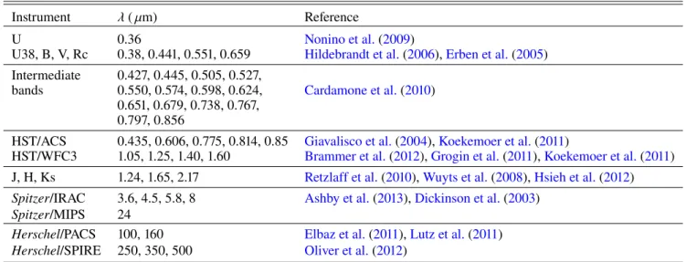
Table 1. Photometric coverage of the 7471 ZFOURGE galaxies used in this work.
Instrument λ ( µm) Reference
U 0.36 Nonino et al.(2009)
U38, B, V, Rc 0.38, 0.441, 0.551, 0.659 Hildebrandt et al.(2006),Erben et al.(2005) Intermediate 0.427, 0.445, 0.505, 0.527,
bands 0.550, 0.574, 0.598, 0.624, Cardamone et al.(2010) 0.651, 0.679, 0.738, 0.767,
0.797, 0.856
HST/ACS 0.435, 0.606, 0.775, 0.814, 0.85 Giavalisco et al.(2004),Koekemoer et al.(2011)
HST/WFC3 1.05, 1.25, 1.40, 1.60 Brammer et al.(2012),Grogin et al.(2011),Koekemoer et al.(2011) J, H, Ks 1.24, 1.65, 2.17 Retzlaff et al.(2010),Wuyts et al.(2008),Hsieh et al.(2012) Spitzer/IRAC 3.6, 4.5, 5.8, 8 Ashby et al.(2013),Dickinson et al.(2003)
Spitzer/MIPS 24
Herschel/PACS 100, 160 Elbaz et al.(2011),Lutz et al.(2011) Herschel/SPIRE 250, 350, 500 Oliver et al.(2012)
Notes. Only detections are considered in each band.
galaxies, such as stellar masses, instantaneous SFRs, dust attenu-ation, and SFH characteristics, taking into account panchromatic information from the SED. To perform the SED fitting on the ZFOURGE/GOODS-South sample, we rely on photometric red-shifts. For the sample used in this work, that is, considering the redshift and stellar mass selections, the precision of these redshifts is ∼3%.
In CIGALE, the assumed SFH can be handled in two differ-ent ways. The first is to model it using simple analytic functions such as exponential forms or delayed-τ SFH (see, e.g.,Ciesla et al. 2016,2017). The second is to provide more complex SFHs, such as those provided by semi-analytical models (SAM) and simulations (Boquien et al. 2014;Ciesla et al. 2015), an approach which we do not use in the present study.
3.2. Modeling and fitting the SEDs 3.2.1. Star formation history modeling
To identify galaxies that have undergone recent important varia-tions in their SFH from broadband SED fitting, we use the SFH implemented in CIGALE byCiesla et al.(2016) to model such a rapid decrease of the SFR:
SFR(t) ∝(t × exp(−t/τmain), when t ≤ ttrunc, rSFR× SFR(t= ttrunc), when t > ttrunc,
(1) where ttrunc is the time at which the star formation is instanta-neously affected, and rSFR is the ratio between SFR(t > ttrunc) and SFR(t= ttrunc):
rSFR=
SFR(t > ttrunc) SFR(ttrunc)
. (2)
Figure1shows an example of the truncated SFH (see Fig. 3 of Ciesla et al. 2016, to see the impact of each parameter on the shape of the SED).
This SFH has been presented and tested intensively inCiesla et al. (2016) where we showed that the agetrunc parameter (agetrunc = age − ttrunc) cannot be constrained from broadband SED fitting. However, the rSFR parameter is well-constrained
Fig. 1. Illustration of the SFH implemented in CIGALE. The purple dashed line represents a normal delayed-τ SFH with τmain= 10 Gyr,
without truncation or burst. The red solid line is the SFH showing a truncation modeling a rapid star-formation downfall and the green dashed-dotted line is a delayed-τ SFH on top of which we add a star formation burst.
especially in galaxies that were relatively active before the SFH variation. Comprised between 0 and 1, this parameter handles the strength of the rapid star-formation downfall in the SFH. Thus, we empirically showed inCiesla et al.(2016) that a star-forming galaxy with an output value of rSFRlower than 0.2–0.3 experi-enced a rapid decrease of its star formation activity in the last ∼500 Myr. However, when allowing rSFR values larger than 1, it is possible to add a recent burst in the star formation activ-ity of the galaxies modeling starburst galaxies. Thus, with this flexible SFH we are able to model a large variety of recent SFH (Ciesla et al. 2017).
3.2.2. SED fitting procedure
To model galaxy SEDs, we used the stellar population mod-els of Bruzual & Charlot (2003) and the attenuation law of Calzetti et al. (2000). The energy attenuated in UV-optical is re-emitted in the IR (mostly 8–1000 µm) through the models of
Fig. 2. Comparison between the true parameters of the mock SEDs and the results from the SED modeling with CIGALE. A parameter is well-constrained when there is a one-to-one relation between the two. Statistics on the ratio between the output and the input parameters are provided for the stellar mass and SFR: the first quartile of the ratio, the median, and the third quartile. The red dashed line in the rSFRpanel indicates the
threshold adopted in this study.
Table 2. Galaxy parameters used in the SED fitting procedures.
Parameter Value Delayed SFH age (Gyr) 0.5, 1, 2, 3, 4, 5, 6, 7, 8, 9, 10 τmain(Gyr) 0.1, 0.3, 0.5, 1, 2, 3, 4, 5, 6, 7, 8, 9, 10, 15, 20 Trunc. delayed-τ SFH age (Gyr) 0.5, 1, 2, 3, 4, 5, 6, 7, 8, 9, 10 τmain(Gyr) 0.3, 0.5, 1, 2, 3, 4, 5, 6, 7, 8, 9, 10, 15, 20 agetrunc(Myr) 100, 400
rSFR 0., 0.01, 0.02, 0.03, 0.04, 0.05, 0.1, 0.15, 0.2, 0.25, 0.3, 0.35, 0.4, 0.5, 0.6, 0.7, 0.8, 0.9, 1., 3., 6., 12. Dust attenuation E(B − V)∗ 0.01, 0.1, 0.2, 0.3, 0.4, 0.5, 0.6, 0.7, 0.8, 0.9, 1.0, 1.1, 1.2, 1.3 Dust template:Dale et al.(2014)
α 2.5
# of models 73,920
Dale et al.(2014). However, 71% of the galaxies are not detected by either Spitzer-MIPS or Herschel-PACS/SPIRE. To apply the same procedure with the same constraints to all galaxies, and to prevent the fit quality from being too strongly driven by the IR, we only fit the UV-to-NIR data of the galaxies, that is, up to Spitzer/IRAC4. We thus fix the shape of the dust emission since we do not study the dust properties of these galaxies.
To identify galaxies that have undergone a rapid decrease of their star formation activity, we perform the fit twice, once using a normal delayed-τ SFH and a second time using our truncated SFH. The input parameters used to perform the SED fitting are presented in Table 2. Even if we only consider star-forming galaxies, the defined parameter grids enable us to fit both active and passive galaxies in case of contamination by passive galaxies.
3.2.3. Constraints on the output parameters: mock analysis To identify the output parameters of the SED fitting procedure that we can trust and use in our study, that is, the parame-ters that are constrained with the photometric coverage available for the ZFOURGE sample, we perform a mock analysis. This procedure is thoroughly presented in several published studies (e.g., Giovannoli et al. 2011). Briefly, we first apply our SED
fitting procedure to the whole real catalog in order to retrieve the best fit SED for each individual source. Each best fit SED is then convolved with the set of filters available for the ZFOURGE sample and a noise is added to the mock flux, randomly chosen in a Gaussian distribution with a σ equal to the observed error. The original error of each filter is associated to the perturbed flux. We thus have a mock photometric catalog for which we know all the associated physical parameters from the output of the first run. A more detailed description on the mock tests implemented in CIGALE can be found inGiovannoli et al.(2011) andBoquien et al.(2012).
Then, we apply our SED modeling procedure a second time, but on the mock catalog and compare the output results to the true values of each parameter that we want to use in our study. These comparisons are shown in Fig. 2 for the stellar mass, SFR, and rSFR. As expected, given the good coverage of the rest-frame NIR, the stellar mass is well recovered and thus reliable. Although showing a larger dispersion for values between 0.1 and 10 M yr−1, the SFR is relatively well constrained with a relation close to the one-to-one line. The results of the mock analysis for rSFRshow that the parameter is, on average, always overesti-mated. We mention below that this does not affect our analysis or the identification of galaxies using this parameter since this overestimation simply makes our chosen threshold even more conservative (see Sect.4).
4. Identifying galaxies with a recent downfall of star formation
4.1. Selection criterion
We consider only galaxies defined as “star forming” from the UVJ diagram criterion of Whitaker et al. (2011) (see also Tomczak et al. 2014;Spitler et al. 2014;Straatman et al. 2014). Star formation histories of sources that have undergone a rapid decrease of their SFR (≤500 Myr) are not well fitted by models assuming a normal delayed-τ SFH, or an exponentially decreasing one, whereas the truncated SFH proposed manages to reproduce the UV-NIR SED (Ciesla et al. 2016, 2017). We thus expect that the χ2 obtained with a truncated SFH is significantly lower than those from the delayed-τ SFH for galaxies with a recent decrease of SFR as shown inCiesla et al. (2016). In Fig.3, we show the distribution of χ2obtained using both SFHs. However, the two SFHs have different numbers of degrees of freedom. To take this into account, we compute the Bayesian information criterion (BIC) for each SFH, using the definition:
Fig. 3. χ2 distribution obtained with the delayed-τ and the truncated
SFH for the whole sample and for the candidates (inset panel). The dotted line in the main panel indicates the cut made to eliminate the catastrophic fits.
BIC= χ2+ k × ln(n), (3)
with χ2the non-reduced χ2of the fit, k the number of degrees of freedom, and n the number of photometric bands fitted. We then calculate∆BIC the difference between BICdelayedand BICtrunc. If∆BIC is larger than two, then there is a significant difference between the two fits (Liddle 2004;Stanley et al. 2015), with the truncated SFH providing a better fit of the data than the delayed-τSFH. However, we impose a ∆BIC ≥ 10 to be conservative.
The second criterion is based on the value of rSFR. Indeed, from the study of Virgo cluster galaxies undergoing ram pressure stripping from the intra-cluster medium, we showed in Ciesla et al. (2016) that these galaxies, that underwent a rapid down-fall of SFR, have an rSFRof 0.3 and lower. Here, we consider that galaxies with rSFR≤ 0.2 are possible candidates, to be more conservative. Although calibrated from a study of galaxies well-known for undergoing a fast drop of their star formation, the value of 0.2 is mostly arbitrary. However, the goal of this study is not to select a statistically complete sample to derive prop-erties but rather to use broadband SED fitting to identify rapid phenomena. This threshold translates to a decrease of the SFR of at least 80% in the last few hundred million years according toCiesla et al.(2016) where we tested the sensitivity of the trun-cated SFH in terms of the strength of the star-formation decrease and its timescale. However, the overestimation of the true rSFR value revealed by the mock analysis (Fig.2) does not affect our criterion but rather goes toward strengthening it since an out-put value of 0.2 would be an overestimation of the true one. Finally, we impose a last criterion to reject galaxies with bad fits for both SFHs: we reject the 8% of galaxies with the largest χ2
trunc to remove galaxies with catastrophic fits. Quantitatively, we exclude galaxies with χ2trunc > 88.
From these three criteria, we identify galaxies as candidates if:
∆BIC ≥ 10 & rSFR≤ 0.2 & χ2trunc≤ 88. (4) The result of this selection is shown in Fig.4where we see that the large majority of the galaxies (98.5%) lie in the region where ∆BIC < 10 or rSFR > 0.2. We thus identify 102 sources satis-fying our criterion. The distribution of the χ2 obtained with the two SFHs is shown in the inset panel of Fig.3.
Fig. 4. rSFRoutput values as a function of∆BIC = BICdelayed− BICtrunc
for all the star-forming galaxies. The candidates sample is indicated by the gray filled region. For clarity, the x-axis is limited to [−20;75] but a few galaxies have higher∆BIC.
The best fits of six randomly selected sources (three normal and three candidate galaxies that have experienced a rapid down-fall of SFR) are presented in Fig.5. The three normal galaxies are displayed in the top panels where we see that the best fit SEDs are identical whether the normal delayed-τ or the trun-cated SFH is used. Their best fit SFHs are similar using either of the two SFHs, except for #562 where the truncated SFH prefers the contribution of a recent burst to reproduce the SED whereas the delayed-τ shows a younger age to reach the final SFR. The three other SEDs provide examples of fit results for three candidates. For these galaxies, the delayed-τ SFH does not manage to fit both the UV and the NIR or reproduce the Balmer break. Models built from a truncated SFH manage to reconcile the UV and NIR emission and provide good fits to the observed fluxes. For the three candidates, the best truncated SFH clearly shows a rapid and drastic decrease. For the delayed-τ SFH, in order to provide an equivalent final SFR, the age is shortened or the main peak of SFR is weakened.
4.2. The case study of three candidates
To understand the lower quality of delayed-τ SFH fits compared to the truncated SFH, we choose to study in detail the three can-didates, #20946, #20989, and #29927, whose SEDs and RGB images are shown in Figs.5and6, respectively. When running CIGALE, we are limited in the number of models to be fitted, and thus on the number of priors, due to computational reasons. The size of the prior grids, if reasonable, does not affect our results on the estimate of the physical parameters since we derive them through their probability distribution function (if the minimum and maximum values are well-chosen and the grid contains a significant number of values). However, it affects the value of the χ2 and thus can impact our selection criterion as the∆BIC is estimated using the χ2 of the fit for each model. Therefore, we check if∆BIC would be the same for these three galaxies if we used an increased grid of τ, age, and E(B-V), and if they would still fulfill the criterion. We run CIGALE using 100 values of τ (from 0.1 to 20 Gyr), of age (from 1 Myr to 13 Gyr), and of E(B-V) (from 0.01 to 1.5), successively. For each test, we provide in Table3the resulting χ2and∆BIC for both the truncated and normal delayed-τ SFHs. In each of these tests, the χ2 obtained with the truncated SFH is the same with variation of less than
Fig. 5. Best fits and best SFHs obtained for six example galaxies. The black points show the observations, the pink solid line the best fit obtained with the truncated SFH, and the gray dashed line the best fit obtained with the normal delayed-τ SFH. The six top panels show the SED and SFH of sources for which the two SFHs provide equivalent fit. The six bottom panels show examples of sources for which the delayed-τ SFH does not provide a satisfactory fit. The galaxies #20946, #20989, and #29927 have been selected as candidates. For #20989, the light blue curves in both the SED and SFH panels indicate the results obtained using a two-population SFH model (two exponentially decreasing SFHs).
ID20946
z
=0.61
Table 3. Robustness of the criterion against SED fitting priors.
I.D. nbands Main run Increased grid of τ Increased grid of age Increased grid of E(B-V) UV not fitted χ2 del χ 2 trunc χ2del χ 2 trunc χ2del χ 2 trunc χ2del χ 2 trunc χ2del χ 2 trunc
∆BIC ∆BIC ∆BIC ∆BIC ∆BIC
#20946 38 97.9 67.2 97.9 67.2 83.5 65.8 91.1 64.5 5.4 3.9 27.1 27.1 14.0 23.0 −2.2 #20989 36 107.0 65.2 107.0 63.2 83.5 63.0 80.3 62.6 10.8 9.9 38.2 40.2 16.9 14.1 −2.3 #29927 32 74.7 32.2 74.5 32.2 45.6 29.1 58.8 32.2 5.6 4.8 39.0 38.8 13.0 23.0 −2.3
5%. For the normal delayed-τ SFH, the χ2is improved up to 64% in the case of an increased age grid for #29927. However, despite these improvements in the normal delayed-τ χ2, these galaxies still fulfill the selection criterion with a ∆BIC larger than ten. Thus the difference we observe in the quality of the fits using the two SFHs is not due to the prior lists that we use for our main run. The UV should be the first spectral range to be impacted by recent variations in the SFH. Thus we test if fitting the SED of our three test galaxies without the UV rest-frame (<300 nm) fluxes would lead to a better agreement between the two SFHs. The runs are made with the increased range of age priors as we just showed that it improves the χ2 obtained with the normal delayed-τ SFH. The∆BIC obtained for these runs are negative with an absolute value lower than ten indicating that both SFHs provide an equivalent fit of the data (Table3). The UV is thus the key domain that the delayed-τ SFH struggles to reconcile with the optical-NIR part of the SED. However, as shown in Fig. 5, both the delayed-τ and truncated SFHs provide a good fit of the UV emission of #20989. Here, the discrepancy comes from the optical/NIR emission. One can then imagine that with the addition of an older population, that is considering two stellar populations, it would be possible to fit the NIR emission without the need for a recent fast decrease of the SFR. To test this pos-sibility, we fit the SED of #20989 using a double exponentially declining SFH, available in CIGALE, that allows two popula-tions combined through an extra free parameter. The χ2obtained with this SFH is 82.4 versus 65.2 for the truncated SFH, although the case with two exponentially declining SFHs has more free parameters. Thus a more complicated SFH is not preferred in this case. Interestingly, as shown in Fig. 5, the case with two exponentially declining SFHs favors a main stellar population with quasi-constant evolution plus a recent burst of star forma-tion followed by a rapid decline. The same test was applied to all the candidates and none of them were significantly better fit by a two-population SFH. Therefore, we conclude that the candidates underwent rapid and recent variations in their star for-mation, probed by the UV, something that is difficult to model using a smooth SFH.
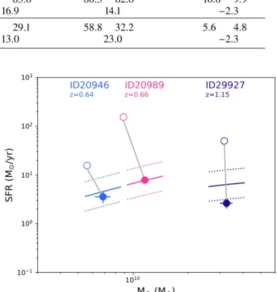
We show RGB color images of the three test candidates in Fig. 6. The sources #20946 (z= 0.61) and #20989 (z = 0.66) have a red disk and exhibit some UV emission as lanes. Their morphology suggests a merger scenario. In Fig. 7, we place them on the SFR-M∗plane along with the MS at their respective redshift. Both #20946 and #20989 lie above the MS prior to their decrease of SFR. Using the information provided by the SED fitting on the strength of the SFR decrease and knowing that it happened over a period of less than 500 Myr (the exact time is not constrained from broad-band SED fitting; see
Fig. 7. Positions of the three test candidates relative to the MS after (filled circles) and before (empty circles) the drastic decrease of star formation activity. The MS and its dispersion is indicated at the redshift of each candidate with a solid and dashed lines, respectively.
Ciesla et al. 2016andBoselli et al. 2016), we can recover their position on this plane before the decrease in SFR. They were thus previously even higher above the MS by a factor of 6.7 and 33.3 for #20946 and #20989, respectively, supporting the merger scenario. The question then remains of whether they will later remain on the MS or continue to fall and become passive. Fast decreases in SFR of these orders are consistent with the simulated SFH of mergers computed by Di Matteo et al. (2005). Interestingly, even the morphologies of #20946 and #20989 with a red disk and UV lane across the disk are consistent with the snapshots of their simulation. Since #20946 and #20989 are relatively low-mass galaxies, below 1.2 × 10¹⁰M
, we do not expect these mergers to have a strong dust enshrouded phase, allowing us to identify them from UV-to-NIR broadband SED modeling. The case of #29927 is slightly different as the galaxy is now below the MS. Previously it was indeed above, but, went down in a few hundred million years. This source is more massive with log M∗ = 10.51 and at higher redshift (z = 1.15). Its morphology (Fig. 6, right panel) shows a large red disk with a central bulge and a UV ring in the middle of the disk. There is also another source lying close to #29927 that could be an indication of possible interactions.
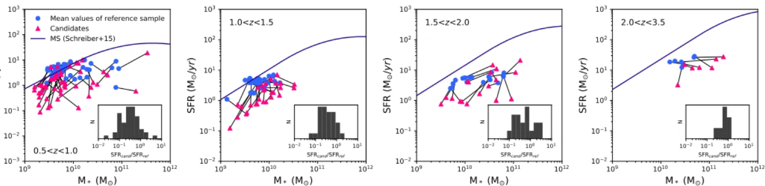
Fig. 8. Top panels:fitted galaxies placed on the MS diagram. The four panels show the MS in four redshift bins. Gray dots show the location of galaxies with good fits obtained with both SFH models and the pink triangles show the location of the galaxies selected as candidates for a possible recent drop of their star formation activity. Blue solid lines indicate the position of the MS at the mean redshift of the bin (Schreiber et al. 2015). Bottom panels:galaxies displayed on the UVJ diagram. Gray dots are the galaxies of the sample well fitted by both SFH models. Colored dots are the sources selected, color-coded according to the rSFR parameter. The black solid lines indicate the UVJ selection according toWhitaker et al.
(2011).
5. Physical properties of the candidate galaxies
To investigate the properties of these 102 sources, we place them on the MS diagram (Fig.8). They are mostly located in the lower part of the MS indicating a possible transition in their star for-mation activity. This is consistent with the hypothesis that these sources, selected using their SEDs, are undergoing a diminution of their SFR. Moreover, we observe that the candidates span a large range of stellar masses, from ∼109M to masses higher than 1011M
. Adding the information on the rSFR parameter allows us to see that the candidates located in the lower part of the MS still have some residual star formation showing that they are not totally quenched. Indeed, our criterion imposes a drastic diminution of about 80% of their star formation activ-ity in the last few hundred million years and not necessarily a total quenching. We then display the candidate sources on the UVJdiagram. We recall that our candidates are pre-selected to lie in the star-forming region of this diagram, which explains why none of them lie in the quiescent region. However, they are located in a region immediately below the passive region, close to the line separating the two zones, supporting the hypothesis that these galaxies are undergoing or have recently undergone a decrease in their star formation activity.
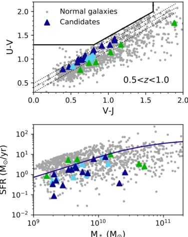
Recent studies have shown that galaxies displayed in color diagrams, such as UVJ or NUVrK, show a gradient of sSFR decreasing from the active region toward the passive region (Arnouts et al. 2013). We thus check if our selection is equivalent to an sSFR selection. To test this point, we separate our selected sample into three slices in the UVJ diagram, parallel to the line separating the active and passive region (Fig. 9, top panel). If they were selected from their sSFR value, we would expect these three slices to be recovered in the MS diagram. But, as shown in Fig.9(bottom panel), we recover no gradient of sSFR in the MS diagram; the galaxies are dispersed. This means that our
Fig. 9. UVJand MS diagrams for the first redshift bin (0.5 < z < 1.0). The normal galaxies are shown in gray, whereas the candidates (crosses) are separated into slices in the UVJ diagram. The slices used to separate the candidates are indicated with the black dotted lines.
Fig. 10. Comparison between the positions of the candidate sources (red triangles) and the mean values of their reference sample (blue circles) in the SFR–Mass diagram. The inset panels show the distribution of the ratio between the SFR of the candidate galaxies and their respective sample SFR.
criterion is not just a selection in sSFR and that we are able to select galaxies with SFHs that are different from the galaxies located in the same zone in the UVJ diagram. Indeed, as dis-cussed for the three test sources in Sect.4.2, the UV is a key domain to probe recent variations in the SFH and “normal” ana-lytical SFHs fail to reconcile the UV and NIR colors of our can-didates. But the UV is not used in the UVJ diagram explaining why we can find galaxies with identical UVJ colors but different SFHs.
5.1. Reference sample
The position of the candidate galaxies on the UVJ diagram shows that they are at the limit between the passive and the active galaxies regions, which could imply that these candidates may be undergoing a decrease in SFR. However, other galaxies are located in the same regions of the UVJ diagram and do not show any specific SED shape. To understand the difference between the candidates and the others, we define a reference sample. For each candidate, we select the galaxies that are located in the UVJ diagram at the same position and in the same redshift bin, within a circle defined as:
r h (V − J) − (V − J)q i2 +h (U − V) − (U − V)q i2 ≤ 0.2, (5) where (V − J) and (U − V) are the colors of the reference galax-ies and (V − J)q and (U − V)q those of the candidate. The 0.2 value is chosen arbitrarily after some tuning to ensure enough statistics to compute average properties of the reference sam-ple. Tests have been carried out to ensure that the results of this study do not depend on reasonable variation of the adopted radius.
5.2. Physical parameters
We compare the physical properties of the candidates to those of the reference sample. We average the properties of the galax-ies of each reference sample and compare the results to those of the corresponding candidate. In Fig.10, we place on the SFR-M∗ plane the mean values of the stellar masses and SFRs of the refer-ence sample corresponding to each candidate in the four redshift bins. The position of each reference sample, determined from its average properties, is systematically different from the position of the corresponding candidate galaxy. As expected, the SFR of the candidates is systematically lower than the average SFR of normal galaxies located in the same place on the UVJ diagram.
6. Morphology
With our method, we have adopted an empirical criterion to select galaxies that have recently undergone a drastic decrease of their SFR and have shown that their physical properties are different from those of galaxies with identical (U-V) and (V-J) colors. We now look at the morphology of the candidates. The morphological classification ofHuertas-Company et al. (2016) using deep machine learning is used to separate the candidates between spheroids (24 galaxies), pure disks (31 galaxies), disk plus spheroids (4 galaxies), irregular disks (20 galaxies), and mergers or irregular systems (12 galaxies).
We show in Fig.11the candidates in the MS and the UVJ plots, color coded as a function of their morphological clas-sification. There is no segregation of one particular type in a specific stellar mass range; spheroid candidates, as well as disks, are found at both low and high masses. However, at z > 2, the candidates are almost all spheroids or mergers, with only three disks out of 24 galaxies. Comparing the morphological types of the candidates with those of a reference sample is not straight-forward. Instead, we look at their effective radius, Recomputed by van der Wel et al.(2014). As shown in Fig. 12, the candi-dates and the galaxies of their reference samples cover the same range of effective radius (see inset panel of Fig.12). The median effective radii are 2.3 kpc and 2.5 kpc for the reference sample galaxies and the candidates, respectively. The first and third quar-tiles of both distributions are also consistent: 1.3 and 3.3 kpc for the reference sample galaxies and 1.8 and 3.4 kpc for the candi-dates. Therefore, we conclude that they have effective radii that are consistent with those of galaxies of similar stellar mass.
7. AGN activity
A possible source of rapid decrease in star formation could come from AGN activity as some simulations predict the AGN-driven outflows to be responsible for the downfall of star formation activity (e.g.,Baldry et al. 2004;Hopkins et al. 2006); although other results suggest that these outflows hardly affect the gas content of galaxies (Gabor & Bournaud 2014). Out of the 102 candidate galaxies, 5 are detected in X-ray (Cappelluti et al. 2016) and only 4 of them have an X-ray luminosity above 1042erg s−1: #1817, #3463, #10032, and #30250. The 4 sources with LX > 1042erg s−1 are massive with a stellar mass equal to or higher than 1.7 × 10¹⁰M .
Furthermore, we test whether some of these sources could host an enshrouded AGN emitting in IR. This can only be explored for sources detected in the MIR/FIR, and therefore we
Fig. 11. Main sequence (top row) and UVJ (bottom row) diagrams. The candidates have been color-coded according to their morphology classifi-cation as defined inHuertas-Company et al.(2016): in pink the spheroids, in blue the disks, in orange the disk+spheroids, and in green the irregular galaxies.
Fig. 12. Effective radius of galaxies with redshifts between 0.5 and 1 as a function of their stellar mass. Gray dots are all the galaxies in this red-shift range. Pink triangles are the candidates of this redred-shift range, and the blue circles are all the galaxies lying in the same part of the SFR-M∗
plane as the candidates, that is, the galaxies used to build the reference samples. The inset panel shows the distributions of Rein kpc for both
the candidates and the galaxies associated to the reference samples.
select the 47 candidate sources detected at MIPS 24 µm. Using the AGN emission modeling of the CIGALE code, we estimate for each source the need for an AGN template to fit the UV to IR SED. Out of the 47 sources, 23 have an output f racAGN parameter (contribution of the AGN to the total IR luminosity) below 10%. Based on the results of Ciesla et al. (2015), we can conclude that these sources do not likely host a strong IR AGN. Twenty-three sources have a trustable f racAGNparameter above 15%. However, among these 23 likely AGN galaxies, 18 of them have only one IR flux on which the decomposition can rely, which is not enough to provide a fiducial conclusion on the presence of an enshrouded AGN in these sources. Five candidates, however, have a high f racAGNbetween 30 and 50%: #1415, #10534, #15220, #17144, and #18949. Out of these five
sources, the SED of four of them indicates an unusually high IR 24 µm or 100 µm flux compared to the expected ones from the energy absorbed in UV-NIR (CIGALE performs energy balance), suggesting a possible blending problem in the IR photometry. This is confirmed by the fact that all four of these sources have a close companion. Only #18949 shows a clear sign of possible AGN contribution in MIR.
Out of the 102 candidates, only 5 of them show a sign of AGN activity either in X-ray or in IR. If it was to be interpreted in terms of duty cycle, considering that our method is sensitive to variations occurring less than 500 Myr prior to observation, this would imply an AGN duty cycle of 5%. Assuming that all the candidates went through an AGN-on phase, this would lead to an AGN visibility timescale of 25 Myr. However, given the poor statistics of AGN-detected candidates, we conclude that AGNs may not be the main cause for the recent decrease in star formation undergone by the candidate sources.
8. Probing recent movements relative to the main sequence
The epoch when the fast decrease in star formation occurred remains unconstrained from broadband photometry alone. How-ever, the SFR that the candidate galaxies experienced before the decrease is constrained by the rSFRparameter. This information allows us to locate the position of the galaxies with respect to the star formation MS prior to the decrease in SFR, that is, to deter-mine their past starburstiness (RSB, see Fig.13). The candidates fall into three categories, discussed below.
The first group is composed of sources that were lying in the starburst region, that is, above the MS, before undergoing the decrease in star formation activity and are now on the MS (Fig.14). These sources are thus post-starburst candidates. They have stellar masses lower than 2 × 10¹⁰M . Only one source is massive and is the most massive of the sample, #3463. Accord-ing to the morphological classification of Huertas-Company et al.(2016), 56% of the galaxies of this group are disks. This
Fig. 13. Starburstiness of the candidates before and after the strong decrease of their star formation activity as a function of their stellar mass. Filled circles indicate the position of the candidate at the moment they are observed, and the empty circles show the position of the can-didates prior to the SF decrease. Colors indicate different movements: from the starburst region to the MS (blue), from above to below the MS (purple), and from the MS to below the MS (red). The gray regions show the MS and its scatter.
is almost a factor three more than what is found for galaxies located in the same region of the SFR-M∗ (see Table 4). The remaining 44% are classified as irregular disks or systems ver-sus 57% found for “normal galaxies”. We notice the absence of spheroids in this candidate group when we expect about 23% of the “normal” galaxies to have this morphological type. With the data in hand, we cannot state whether or not these candi-dates are still in transition and thus just passing through the MS and will reach the passive region afterwards or if, after their star formation burst, they are back on the MS and will stay in this position for a given time. Going further in this analysis would require, at least, spectral information on Hα for instance, to compare different star formation indicators sensitive to different timescales.
The second group gathers candidates that were in the star-burst region and that are now below the MS (Fig. 15). These sources, which have stellar masses spanning a larger range, passed through the MS in a relatively short time which is of the order of several hundred million years. The distribution in terms of morphological types in this group is more balanced as we find 30% spheroid galaxies, 30% disks or disk+spheroids, and 40% irregular disks or system, versus 24%, 21%, and 55% for the reference galaxies, respectively (Table4).
The third group is composed of galaxies that were on the MS before and are now below it (Fig.16). These galaxies do not span a specific stellar mass range (Fig.13). The group is composed of a large fraction of galaxies classified as spheroids (36%) or as pure disks (39%). The median stellar mass of the galaxies clas-sified as spheroids is 2.3 × 10¹⁰M whereas the median mass of disks is 6.8 × 10⁹M
. This seems to indicate that the massive galaxies experienced a morphological transformation within the MS, prior to their rapid decrease in star formation activity. This morphological transformation may have been associated with the slow decrease associated to the bending of the MS (Schreiber et al. 2015). For the low-mass galaxies, the fact that they are classified as disks is an indication that they have some rota-tion, despite being well below the MS. The fraction of irregular
systems and disks is less important: 25% versus 44% and 40% for groups 1 and 2, respectively, and is almost a factor of two below the proportion of irregular galaxies in the reference sam-ple of this group (Table 4). We find galaxies with low stellar masses (≤1010M
) that departed the MS recently and now lie below it.
We find no significant behavior that could be different from one group to another based on the properties derived by our broad-band SED fitting procedure. We showed that the statisti-cal properties of our candidates point toward a recent decrease of star formation activity in this galaxies. However, we need spectroscopic data to validate the method and its use to quickly catch such galaxies in the act. Furthermore, to understand the different mechanisms that are affecting the candidate galax-ies of each group we need additional data in order to look for different star formation indicators, AGN activity, and gas content. Our method can be used to pinpoint galaxies with recent variations of SFH and to try to reconstruct these vari-ations, a first step to understanding the evolution of galaxies in the SFR-M∗ plane. Although this study focuses on galax-ies undergoing a decrease in star formation activity, it could also be used, in principle, to identify movements on the MS plane due to an increase in star formation. We find 233 can-didates with rSFR > 1 and ∆BIC ≥ 10 that will be explored in future work.
9. Conclusions
To probe and study phenomena that occur on very short timescales, we need large-number statistics to be able to catch them taking place. The goal of this work is to identify galaxies that have recently undergone a rapid (<500 Myr) and drastic downfall of their SFR (more than 80%) from broadband SED modeling, since large photometric samples can provide the statistics needed to pinpoint these objects. To this end, we choose to apply our method to the ZFOURGE sample to provide both statistics and large photometric coverage of the SED from UV to NIR.
– We fit the whole ZFOURGE sample using the CIGALE code with two different SFHs: one normal delayed-τ SFH and one truncated SFH, and usingBruzual & Charlot(2003) models. We show that a handful of sources are better fitted using the truncated SFH, that assumes a recent instantaneous break in the SFH, compared to the more commonly used delayed-τ SFH.
– Based on the results of Ciesla et al. (2016), we define a criterion based on the quality of the fits and the output strength of the decrease of star formation activity obtained from the SED modeling. From galaxies classified as “star forming” with the UVJ diagram, we select a sample of 102 candidates.
– We study three candidates in detail and show that the dif-ference of fit quality between the two SFHs is not due to the priors used for the SED modeling and that the nor-mal delayed-τ struggles to model consistently with the UV rest-frame and the optical-NIR emission.
– Placed on the MS diagram, these sources lie between the lower part of the MS and the passive galaxies region. In the UVJdiagram, they lie in a region in between the passive and active regions. This confirms the fact that these sources must be in transition.
– To understand their differences, we define for each candi-date a reference sample composed of galaxies lying in the
Fig. 14. Candidates that were lying in the starburst region before undergoing a fast decrease in star formation and that are now lying on the MS.
Table 4. Fractions of spheroids, disks, and irregular galaxies for candidate and reference galaxies, respectively.
Morphology Candidates Reference galaxies First group (postSB galaxies)
Spheroids 0% 23%
Disks 56% 20%
Irregulars 44% 57%
Second group (from above to below the MS) Spheroids 30% 24%
Disks 30% 21%
Irregulars 40% 55%
Third group (from the MS to below the MS) Spheroids 36% 25%
Disks 39% 29%
Irregulars 25% 46%
same region in the UVJ diagram and compare their physical properties.
– We compute the average properties of the reference samples associated to each candidate source. We show that despite their common location on the UVJ diagram, the candidate galaxies are displaced in the MS diagram compared to their reference sample. They have, on average, a lower SFR and an offset in stellar mass that seems to depend on the stellar mass of the candidate.
– There is no specific morphology attributed to the candidates. All types are found. Their effective radius is consistent with what is expected for galaxies of the same stellar masses. – Among the 102 candidates, 4 of them are detected in X-ray
with a luminosity larger than 1042erg s−1. Another source is classified as AGN from a UV-to-NIR SED fitting decom-position. This low number implies that AGN activity is not the main factor responsible for the fast decrease in the star formation activity of the candidates.
– Using the output of the SED fitting, we reconstruct the recent variation of SFR and show that the candidate galaxies are separated into three groups. The first one is composed of galaxies that were in the starburst regions and are now on the MS, which are thus post-starburst candidates. The sec-ond group is composed of galaxies that went from above to below the MS. The last group is composed of galaxies that were on the MS and are now below.
In this study, we provided and used a method to blindly identify galaxies undergoing a fast diminution of their star for-mation activity from their observed broadband SED. We showed that these galaxies have indeed physical properties that are different from the main population and characteristic of sources in transition. However, additional work is needed to confirm the variations in the recent SFH of these galaxies, especially using spectroscopy to look for strong Balmer absorption lines. Ancillary data are also needed to investigate the mechanisms at play and understand the possible role of mergers, AGN, and gas content.
Acknowledgements. L. C. thanks M. Boquien for useful discussions and B. Ladjelate for his help with Python. L. C. warmly thanks M. Boquien, Y. Roehlly and D. Burgarella for developing the new version of CIGALE on which the present work relies.
References
Abramson, L. E., Gladders, M. D., Dressler, A., et al. 2016,ApJ, 832, 7 Arnouts, S., Le Floc’h, E., Chevallard, J., et al. 2013,A&A, 558, A67 Ashby, M. L. N., Willner, S. P., Fazio, G. G., et al. 2013,ApJ, 769, 80 Baldry, I. K., Glazebrook, K., Brinkmann, J., et al. 2004,ApJ, 600, 681 Behroozi, P. S., Wechsler, R. H., & Conroy, C. 2013,ApJ, 770, 57 Boquien, M., Buat, V., Boselli, A., et al. 2012,A&A, 539, A145 Boquien, M., Buat, V., & Perret, V. 2014,A&A, 571, A72 Boselli, A., Roehlly, Y., Fossati, M., et al. 2016,A&A, 596, A11 Brammer, G. B., van Dokkum, P. G., Franx, M., et al. 2012,ApJS, 200, 13 Bruzual, G., & Charlot, S. 2003,MNRAS, 344, 1000
Buat, V., Heinis, S., Boquien, M., et al. 2014,A&A, 561, A39 Calzetti, D., Armus, L., Bohlin, R. C., et al. 2000,ApJ, 533, 682 Cappelluti, N., Comastri, A., Fontana, A., et al. 2016,ApJ, 823, 95
Cardamone, C. N., van Dokkum, P. G., Urry, C. M., et al. 2010,ApJS, 189, 270 Casey, C. M. 2012,MNRAS, 425, 3094
Ciesla, L., Charmandaris, V., Georgakakis, A., et al. 2015,A&A, 576, A10 Ciesla, L., Boselli, A., Elbaz, D., et al. 2016,A&A, 585, A43
Ciesla, L., Elbaz, D., & Fensch, J. 2017,A&A, 608, A41 da Cunha, E., Walter, F., Smail, I. R., et al. 2015,ApJ, 806, 110 Daddi, E., Dickinson, M., Morrison, G., et al. 2007,ApJ, 670, 156 Dale, D. A., Helou, G., Magdis, G. E., et al. 2014,ApJ, 784, 83 Dekel, A., & Burkert, A. 2014,MNRAS, 438, 1870
Di Matteo, T., Springel, V., & Hernquist, L. 2005,Nature, 433, 604
Dickinson, M., Giavalisco, M., & GOODS Team 2003, inThe Mass of Galaxies at Low and High Redshift, eds. R. Bender, & A. Renzini, 324
Draine, B. T., & Li, A. 2007,ApJ, 657, 810
Elbaz, D., Daddi, E., Le Borgne, D., et al. 2007,A&A, 468, 33 Elbaz, D., Dickinson, M., Hwang, H. S., et al. 2011,A&A, 533, A119
Elbaz, D., Leiton, R., Nagar, N., et al. 2018, A&A, in press, DOI: 10.1051/0004-6361/201732370
Erben, T., Schirmer, M., Dietrich, J. P., et al. 2005, Astron. Nachr., 326, 432
Fritz, J., Franceschini, A., & Hatziminaoglou, E. 2006,MNRAS, 366, 767 Gabor, J. M., & Bournaud, F. 2014,MNRAS, 441, 1615
Gavazzi, G., Consolandi, G., Dotti, M., et al. 2015,A&A, 580, A116
Giavalisco, M., Ferguson, H. C., Koekemoer, A. M., et al. 2004,ApJ, 600, L93 Giovannoli, E., Buat, V., Noll, S., Burgarella, D., & Magnelli, B. 2011,A&A,
525, A150
Gladders, M. D., Oemler, A., Dressler, A., et al. 2013,ApJ, 770, 64 Grogin, N. A., Kocevski, D. D., Faber, S. M., et al. 2011,ApJS, 197, 35 Guo, K., Zheng, X. Z., & Fu, H. 2013,ApJ, 778, 23
Heinis, S., Buat, V., Béthermin, M., et al. 2014,MNRAS, 437, 1268 Hildebrandt, H., Erben, T., Dietrich, J. P., et al. 2006,A&A, 452, 1121 Hopkins, P. F., Hernquist, L., Cox, T. J., et al. 2006,ApJS, 163, 1 Hsieh, B.-C., Wang, W.-H., Hsieh, C.-C., et al. 2012,ApJS, 203, 23
Huertas-Company, M., Bernardi, M., Pérez-González, P. G., et al. 2016, MNRAS, 462, 4495
Ilbert, O., Arnouts, S., Le Floc’h, E., et al. 2015,A&A, 579, A2
Koekemoer, A. M., Faber, S. M., Ferguson, H. C., et al. 2011,ApJS, 197, 36 Komatsu, E., Smith, K. M., Dunkley, J., et al. 2011,ApJS, 192, 18 Kriek, M., van Dokkum, P. G., Labbé, I., et al. 2009,ApJ, 700, 221
Lee, S.-K., Ferguson, H. C., Somerville, R. S., Wiklind, T., & Giavalisco, M. 2010,ApJ, 725, 1644
Liddle, A. R. 2004,MNRAS, 351, L49
Lutz, D., Poglitsch, A., Altieri, B., et al. 2011,A&A, 532, A90 Ma, J., Gonzalez, A. H., Spilker, J. S., et al. 2015,ApJ, 812, 88 Magdis, G. E., Daddi, E., Béthermin, M., et al. 2012,ApJ, 760, 6 Mancuso, C., Lapi, A., Shi, J., et al. 2016,ApJ, 833, 152 Maraston, C. 2005,MNRAS, 362, 799
Maraston, C., Pforr, J., Renzini, A., et al. 2010,MNRAS, 407, 830 Noeske, K. G., Weiner, B. J., Faber, S. M., et al. 2007,ApJ, 660, L43 Noll, S., Burgarella, D., Giovannoli, E., et al. 2009,A&A, 507, 1793 Nonino, M., Dickinson, M., Rosati, P., et al. 2009,ApJS, 183, 244
Oliver, S. J., Bock, J. et al. (HerMES Collaboration) 2012, MNRAS, 424, 1614
Pacifici, C., Kassin, S. A., Weiner, B., Charlot, S., & Gardner, J. P. 2013,ApJ, 762, L15
Pacifici, C., Kassin, S. A., Weiner, B. J., et al. 2016,ApJ, 832, 79 Pannella, M., Carilli, C. L., Daddi, E., et al. 2009,ApJ, 698, L116 Papovich, C., Dickinson, M., & Ferguson, H. C. 2001,ApJ, 559, 620 Pforr, J., Maraston, C., & Tonini, C. 2012,MNRAS, 422, 3285 Retzlaff, J., Rosati, P., Dickinson, M., et al. 2010,A&A, 511, A50 Rodighiero, G., Daddi, E., Baronchelli, I., et al. 2011,ApJ, 739, L40
Roehlly, Y., Burgarella, D., Buat, V., et al. 2014, inAstronomical Data Analysis Software and Systems XXIII, eds. N. Manset, & P. Forshay, ASP Conf. Ser., 485, 347
Salmi, F., Daddi, E., Elbaz, D., et al. 2012,ApJ, 754, L14 Salpeter, E. E. 1955,ApJ, 121, 161
Sargent, M. T., Daddi, E., Béthermin, M., et al. 2014,ApJ, 793, 19 Schreiber, C., Pannella, M., Elbaz, D., et al. 2015,A&A, 575, A74 Schreiber, C., Pannella, M., Leiton, R., et al. 2017,A&A, 599, A134 Scoville, N., Lee, N., Vanden Bout, P., et al. 2017,ApJ, 837, 150 Simha, V., Weinberg, D. H., Conroy, C., et al. 2014, ArXiv e-prints
[arXiv:1404.0402]
Speagle, J. S., Steinhardt, C. L., Capak, P. L., & Silverman, J. D. 2014,ApJS, 214, 15
Spitler, L. R., Straatman, C. M. S., Labbé, I., et al. 2014,ApJ, 787, L36 Stanley, F., Harrison, C. M., Alexander, D. M., et al. 2015,MNRAS, 453, 591 Straatman, C. M. S., Labbé, I., Spitler, L. R., et al. 2014,ApJ, 783, L14 Straatman, C. M. S., Spitler, L. R., Quadri, R. F., et al. 2016,ApJ, 830, 51 Tacchella, S., Dekel, A., Carollo, C. M., et al. 2016,MNRAS, 457, 2790 Tomczak, A. R., Quadri, R. F., Tran, K.-V. H., et al. 2014,ApJ, 783, 85 Tomczak, A. R., Quadri, R. F., Tran, K.-V. H., et al. 2016,ApJ, 817, 118 van der Wel, A., Franx, M., van Dokkum, P. G., et al. 2014,ApJ, 788, 28 Whitaker, K. E., Labbé, I., van Dokkum, P. G., et al. 2011,ApJ, 735, 86 Whitaker, K. E., Franx, M., Leja, J., et al. 2014,ApJ, 795, 104 Wuyts, S., Labbé, I., Förster Schreiber, N. M., et al. 2008,ApJ, 682, 985 Wuyts, S., Förster Schreiber, N. M., van der Wel, A., et al. 2011,ApJ, 742, 96